
Adaptive path planning for unknown environment monitoring
Abstract
The purpose of this paper is to offer a unique adaptive path planning framework to address a new challenge known as the Unknown environment Persistent Monitoring Problem (PMP). To identify the unknown events’ occurrence location and likelihood, an unmanned ground vehicle (UGV) equipped with a Light Detection and Ranging (LIDAR) and camera is used to record such events in agriculture land. A certain level of detecting capability must be the distinct monitoring priority in order to keep track of them to a certain distance. First, to formulate a model, we developed an event-oriented modelling strategy for unknown environment perception and the effect is enumerated by uncertainty, which takes into account the sensor’s detection capabilities, the detection interval, and monitoring weight. A mobile robot scheme utilizing LIDAR on integrative approach was created and experiments were carried out to solve the high equipment budget of Simultaneous Localization and Mapping (SLAM) for robotic systems. To map an unfamiliar location using the robotic operating system (ROS), the 3D visualization tool for Robot Operating System (RVIZ) was utilized, and GMapping software package was used for SLAM usage. The experimental results suggest that the mobile robot design pattern is viable to produce a high-precision map while lowering the cost of the mobile robot SLAM hardware. From a decision-making standpoint, we built a hybrid algorithm HSAStar (Hybrid SLAM & A Star) algorithm for path planning based on the event oriented modelling, allowing a UGV to continually monitor the perspectives of a path. The simulation results and analyses show that the proposed strategy is feasible and superior. The performance of the proposed hyb SLAM-A Star-APP method provides 34.95%, 27.38%, 33.21% and 29.68% lower execution time, 26.36%, 29.64% and 29.67% lower map duration compared with the existing methods, such as ACO-APF-APP, APFA-APP, GWO-APP and PSO-APP.
1.Introduction
Nowadays, obtaining information is becoming easier, with the complexity of accessing data being comparable to that of accessing a memory block. However, getting data from a sensor network is critical. Currently, data is collected through sensor networks. In the physical realm, data is collected for inspecting oil pipeline’s leakage, reviewing infrastructure for defects, researching water bodies to monitor the environment, and scanning risk events for relief operations. The limitation of fuel usage, as well as the length and distance of trip for data gathering, are notable issues in data gathering. As a result, path planning is an NP-hard task. The current state of the art systems take two approaches to solving this challenge. A myopic technique [10,56] is one approach, in which a set of sensing locations is determined and the system travels to the most promising one. While such solutions are computationally efficient, they fail to account for the travel distance constraint properly.
Various types of robots become popular for general, medical, industry and agriculture purposes. Unknown environment path planning for an autonomous exploration and simultaneous localization for agriculture robot got increased consideration [34]. Highest accurate environmental map is basis for bionic robot [28], autonomous vehicle [15], unmanned aerial vehicle [14] and Agricultural robot [24]. These robots achieve navigation, picking and placing things, surveying. The real challenge is the changing environment, variation in shape, illumination, occlusion, view point, etc. it is difficult to create maps for every real time scene. The absence of intelligent exploration of environment is cutoff the habit of robot expertise [48]. Consequently numerous researches originated to train robot, independently explore path planning for unknown environment, which permit the robot to develop dynamic map [26]. Optimal path plan generated by which is observed locally is combined with a partially created map [39,40,45,46,54]. The robot simultaneously predicts the map and updates the map to navigate along this trajectory [29]. Many researchers focused about the exploration of sensor’s position optimization. Full coverage observation of environment perception is achieved by frontier-based approach [32]. Frontier-based approach cannot guarantee the optimal trajectory plan because of its single stage greedy method [58]. By increasing the information gained through investigation, another method named multi step optimization used acquire optimal path [22]. Information gathering again based on monitoring the environment persistently. In many applications, maintaining the changing parameter is a crucial for managing uncertainty in environment path planning [2–4,12,17,19,20,23,35,37,41,43,44].
The evolution of robotics-based monitoring has ushered in a slew of new research opportunities. The fact that real devices have restricted amount of perceiving sources, like power, duration, or distance traveled, limits the number of observations which can be obtained is a major obstacle. Therefore, path planning need to planned extremely to maximize the time, energy, fuel. Path Planning plays vital primitive against autonomous agriculture robots that can find the shortest or otherwise optimal path between two points on the agriculture field or farm. Path planning is a route finding problem of effective outline to move the robot from the source to target. When the environment is newer than the path planning requirements, the map of the field requires the robot to be intelligent about its position. There are many robots available for real time scenario such as painting robots, cleaner robots, mining robots, lawn mower robots [43], Sowing robot 1 [37], Lumai-5 [2], Di-Wheel [44], and AgBot [17]. Path planning in agriculture are extend in various application. Two types of path planning proposed for agriculture robot: the first is point to point based path planning, the second is coverage based path planning [35]. In non-adaptive context, when the robots executed plan a path without accounting for noisy observations, the informative path planning (IPP) complexity is NP hard. The adaptive setup increases the difficulty by needing not only a strategy, but also a policy that adapts to the observations the agent receives. We further expand the problem by explicitly introducing different sensing modalities and taking into account the impact of both sensing and moving on the energy budget [4].
Autonomous robots are collectively working to gain worthy data about our regions. In the older days, rapid technological advances have unlocked unique stages of autonomy and decision-making of their perception just in case of flexible and cost effective tool [20]. Strategies are sapping conventional data collecting procedures using fixed sensors, conventional sampling, or manned platforms that are steered in aquatic applications, this can be inconvenient, costly, and even deadly [23].
Rational devices focus a challenge that is limited size of sensing resources, for example distance, session, energy, which restricts the quantity of factors which can be gathered. Hence, path must be well planned, enlarge the information gather about the unknown environment, whereas fulfilling the set of budget constrain. This IPP issue, which is the focus of current research, despite ongoing improvements in this field, most of the robot acquired data in passive manner only. IPP using coverage-based path planning are usually restricted to a few platforms or application domains. Intelligent vehicles are an intelligent agent which consist of environment perception & modeling, localization with mapping, path planning with decision-making and motion control.
Mostly others have spent their effort by comparing algorithms in order to determine which can provide the most precise map. Every method has such a set of conditions that can be tailored to the turtle’s work atmosphere. Factors like robot rapidity, plotting apprise interval can affect not only how long it takes but also how accurate the map is. As a result, it is vital to understand how different algorithm settings modify map characteristic, which is the focus of this research, particularly when robots are operating in unfamiliar environments especially when robots are working in unknown environment.
Formerly, fuzzy logic and neural networks were used to produce a variety of control programmers, system identification techniques, and active disturbance rejection platforms. While neural networks have complex neuron controllers, designing a fuzzy logic controller requires expert knowledge. Although the Negative-Imaginary (NI) theory is applicable to robust vibration control issues for adaptable structures with high-resonant dynamics, most approaches based on this theory have not addressed the challenge of high-precision trajectory monitoring for quad rotor structures in environments that vary.
Machine learning strategies are widely used in autonomous robots in recent years. These robots are equipped with adaptive learning capabilities based on acquired knowledge. An essential subfield of machine learning is reinforcement learning (RL), which continually updates an agent’s activation policies in response to feedback dependent on the situation by trial-and-error. The availability of training samples has increased due to the advancement of simulation technologies and the accumulation of measurement data. Due to its strong ability to learn in challenging contexts, reinforcement learning is shown feasible outcomes in the navigation of mobile robot. The designing of track planning approach polished, then these algorithms parameter improved by valuable facts. Early research also employed ML to increase the environment awareness, which is huge, dynamic, or partially unstructured.
Also, manually tuning complex control loop requires more time to controller experts. Additionally, single-objective criteria like small chasing fault, short mounting time and minimum overshoot are satisfied via manual parameter tuning and optimization. Therefore, intelligent embedding method is presented to deal these issues. The global optimization strategies for parameter tuning contain genetic algorithm, ant colony optimization, particle swarm optimization, reinforcement learning etc. Due to comprehensive onboard implementation, Machine Learning strategies allow automatic adaptation to environment. But define the performance of potential tuning parameter solutions and gather a big size of information through relevant real-world domain, its evaluation framework necessitates a significant amount of time. There are other sources of uncertainty that could contribute to the multiple disruptions in performance evaluation (sensor noise or manufacturing tolerances). Significant research theme at robotics is the higher-performance route track of unmanned aerial vehicle by effect of aging as well as environment. Its advantages contains a broad spectrum of application in civilian and military domain, like aircraft review, following, implementation of law, wildlife observing. If robust systems of control are not designed to withstand the impacts of external commands and disturbances, this sort of uncertainty results in poor performance or instability in the system. Despite the fact that numerous path-following control strategies have been investigated to mitigate the impact of the additional wind component, there is a high reliance on wind knowledge and a standard PID monitoring controller architecture with no active anti-disturbance features capacity compared to other tuning models.
As already indicated, the majority of existing path planning approaches in use mainly relies on a static global map. When the map contains vibrant restrictions, its state requires to be recognized. These algorithms may act badly with unknown static with dynamic obstacles and frequently get orientation track instead of velocity facility, so extra sensors or tracking techniques must be used, which complicates navigation along computation for the mobile robot.
This is the reason behind the motivation of this research. To overcome the shortage of autonomous vehicle especially for unknown environment depends on accurate map to achieve the effective path planning and improve optimization for agriculture phenotype robot and enhance the persistent monitoring based on region of interest. The key contribution from our side work is a HSAStar mapping approach for point cloud data is utilized to calculate the various spatial arrangements for unknown environment. Then save them in the map to promote persistent monitoring. Hybrid SLAM & A Star algorithm for path planning is convenient to activate with the parameters for tuning. It proves a greater convergence, lesser computation time, and better proficiency to determine global optimum. Obviously, its recall ability is more effectual than learning algorithms, because every star can able to concurrently signify own preceding better place and neighborhood better.
1.1.Literature survey
Path planning algorithm for environmental exploration has two kinds. The first was myopic, which selects one step at a time as its next move. The study does not address the lack of anticipation mechanisms, which could be tricky in route planning and decision-making. The second technique was based on a partially observable Markov model that consigns a reward to each allowed action sequence. The computational complexity in non-myopic techniques was high. [33]. Using the evidential gird framework, Mouhagir et al. presented trajectory planning for autonomous vehicles in an uncertain scenario. The presented study models the integration of environmental uncertainty with an evidentiary grid, demonstrating great performance in avoiding barriers. The robotized vehicle was not implemented [8].The authors presented a novel acquisition technique for informative path planning, which was created for the purpose of detecting anomalies in exploration missions. The proposed algorithm was tested on synthetic test functions in the real world. The authors propose that a three-dimensional (3D) search space be added to the two-dimensional (2D) path parameterized technique. For complex time dependency of the environment, a covariance function was proposed, which encodes particular spatiotemporal surveillance.
The research was employed to detect anomalous quantities in a certain area of chemical substance, contaminants, or radioactive substances, as well as need to re-create a landscape with undefined terrain for large-scale architecture [38]. The research introduced an innovative deterrent deliberate IPP calculation that was useful for UAV target search problems. To generate the ideal, limited skyline 3D polynomial route in a major impediment climate, the organizer strikes a balance between inclusion, obstruction aversion, target re-perception, height subordinate sensor execution, flight time, and FoV. The presented layered improvement strategy was effective against fraudulent identifications since it was combined with a good investigative abuse mechanism.
In terms of search efficacy, the presented organizer outperforms the non-versatile IPP organizer, the inclusion organizer, and the arbitrary examining organizer [21]. The calculation took into account a wide sort of climate complications and barrier densities. Despite multiple bogus human recognitions by the sensor, it successfully tracked down all of the persons a meaningful SAR reform on the ground, demonstrating the vigor provided by the layered advancement technique. The organizer’s primary flaw was that it assumes a constant and predictable climate. Furthermore, for target inhabitance, a non-transient field was expected.
Researchers employed an informative continuous space path planning algorithm, evaluated the measured data online, and reasoned near the suitable measurement point. The presented method permits the robot to replan adaptively sampling in position, so that focus on a specific feature of interest. That technology was used in UAV-based gas distribution mapping, ground ice mapping with a rover, and monitoring with a catamaran-type ASV [7]. Bricher and teams introduced Receding Harizon planner for a known or unknown environment, the suggested planning approach finds noble paths for inspecting an a priori known surface. Additional effort might be devoted to developing plans for numerous robotic platforms, such as large-scale trials, fixed-wing Drones or automated machines [36].
SankalpArora and Sanjiban invented Partially Observable Markov Decision Processes (POMDP) were a simple way to simulate sequential decision making in uncertain situations. MDP-POMDP solvers accomplish multi-resolution gen collection task poorly at the budgeted and do not take advantage of UAV agility, rendering them inappropriate for such applications [5]. Olov Andersson presented a combining optimum and Actual planning of physically feasible pathways in tough situations with dynamic barriers by receding-horizon control with space-time multi-resolution lattices. Researchers have shown the context in action via handling complex indoor 3D quad copter situations of navigation that need planning ahead of time. Waiting for other people and quad copters, as well as taking diversions around them [30]. Qing and team explores path searching, it records all equidistant shortest paths and chooses the best path among numerous equidistant paths based on the turn time, resulting in the path with the shortest distance and time [47].
Yu Feng, Shaoshan Liu and Yuhao Zhu proposed spatially encoding the sequence’s key for point-cloud, which was usually the middle one. The K-spatial frame’s encoding discoveries utilized to temporal encode the remaining point clouds, which refer to as expected point clouds (P-frames) (P-frames). Autonomous machines was able to connect more with each other and cloud using well organized point cloud compression, entering a new period of distributive and cloud robotics. The study by Rekleitis et al. [42] presents a spatio-temporal technique for compressing Light Detection and Ranging (LIDAR) point clouds. For a variety of reasons, IoannisRekleitis and Jean-Luc Bedwani have chosen a LIDAR as the primary sensing mode: for example, the mobile device has vastly limited ground consent. LIDAR sensor can provide range data that can be used to construct landscape models with a resolution of 1–2 cm. Most stereo vision systems would struggle to achieve such precision over the whole measuring range. Such precision was also critical for the mission’s scientific return, which includes detecting rock formations.
Furthermore, without the need for extra processing, LIDAR sensors deliver precise 3D geometric information in the shape of a 3D point cloud [6]. The planning of a receding horizon trajectory based on optimization approach [18] introduced by Kristoffer Bergman for nonlinear dynamics functioning in a congested and unstructured environment. To handle the 3D Path Planning problem in a dynamic setting, Utkarsh Goel and Shubham developed on the Glow-worm Swarm Optimization (GSO) algorithm. The application of Swarm based Intelligence allowed for more rapidly convergence, which increases the efficiency of path planning. Based on findings obtained when completing the model, the feasibility of Path planning for UAVs in a 3D Dynamic Environment was extrapolated utilizing the presented approach [27].
In Chen et al. [11], path planning and obstacle avoidance of USV based on enhanced ant colony optimization-artificial potential field (ACO-APF) hybrid algorithm with adaptive early warning was described. The technique described was based on a grid map for USV local and global path planning in dynamic situations. The ACO algorithm sought a globally optimal path from start to endpoint for USV in a grid environment, whereas the APF method avoided unexpected obstructions during USV navigation. It delivers greater accuracy while using a smaller map size.
Cao et al. [9] showed 3D Snake-Like Robot Motion Direction Control and Adaptive Path Following. The adaptive path-following was based on the line-of-sight guiding law and was used in conjunction with the direction control approach to steer the robot forward and along desired courses. The findings show the effectiveness of the given 3D model and control approaches. It outperformed the standard and widely used path-following model. It has a longer map duration but a shorter patch length.
Abed et al. [1] demonstrated an online optimisation application for path planning in unknown environments. Grey Wolf Optimisation (GWO) variants MGWO1 and MGWO2 were proposed for online route planning to help the mobile robot reach the target using the shortest path and avoid obstacles in unexpected surroundings. To avoid abrupt curves, a cost function was created by combining the path smoothing parameter with an integrated distance function. The findings showed that the provided GWO, MGWO1, and MGWO2 algorithms were capable of successfully ignoring barriers in a local minima condition. It has a faster execution time and a smaller map size.
In Tran et al. [52], adaptive trajectory tracking for quad rotor systems in uncertain wind settings using particle swarm optimization-based strictly negative imaginary controllers was described. The notion of adaptive strictly negative imaginary (SNI) controllers is introduced by particle swarm optimization. The provided adaptive control methods reduce a certain performance index, showing the control design’s goal. It gives greater precision while having a shorter patch length.
From the literature, the research gaps are identified by the authors and listed here, a variety of robotic platforms, such as large-scale test scenarios, UAVs, or robot arms have to develop to maximize the performance of autonomous vehicle [36]. First, the presented receding horizon planner has been designed to work in dynamic contexts. The presented approach scaled to bigger areas in the future, and the mapping model extended to capture temporal dynamics. It allows the use of previously gathered data as a baseline in long-term monitoring missions to increase real-time performance. Second, the receding horizon planner has been designed to work in dynamic contexts. Another extension is to use principles from fast MPC to increase real-time performance [6]. Third, to improve robustness, obstacle motion uncertainty must explicitly be included [30]. Fourth, the path planning process can be combined with Deep Learning or SLAM to assist UAVs to create a real-time map of the environment [18].
This work uses the Gmapping SLAM method using a mono laser sensor for mapping and localization. Furthermore, the Data-matching method is employed to support a more exact map based state position estimation. A portable system is a system that is portable in terms of hardware intended to run an algorithm. The research’s scope is to create a rough map of the area using portable devices. In the shortest amount of time and for the least amount of money, a handheld system is created. Pre-mapping is the term for this procedure. Premapping provides a solution to the chicken-and-egg conundrum other difficult issues in SLAM algorithms [31]. In this investigation, a single laser is used to maintain the solution. Sensor that uses the Gmapping technique only using a laser sensor measures as a data source for localization and mapping. In varied settings, just laser pixel intensities, IMU sensor and wheel encoder were employed for identification and mapping as data for pre-mapping. Pre-mapping is a low-cost solution to problems with autonomous exploration and navigation.
1.2.Contribution
The goal of this research is to propose a realistic solution to the problem of continuous monitoring in an unknown environment using Unmanned Ground Vehicles (UGV). This method is used to detect the Indian agriculture fields which does not have proper road. It is not having defined road signs and objects like vehicle, pedestrian. But these roads may have uncertainties like varieties of plants, trees, ridges, size of the path, etc. So, extracting or identifying such type of path helps to navigate the robots in the form field. It help to extent for many type of applications related to agriculture purpose. The subject was investigated in terms of collect the data about the environment, interpret the data for modelling and path planning, finally control the vehicle to follow path. The presented method contains the following five contributions when compared to related work and existing technology.
(1) A novel problem for persistent monitoring on the unknown environment like agriculture field, employing UGVs, which is called the Persistent Monitoring Problem (PMP). The development of “region” is designed with a given analysis along the path to improve the monitoring effect.
(2) For addressing unknown environment path planning, HSAStar algorithm is suggested for path planning and a modelling. To the best of author’s knowledge, UGV embed with HSAStar algorithm is the first solution to the problem of continuous monitoring and path planning in an unknown environment. In this approach, the problem modelling approach is an event-oriented strategy that formulates the PMP based on the nature of the occurrences and the UGV’s genuine ability to identify. Based on model’s features, a HSAStar algorithm for path planning approach which is suitable for the PMP is designed from a decision-making position.
(3) As a consequence, the suggested method modifies the motion parameters and reduces the velocity prior to the start of the experiment to avoid the motion route from diverging from the planned path due to the too high velocity at the entrance and exit places.
(4) The randomly produced tracking path is pretty simple, and the tracking experiment shows a considerable gap among the tracking path and obstructions. It keeps variations from the planned course from occurring due to inadequate security barrier.
(5) The tracking coordinate points are widely dispersed throughout the tracking line, and the mobile robot navigates them in a sequential manner. It enables the robot’s excellent accuracy in tracking during the tracking procedure.
The remaining sections of this article are organized as follows: Section 2 describes the problem formulation for SLAM based persistent monitoring problem for agriculture environment. In Section 3, the PMP’s decision variable in SLAM based path planning is proposed. System design for persistent monitoring enabled robot using Hyb-SLAM-AStar algorithm is discussed in Section 4. In Section 5, experimental results are proved, Section 6 portrays the discussion and Section 7 presents the conclusion and future work.
2.Problem statement
For a robot travelling across a landscape, our design stresses data-gathering strategies. The goal is to gather as much environmental data as possible while remaining within power, spell restrictions and distance costs are examples of resource constraints. This problem is properly called as path planning for efficient data gathering and is defined as follows. This section explains how to formulate the Persistent Monitoring Problem it is frequently used to represent persistent surveillance problems by dividing the space into separate cells with a measurement [16,57] are concerned with the effects of monitoring. We make use of the graph to develop the discrete model, use theory as a simplification technique of the actual path formation, which is made up of perspectives as well as the edges. UGV has a monitoring influence on the viewpoints. Sensor detection ability was used to calculate the value based on the PMP formulation form is supplied on the above. The purpose of this paper is to show how a UGV may cover a large unknown a large region in a short period of time while detecting a large number of events. We’ve seen events that we’re concerned about out of nowhere in an unknown setting. The likelihood of their occurrence as well as the regions of their occurrence are unclear. Although the exact time of an event’s commencement is unknown, its length can be calculated statistically [55]. If the UGV accurately detects a continuing event, it signifies the UGV has fruitfully record the event’s incidence in an unknown environment [13]. To put it another way, if the incident lasts longer than the spell between two exact UGV monitoring excursions on same point, it can be located at any time. Finding UGV trajectories with a specific coverage limit while they are moving in order to maximize a scrutinizing norms related to the observing effect. Priorities, based on the likelihood of an event occurring and its location are a mystery.
The PMP task environment model is abstracted into a node represents connected
In this, the uncertainty is a problem reduced by assuming the robot, the relative pose of teammate ca be derived from relative distance ρ (presented via laser), the angle
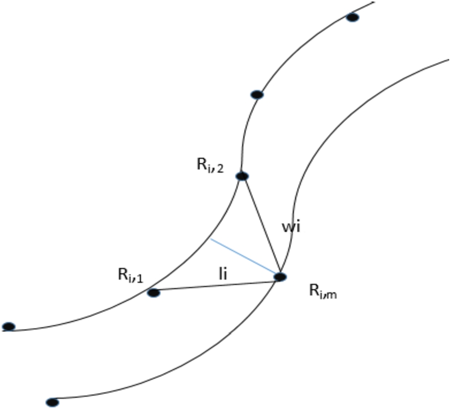
Step 1: Path quantization
(1) Path Estimate: The largest separation between two points
(2) Path Segmentation: The curve segmentation point is defined as the farthest point
(3) Path Revision: Insert entire recent data from previous stages to R, W for those paths and
Fig. 1.
Discrete process of path.
Step 2: Long Path Segment
Any road
Step 3: Creation of Grid Representation
Entire intersections created through preceding phases are referred to as views and are denoted by the letters
2.1.Problem definition and assumptions
Likewise the above mentioned task of warehouse, the uncertainty issue is solved by modifying the motion parameter and lowering velocity prior to the start of the study in order to avoid the motion route from diverging from the planned path due to the too high velocity at the entrance and exit points. The robot’s initial position and target are pre-set, the robot recognizes the global map outline (walls of warehouse), i.e, the problems in map are entirely unidentified. The aim of the robot is to reach the destination while keeping a safe distance from the obstacles. The robot can reach the destination at any velocity and does not need to stop.
In addition to the global map’s layout, robot’s many sensors provide all the information it can (gyroscope, lidar, encoder). These sensors can be used to gather the data needed by the proposed method at each time step. Make given assumption regarding navigation issue.
Assumption 1.
The robots place, alignment and velocity at the global map identified in every time step.
Assumption 2.
The target place in the global map identified in every time step.
Assumption 3.
The closest obstacle distance in each circle direction is identified at every time step. These data structure is exhibited as
The robot is differentially propelled and considers itself to be moving forward along a rotating axis. Equation (4) depicts the robot’s kinematics theory.
3.Method proposed for path planning under an unknown environmental using hybrid Simultaneous Localization and Mapping (SLAM) with A Star Algorithm
3.1.Simultaneous Localization and Mapping (SLAM):
SLAM allows the rapid creation of navigable outlines that converts as navigable spaces and maps. This is impractical to use manual methods for mapping indoor environments, because of complexity and size of indoor space. Traditional SLAM has been used primarily in the field of robot navigation, requiring high level of output precision in order to be useful for robot movement maps. This has prompted research on more effective and quick sensors, measurement techniques, and measurement data post-processing. However, every improvement in accuracy has been accompanied by an increase in processing or equipment costs.
The Robot Operating System (ROS) platform, which is existing in Ubuntu, may be used to do SLAM, It is among the approaches for mapping robots on the move. GMapping is used as the algorithm for this study. The responsibilities of cartography, positioning, target tracking tasks, overlapping hitches. The difficulty of constructing a map while simultaneously localizing a robot within that map is known as SLAM. Both tasks can’t be decoupled and solved separately. Localization requires a good map, whereas building a map necessitates an accurate pose approximation. To improve the pose estimation, the goal of effective localize is to guide the robot to specific locations on the grid. Exploration approaches, on the other hand, presume precise posture knowledge and concentration on efficiently directing the vehicle across the surroundings in order to develop a map.
Fig. 2.
Key component process of the robot.
Solutions to the SLAM problem are sometimes known as integrated techniques. The key component process of the robot using SLAM algorithm is shown in Fig. 2. The Rao-Blackwell zed Particle Filter (RBPF) is utilized by G Mapping to collect data laser sensors and other sources. Make a 2D grid map with a robot stance [50]. In essence, the fundamental issues in map learning are listed as what place to steer a robot on a mission of self-exploration, how to handle noise in posture estimate and observations, and how to manage with ambiguity and how to interpret it data from sensors, how to effectively manage a team of mobile robots and variations in the echo system over time [59]. The mapping flow procedure is depicted in Fig. 3.
Fig. 3.
Environment mapping flow process.
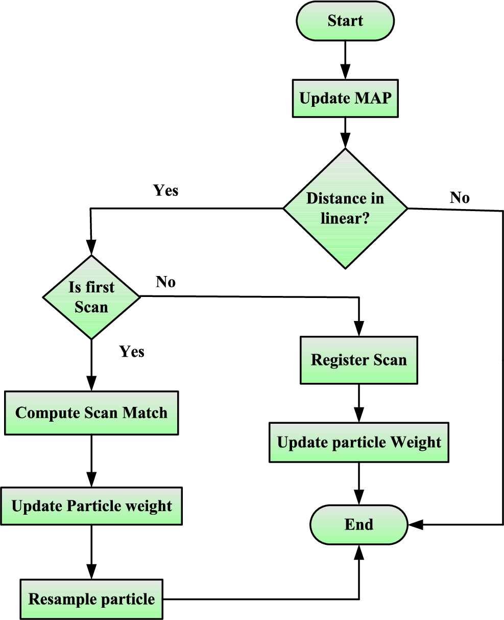
There are a number of advantages to using GMapping as the primary HSAStar technique in this work. For starters, it’s an open source, algorithm which is ready to use, that’s part of the Robot Operating System (ROS). Second, it is deep rooted and has a proven track record, as evidenced by recent publications such as [31]. Finally, because the approach is a solo threaded technique in which each element is calculated separately, it lends itself nicely to parallelization. This is a good situation named at parallelization because there is no want to transfer data to particles. Whenever the robot acquires a fresh laser shot, the program executes steps outlined in the flowchart in Fig. 3. The vehicle alters the posture of the whole examined particle throughout execution based on odometry estimate using its motion model. The first scan is immediately recorded in the map when it is received. After that, only if the robot’s linear or angular distance traversed exceeds specific thresholds is registration performed. After that, data acquisition match is performed, which corrects pose estimation in each particle’s map. As a result, the particle tree’s weights have been adjusted, as has the effective sample size
For posture estimation and map generation, this study uses the data-matching approach then the grid representation using Gmapping algorithm. As illustrated in (4), HSAStar algorithms are frequently built on a common filter using probabilistic Bayes, with specific data being used to assess the density of an unknown probability density. The Bayes Filter, also known as Recursive Bayesian Estimation, is the foundation of several probabilistic techniques in robotics. A state, such as a robot stance, is represented by a Probability Density Function, or pdf, in Probabilistic Robotics. Another term is belief, which refers to the robot’s internal knowledge, rather than ours, from its perspective. The Bayes Filter is a general method for iteratively estimating a state’s pdf using a Mathematical Process Model and Measurements.
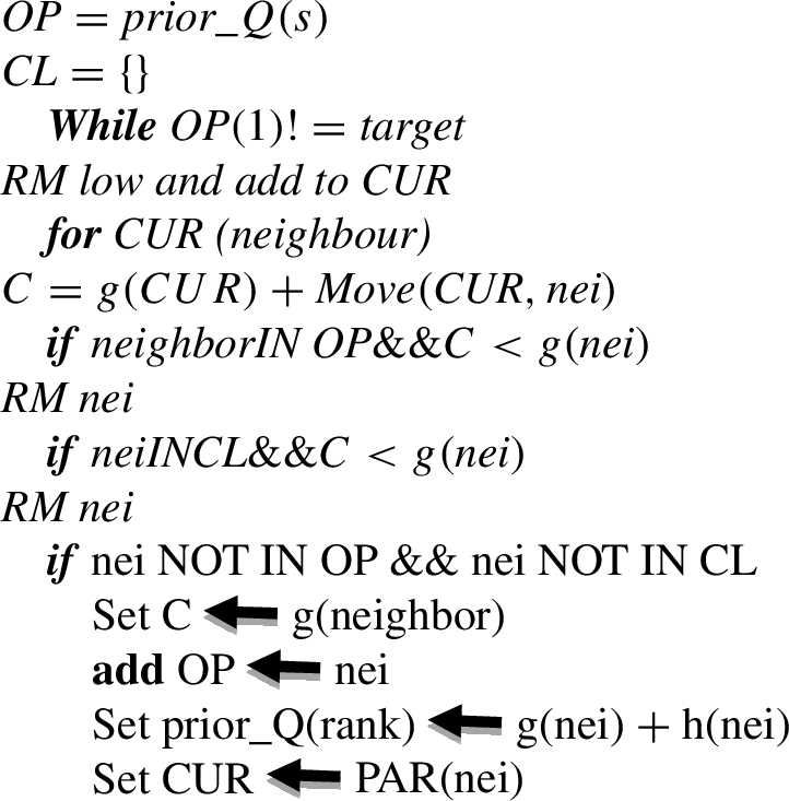
3.2.A Star algorithm for point cloud data
A Star is equivalent to Greedy Better in that it uses a heuristic to direct itself. In the simplest instance, it’s as speedy as Greedy Best-First-Search. In standard
Algorithm 1
AStar (point cloud data)
3.3.Grid mapping
The Gmapping method is employed as a HSAStar approach in this investigation. It employs the particle filter to acquire lattice representation after laser range sensor data. Using laser scan measurement data
Algorithm 2
Hyb SLAM A Star (point cloud data)
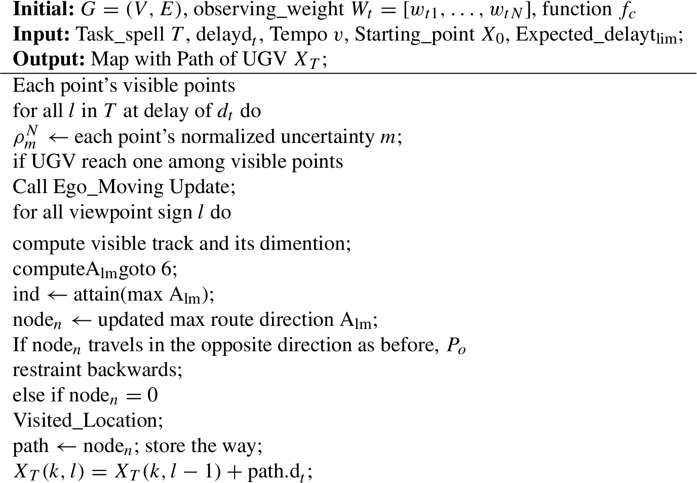
ego_Moving Update: A ego_Moving update adjustment function of pc is set based on the discussion of the reward coefficient pc to increase continuous observation performance. Restraint backwards: The go_back of the UGV will unavoidably occur in path planning because of the heuristic technique’s randomness and the change in payout. When the go_back occurs, however, it is difficult to assess if this decision is sensible or not. As a result, the suggested approach allows the UGV to return to its new path. Visited_Location: UGV is said to be in a loop closure once the path budget exceeds payment or when the budget of various positions are equal. To boost monitoring efficiency, when a loop closure occurs, the viewpoint by the greatest payment of altogether neighboring viewpoints at present prespective is picked as the goal points for the following second.
4.System design
Before we can do SLAM research, we need to put up a mobile robot experimental platform. The main control uses ESP8266 Node MCU microcontroller and Raspberry Pi 4 as a Microprocessor to achieve the benefits of low cost, modularity, flexibility, and expandability of mobile robots. To complete the design of the entire hardware system, the robot bottom stage control panel employs the raspberry driver board for Image processing and ESP8266 Node MCU board to connect to a station point to transmit the data from our ESP32 Camera Module and VL53L1X Lidar Sensor and for the robot’s locomotion we use Gear Micro DC Encoder Motor which is connected to a Node MCU Motor Shield and a Step-Down Transformer to regulate the voltage supply [60].
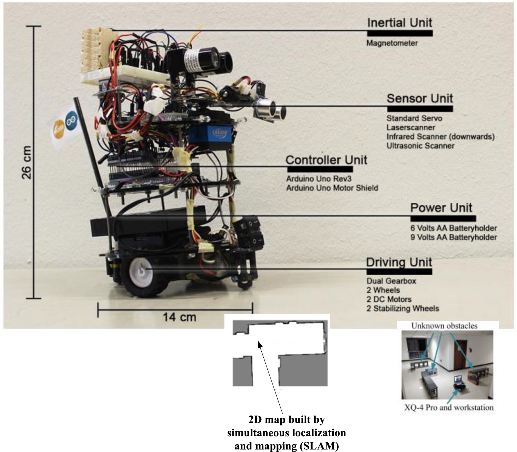
Fig. 4.
Ground vehicle frame design.
4.1.Body of a mobile robot platform
Mobile robot’s structure made up of 2 layer of acrylic plate. It measures 35 centimeters by 20 centimeters by 15 centimeters and weighs about 3 kg. It may make a range of sensors and devices to fulfill the experiment’s necessities. The authentic thing of a ground vehicle is depicted in Fig. 4. The experimentation is done on unknown environmental along the obstacles of static or dynamic to examine the proposed approach proficiency. Every experimental environment set up in office building’s corridor. Here, run global path planner to differentiate variation of orientation path created via global path planner as well as real trajectory derived from the approach. Nevertheless, the reference path does not take part in robot navigation. The original scenario has no constraints, its 2D map created through concurrent localization with mapping to reflect the quality of “unknown.” The actual environment equipped with constraints for navigation. The robot is unaware of the obstacles and can only detect them while it is navigating. These obstacles spatial distribution is set to considerably intercept the robot trajectory towards the goal. A power unit offers the essential energy of controller unit that oversee any actions enabled by the robot. As a robust less cost solution, the Arduino Uno micro controller equipped with appropriate motor shield. A driving unit is necessary to move the robot at X and Y directions. This is accomplished by dual gearbox equipped with two brushed DC motors. Two extra ball caster wheels offered stability when driving. Several sensors are utilized to track the robot progress, also speed encoder mounted on one wheels, an inertial sensor to sense the robot alignment is required. The digital magnetometer presented information regarding current heading of SLAM robot. A sensor unit is required to sense the environment. To attain a proper field of vision, the unit is mounted in rotating servo motor. The environmental conditions based numerous kinds of sensor can be applied. In this case, a low-cost LIDAR device is employed to scale the distance of any obstacles. Also, an ultrasonic range finder is employed, because laser-base sensors could not detect the glass elements. To identify changes in floor level (where there are stairs), an additional device pointing downwards by 45 degrees is suggested.
Fig. 5.
Architecture of a mobile robot’s hardware system.
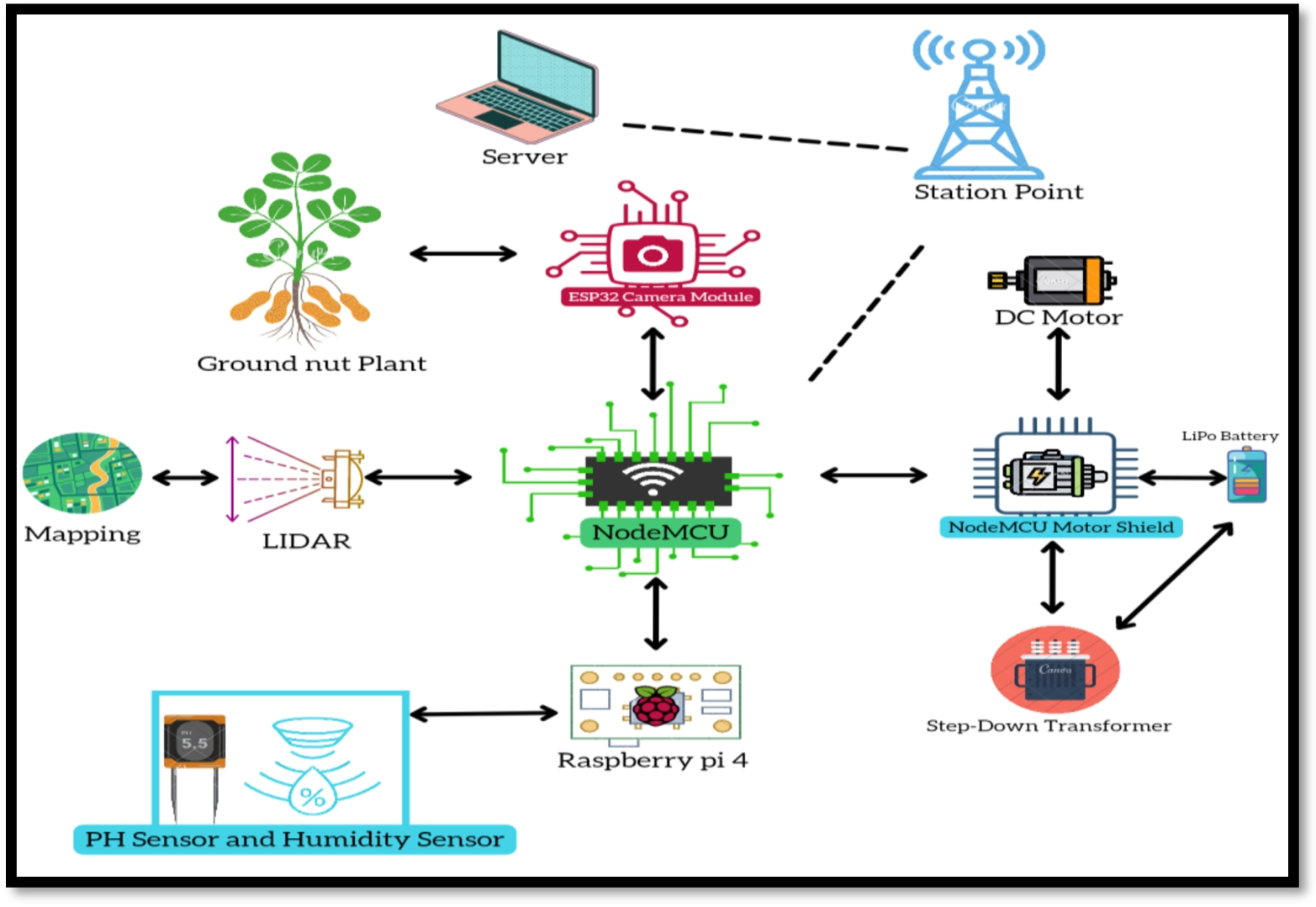
The mobile robot walks with the help of a four-wheeled walking gadget. A brush motor 6V Gear Micro DC Encoder [53] propels each tyre, allows the vehicle to run at speeds of up to 1 m/s and swivel at a rate of 6.6 rad/s. The robotic tyre speed and displacement are measured using 360 line AB 2 phase continuous rotary encoder. A robot platform control scheme and server make up majority of the robot manipulator hardware system. Figure 5 depicts the structural block diagram. A principal processor, a VL53L1X Lidar Sensor, Inertial Measurement Unit (IMU) unit, a location controller, 22.2V LIPO Lithium Polymer Battery power supply module makes the open source robot platform control system. It’s not only proficient of autonomously directing and placing the mobile robot. Object detection and other aspects, as well as the right to receive server software to send commands to direct the robot’s movement and a range of sensor data sent over WIFI to the server. An ESP8266 Node MCU Development Board with 1GB of RAM and a range of connectors, such as a built-in 10/100 dynamic network adapter, an 802.11n WIFI wireless USB network card, and a server wireless network card, serves as main controller (3D printed using PLA material).
The bottom driver board Node MCU and Raspberry pi 4 is the key component of the position control module. The Node MCU Motor Shield will be the speed controller for 366PRM DC brush motor. The Motor Shield measures the speed at which the object moves and the direction of the robot manure is controlled by movement of side wheels. Determine the robot’s orientation, direction, and acceleration in 3D space, you’re moving. Motor Shield employs PID control to enable the robot to interact with the main controller as well as move precisely. The speed, angle, mileage of robot’s wheels determine its location. The main controller uses the VL53L1X Lidar Sensor laser sensor to capture 2D laser data from the environment, then wirelessly transfers it to the server utilizing ROS distributed processing to make a map of world around the robot.
A 22.2V 2800mAh large rechargeable lithium battery powers the mobile robot platform. Three 18650 lithiumion battery packs make up the battery, which is enough to power the complete system. Lenovo Y480 machines are employed on the server. Ubuntu 16.04 and the Free Software Robotics Operating System are installed in a virtual computer (ROS). The mobile robot platform’s principal controller first shifts the robot’s 2D laser data into 3D space, viz, orientation, velocity, distance, robot’s environment. Map of complete unfamiliar part is regularly generated by managing the robot’s behavior at the host.
4.2.Model of software for mobile robots
The trials are carried out in a two-wheel mobile robot equipped with an Intel Core i7-4500U 1.8 GHz CPU, 8 GB of memory, and a Robot Operating System running in a computer equipped with four Intel Core i7 2.2 GHz processors, eight gigabytes of RAM, and an Intel HD Graphics 6000 graphics card. The ROS system framework builds a platform that links all activities and installs the bulk of the key feature modules and packages [25,51], mostly from the ROS community, after install the complete desktop ROS version. By customizing the robot software system to own robot as well as generating more node and processing packaging, the gained general resources may be simply updated to finish the creation of the robot software system. This study takes extensive usage of ROS distributed processing architecture because map development and vehicle location need a significant count of data processing using a single card type computer is difficult. First, the host and the robot head controller are on the same network and are coupled to the same LAN. On the server, construct Node Managers and keyboard trouble shoots, IMU errors, autonomous vehicle linear and angular velocity adjustments, SLAM nodes in mobile robot host controller, Lidar, Odometer, and Base Controller nodes.
The node manager can then employ a peer-to-peer architecture on the current web to execute TCP/IP message and achieve successful nodes on separate hosts can communicate with each other after all of the nodes have been registered and monitored by the node management. Finally, perform the SLAM job on the server in an unknown area using the 3D visualization application RVIZ. The node topology is considered for robots in the ROS system framework. The processes that the RVIZ tool may debug are mostly handled by the server-side node: To implement SLAM and run at RVIZ, obtained objects such as lasers signals and postures from the robot control system laser sensor and odometer node, respectively. There are options in both horizontal and angular velocity adjustments. To improve the precision of adjustment, change the line tempo and its correction codes.
4.3.Programming for point regulator
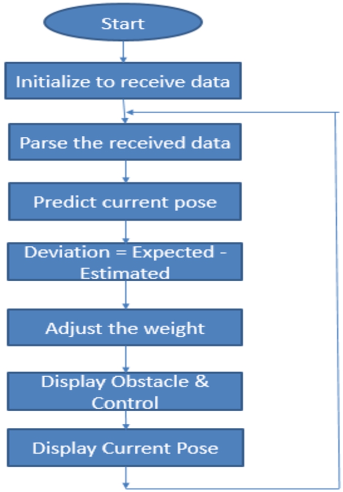
As a node of ROS, the point regulator mode analyses the straight speed with angular velocity data provided through the core processing center, to determine parameters that the robot must be able to move in both wheels. The robot follows the trajectory given by the host’s movement instruction and uses laser distance meter to avoid barrier. Finally, robot communicates the mileage node attitude parameters including flow rate, angular momentum, and movement. Figure 6 shows the flowchart for the software.
Fig. 6.
Programming for point regulator.
5.Experimental results and analysis
Following the software requirements for mobile robots, has been built up, the foundation for SLAM research is Robot movement can be controlled remotely using the ROS shared processing system. As a result, we’ll need to use RVIZ and other visualization apparatuses to remotely manage receive comments from the mobile robot at first. After that, SLAM test can utilized to ensure that design fits the need. IMU on trolley should be measured before wheeled operation, to better place the mobile robot operation is controlled. In this study, the GY-85 9-channel IMU is used. IMU inertial sensing sensor featuring triaxial geomagnetometer, triaxial accelerometer, and triaxial gyroscope [60]. The mobile robot’s IMU passes a multiple tests, and the data is analyzed and the coordinates are determined. The x, y, and z systems of mobile robot have been rectified. Way to take the x, y, z coordinate system is constant. To improve the initial motion estimate, IMU’s fusion with a weighted average the initial position estimation and calculation value were used.
Before trolley procedure is managed, IMU on trolley should be measured in order to enhance position the mobile robot. In this study, the GY-85 9-channel IMU is used. Inertial measurement unit (IMU) sensor with axis gyroscope sensor, the triaxial geomagnetometer, triaxial accelerometer, and triaxial gyroscope [53] are all triaxial devices. The mobile robot’s IMU passes a test. A significant number of coordinates have been determined and the data has been calculated. The mobile robot’s x, y, and z systems have been calibrated. The best way to travel the three axis is to use a coordinate system that is consistent. The IMU as well as the IMU’s weighted average fusion is done to enhance the estimation of starting motion by combine value of initial attitude assessment and the value of the attitude calculation.
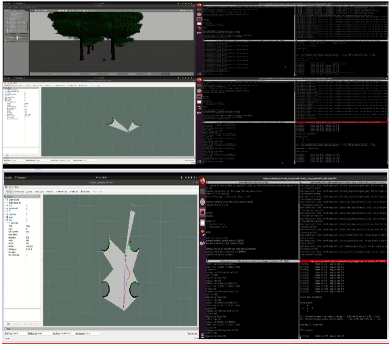
Figure 7: Top left shows simulated environment. Top Right: Generation of Map with initial guess. Bottom Left: Scan Matching with Map update. Bottom Right: Generated map with obstacle detection.
The SLAM code is injected into the Node MCU module. It is connected directly with Node MCU Motor Shield. The battery, DC motors, and Step down Transformer are all connected to the Motor Shield. The voltage supply required by each item is regulated by the Step down Transformer. The Motor shield aids in the management of the motors. For the Lidar to cover a large angle and project in 180°, it is first positioned on top of the stepper motor. The data from the Lidar is then transferred to the Node MCU, where it is mapped inside RVIZ and sent to SLAM for localization. These data are transferred to our server via Node MCU over WIFI. Based on the Lidar data we receive, the Motor shield supplies us with co-ordinates for robot navigation, and therefore obstacles detection occurs. The Node MCU is attached to the camera module, which captures data as we move and sends it to the Raspberry Pi 4, which has our illness classification module.
Fig. 7.
Autonomous navigation on agriculture field.
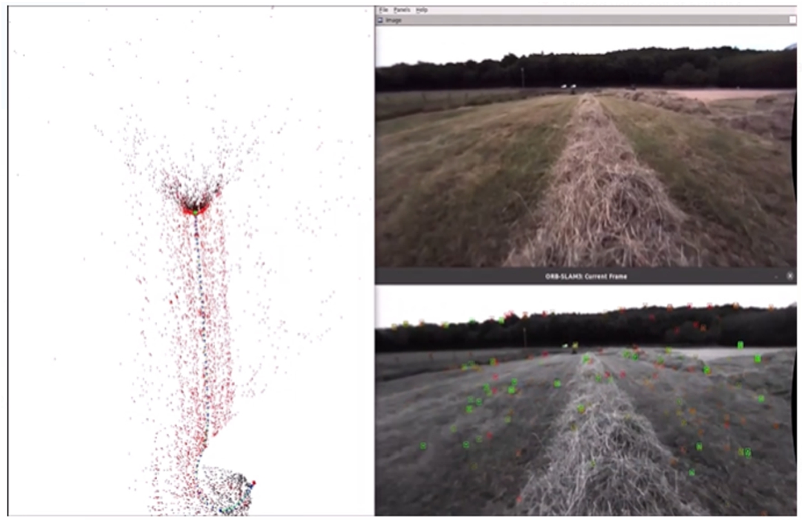
The camera as well as ph and humidity sensors, are mounted on a robot arm to provide leverage for capturing images of leaves and testing the soil in the ground. All of these data are submitted to our server, which then generates a report. Figure 7 represents the simulated environment for testing purpose. It simulates initial guess green color assumed as tree, black color assumed as rigid or boundary, gray color treated as agriculture field, white color dots treated as plants in agriculture field. Tree, boundary, plant are consider as obstacle by the propose algorithm. Semantically organized point cloud data is shown in Fig. 8. Left top shows the camera recording and the left bottom shows corresponding Lidar capturing. Right image displays the generated point cloud data.
Fig. 8.
Semantically organized point cloud data.
Most of the autonomous navigation research used image processing based path planning. Figure 9 depicts the Comparison of generated path with SLAM-HSAStar algorithm, LS Track, and EKF Track. Here black color line represents the proposed hyb SLAM-AStar algorithm track and it shows the shortest path compared with existing tracks such as Link state algorithm (LS) Track, and extended Kalman filter (EKF) Track respectively.
Fig. 9.
Comparison of generated path with SLAM, LS track, and EKF track.
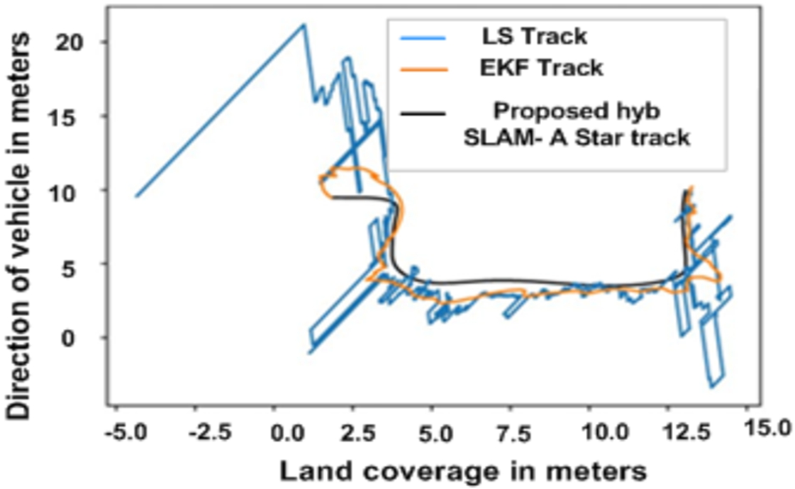
Fig. 10.
Pose estimation of autonomous robot.
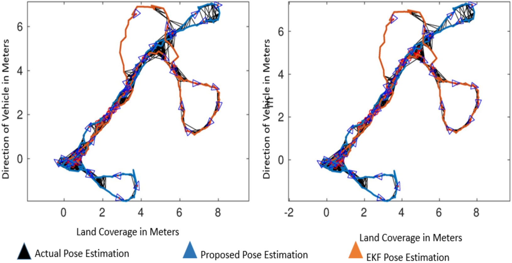
Pose estimation another important measure for autonomous navigation. Figure 10 shows the pose estimation for different trajectory for unknown environment. Pose estimation influences by the temporal for the optimal route taken by the robot. In the above Fig. 10 X and Y axis represented land coverage in meter, in that black color triangles represent the actual pose estimation in unknown environment. Blue color triangles show the proposed algorithm pose estimation in the unknown environment. Ls track means that the path generated only from the Lidar sensor. Orange color triangle shows that state of art algorithm pose estimation in an unknown environment. Form the graph we infer that the proposed algorithm gives the accurate pose estimation in an unknown environment.
6.Discussion
This study looked into modelling and path of a UGV’s persistent monitoring of an unknown environment. A unique occurrence modelling strategy is planned to discretize path, compute the observing effect, and define the model we are concerned about. Simulation analysis and baseline comparison are used to assess the feasibility and correctness of a path planning method. Simulation demonstrates the method’s validity in the case of weighted visits to certain positions.
The findings of simulation studies show a correlation between system characteristics and algorithm performance, indicating that the actual algorithm performance cannot be anticipated precisely under multiple scenarios. Figure 11 shows the simulated environment of agriculture field. The starting robot’s orientation is depicted in this middle photograph in the simulated environment. Bottom image represents autonomous exploration of robot, in that green color shows the visible objects with in a range. Blue color line interprets the estimated expected path for robot, red color line shows actual navigation of robot and gray color region shows exploration without any obstacle.
Fig. 11.
Simulated environment (top). Initial position of robot (middle). Autonomous exploration of robot (bottom).
The following measures are used to assess the quality of a SLAM algorithm: The number of corners in a map, which determines the precision of a map, the percentage of occupied and free cells, which allows one to identify whether obstacle/object on a map are blurred and whether extra obstacle/object developed owing to an algorithm failure. If there are overlapping obstacle/object or artefacts in an unknown location, this measure can be used to detect them, as can the number of enclosed areas, which expresses the same idea. Table 1 shows the three trials of mapping parameter.
Table 1
Three trials of mapping parameter
| Trail | 1 | 2 | 3 |
| Speed of the robot (m/s) | 0.5 | 0.1 | 0.12 |
| Map update interval (s) | 10 | 5 | 3 |
| Particle filter count | 30 | 25 | 20 |
Fig. 12.
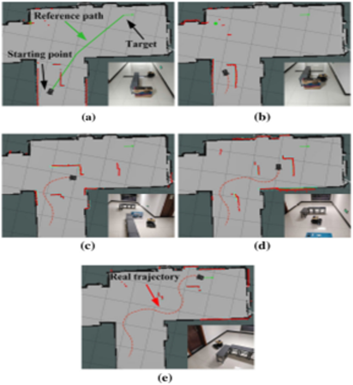
Procedure of robot experimentation (a)–(e) displays robot location at chronological sort.
As a result, it is difficult to come up with a models, there is a common adaptive criterion of the highest reward coefficient. Precision of map is computed, when the robot has done mapping, the accuracy of the map is calculated. The correctness of map is determined using equation (15), which is depends on the total area of the actual map layout. The x shows the complete range of the robot’s map, meanwhile the y reflects the real map’s overall length.
6.1.Experimental scenario map or scenario for some sample trails
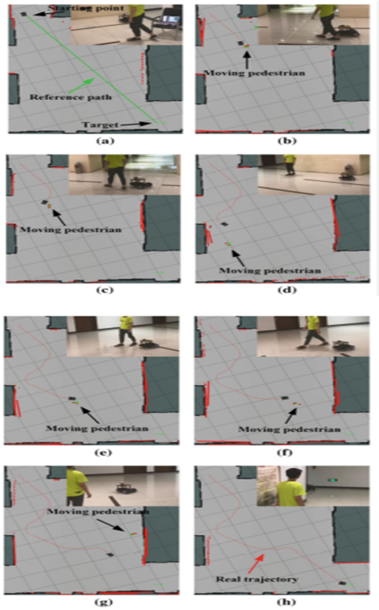
The map or scenario for some sample trails, A star algorithm is upgraded for feasible performance of navigation, then the trained agent is acquired via complex environment having certain trails, trial 1 is given in Fig. 12, trial 2 is given in Fig. 13, trial 3 is given in Fig. 14. The proposed approach handles using the picture including simple changing constraints. Original scenario map fabricated through Simultaneous Localization and Mapping is given in Fig. 13(a), the real environment to navigation is represented in Fig. 13(b). Here, a person randomly walks at scenario who considerably intercepts the robot path twice to target. Figure 14 depicts temporal series of robot navigation snapshots visualized in ROS, viz, related positioning of real robot in experiment. Figure 14(a) portrays initial place, objective and orientation path. Reference path goes straight to goal owing to lack of obstacle in the original map. Figure 14(b)–(g) displays the robot movements averting the moving pedestrian. The robot steers away from this pedestrian when the pedestrian hinders the robot motion (Figs 14(b) to 14(f)). If the person is away from the robot, the robot back to the direction of goal (Figs 14(d), (g)). The real path as robot attains the target is depicted in Fig. 14(e). Here, the real trajectory averts the moving pedestrian, also vary from reference path that exemplifies the proposed approach proficiently navigate the robot in simple dynamic situation.
Fig. 13.
(a): Experiment scenario original map of sample trails 1, (b) real experiment scenario.
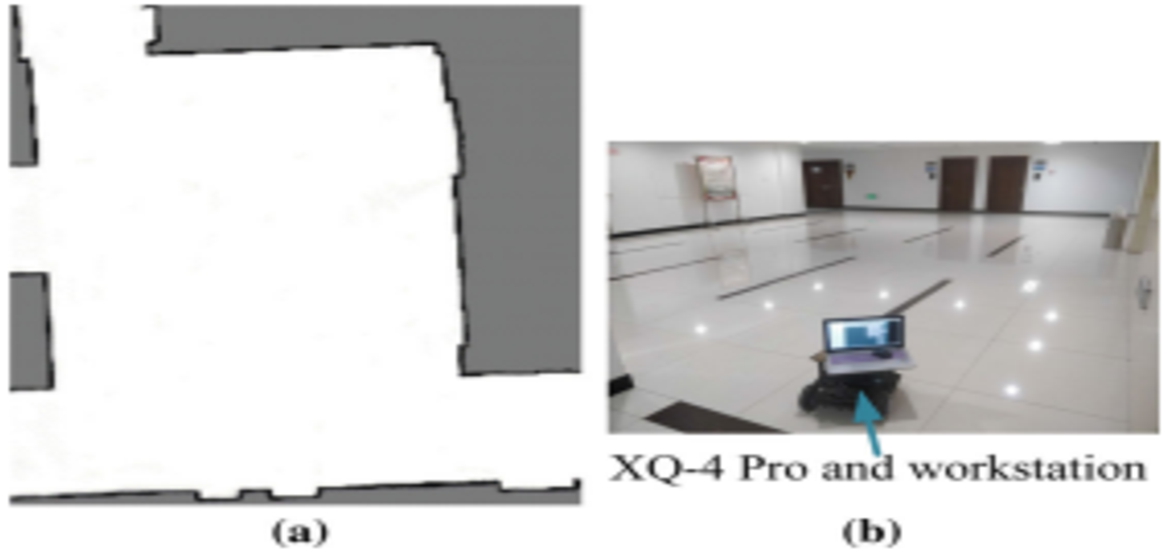
Fig. 14.
Procedure of robot experimentation 2. (a)–(h) displays robot location at chronological sort.
6.2.Performance metrics
Here, the performance measures like accuracy, map size, specificity, patch length, map duration and execution time are looked at in order to assess performance.
6.2.1.Accuracy
Accuracy is described as the total number of instances in the data. As a result, equation (12) determines it,
6.2.2.Map size
Map size depends on the specific application or system being evaluated. It is estimated using equation (13),
6.2.3.Patch length
Patch length is a term used in environmental monitoring to refer to the size of the area that is being sampled or monitored for a particular environmental parameter. The patch length is usually defined as the distance over which the parameter of interest is assumed to be homogeneous and representative of the larger area being monitored. Patch length is estimated using equation (14),
6.2.4.Map duration
Map duration is a term used in environmental monitoring to refer to the length of time over which data is collected at each monitoring location to create a spatial map of the environmental parameter of interest. Map duration is estimated using equation (15) as follows,
6.2.5.Execution time
Execution time is a term used in environmental monitoring to refer to the total amount of time required to complete a monitoring program. The execution time is an important consideration in environmental monitoring, as it affects the overall cost and efficiency of the program.
The execution time can be mathematically defined using the following equation (16),
The map can saved periodically; for the mapping procedure in this study, the SLAM approach is combined with the GMapping algorithm. Three trials with varying robot velocity, map update frequency, and particle filter parameters are established to see how they affect mapping quality. Figure 15 represent the mapping accuracy for different trails. The mapping and navigation process can be observed using the ROS “rviz” interface. Inside the ROS, the multisensory data provided by the RPLIDAR360o laser scanning and two optical progressive encoders were processed. It’s more convenient and quick this way. As it develops, it becomes a method for long-distance navigation and mapping.
Fig. 15.
Accuracy analysis.
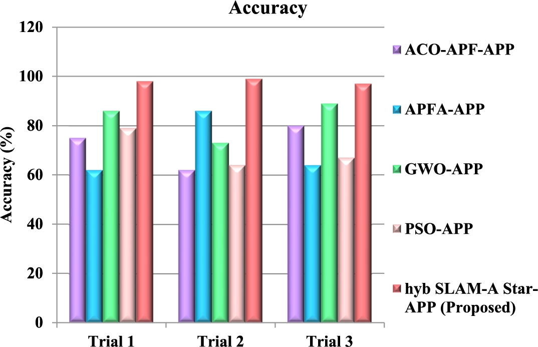
Figure 15 shows the accuracy analysis. The proposed hyb SLAM-A Star-APP method provides 22.35%, 29.67%, and 28.67% higher accuracy for trial 1; 32.56%, 29.06% and 29.05% higher accuracy for trial 2; 25.32%, 35.48% and 54.28% higher accuracy for trial 3 than the existing methods such as ACO-APF-APP, APFA-APP, GWO-APP and PSO-APP respectively.
Figure 16 shows the map size analysis. The proposed hyb SLAM-A Star-APP method provides 23.65%, 29.67%, and 32.56% lower map size for trial 1; 36.52%, 22.17% and 34.89% lower map size for trial 2; 31.08%, 29.63% and 32.56% lower map size for trial 3 than the existing methods such as ACO-APF-APP, APFA-APP, GWO-APP and PSO-APP respectively.
Fig. 16.
Map size analysis.
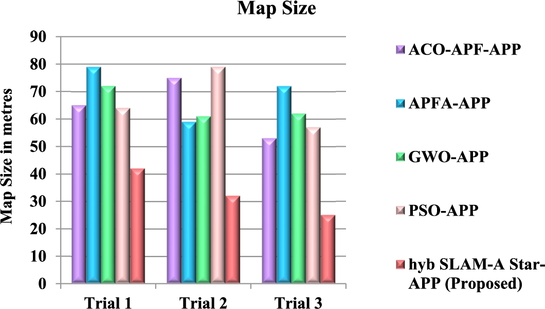
Fig. 17.
Map duration analysis.
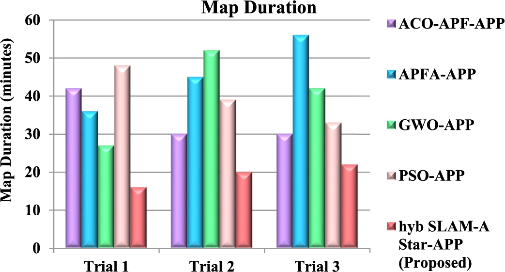
Fig. 18.
Patch length analysis.
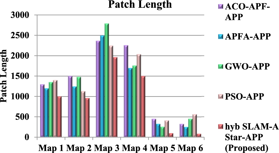
Figure 17 shows the map duration analysis. The proposed hyb SLAM-A Star-APP method provides 36.29%, 27.68%, and 35.68% lower map duration for trial 1; 21.36%, 29.64% and 29.67% lower map duration for trial 2; 41.32%, 30.27% and 42.35% lower map duration for trial 3 than the existing methods such as ACO-APF-APP, APFA-APP, GWO-APP and PSO-APP respectively.
Figure 18 shows the patch length analysis. The proposed hyb SLAM-A Star-APP method provides 23.65%, 29.68%, and 24.58% lower patch length for map 2; 27.38%, 33.21% and 29.68% lower patch length for map 4; 23.65%, 29.36% and 31.05% lower patch length for map 6 than the existing methods such as ACO-APF-APP, APFA-APP, GWO-APP and PSO-APP respectively.
Fig. 19.
Execution time analysis.
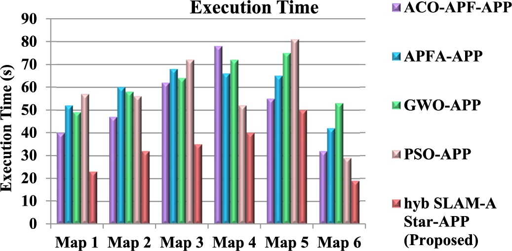
Figure 19 shows the execution time analysis. The proposed hyb SLAM-A Star-APP method provides 32.10%, 29.68%, and 22.47% lower execution time for map 2; 32.15%, 33.21% and 32.10% lower execution time for map 4; 23.10%, 45.36% and 22.10% lower execution time for map 6 than the existing methods, such as ACO-APF-APP, APFA-APP, GWO-APP and PSO-APP respectively.
7.Conclusion
This paper purposes a unique adaptive path planning framework to address a new challenge known as the Unknown environment Persistent Monitoring Problem (PMP) is successfully implemented. To map an unfamiliar location using the robotic operating system (ROS), the 3D visualization tool for Robot Operating System (RVIZ) is utilized, and GMapping software package which is an open access are used for SLAM usage. The experimental results suggest mobile robot design pattern is viable to produce a high-precision map while lowering the cost of the mobile robot SLAM hardware. From a decision-making standpoint, a hybrid algorithm HSAStar (Hybrid SLAM & A Star) algorithm is built for path planning based on the event oriented modelling, allowing a UGV to continually monitor the perspectives of path. The simulation results and analyses show that the proposed strategy is feasible and superior. Then the performance of the proposed hyb SLAM-A Star-APP method provides 27.38%, 33.21% and 29.68% lower execution time, .36%, 29.64% and 29.67% lower map duration is compared with the existing method such as ACO-APF-APP, APFA-APP, GWO-APP and PSO-APP respectively.
7.1.Future work
The proposed algorithm attains more accurate result in terms of map generation, pose estimation in unknown condition. The experiment concludes that the proposed hybrid SLAM-A star algorithm is effectual as well as practical for optimizing motion and velocity in uncertainty. The tuning model hints to certain merits in real-life as well as industrial application, because it save time to novice control engineers to reach ideal motion with velocity in the parameters uncertainties, also enhance the performance superiority. However, it is limited due to high power consumption. In future work, low power consumption robots can be designed and deep learning method with optimization algorithm can be used.
Conflict of interest
None to report.
References
[1] | M.S. Abed, O.F. Lutfy and Q.F. Al-Doori, Online optimization application on path planning in unknown environments, Journal Européen des Systèmes Automatisés 55: (1) ((2022) ), 61–69. doi:10.18280/jesa.55010619. |
[2] | B. Anang, FARM technology adoption by smallholder farmers in Ghana, Review of Agricultural and Applied Economics 21: (2) ((2018) ), 41–47. doi:10.15414/raae.2018.21.02.41-47. |
[3] | P. Atkar, A. Greenfield, D. Conner, H. Choset and A. Rizzi, Uniform coverage of automotive surface patches, The International Journal of Robotics Research 24: (11) ((2005) ), 883–898. doi:10.1177/0278364905059058. |
[4] | C. Baker, R. Rapp, E. Elwakil and J. Zhang, Infrastructure assessment post-disaster: Remotely sensing bridge structural damage by unmanned aerial vehicle in low-light conditions, Journal of Emergency Management 18: (1) ((2020) ), 27–41. doi:10.5055/jem.2020.0448. |
[5] | K. Bergman, O. Ljungqvist, T. Glad and D. Axehill, An optimization-based receding horizon trajectory planning algorithm, IFAC-Papers On Line 53: (2) ((2020) ), 15550–15557. doi:10.1016/j.ifacol.2020.12.2399. |
[6] | K. Bergman, O. Ljungqvist, T. Glad and D. Axehill, An optimization-based receding horizon trajectory planning algorithm, IFAC-PapersOnLine 53: (2) ((2020) ), 15550–15557. doi:10.1016/j.ifacol.2020.12.2399. |
[7] | A. Bircher, M. Kamel, K. Alexis, H. Oleynikova and R. Siegwart, Receding horizon path planning for 3D exploration and surface inspection, Autonomous Robots 42: (2) ((2016) ), 291–306. doi:10.1007/s10514-016-9610-0. |
[8] | A. Blanchard and T. Sapsis, Informative path planning for anomaly detection in environment exploration and monitoring, Ocean Engineering 243: ((2022) ), 110242. doi:10.1016/j.oceaneng.2021.110242. |
[9] | Z. Cao, D. Zhang and M. Zhou, Direction control and adaptive path following of 3-d snake-like robot motion, IEEE Transactions on Cybernetics ((2021) ). doi:10.1109/TCYB.2021.30555. |
[10] | D. Casbeer, D. Kingston, R. Beard and T. McLain, Cooperative forest fire surveillance using a team of small unmanned air vehicles, International Journal of Systems Science 37: (6) ((2006) ), 351–360. doi:10.1080/00207720500438480. |
[11] | Y. Chen, G. Bai, Y. Zhan, X. Hu and J. Liu, Path planning and obstacle avoiding of the USV based on improved ACO-APF hybrid algorithm with adaptive early-warning, IEEE Access 9: ((2021) ), 40728–40742. doi:10.1109/ACCESS.2021.3062375. |
[12] | J. Clark and R. Fierro, Mobile robotic sensors for perimeter detection and tracking, ISA Transactions 46: (1) ((2007) ), 3–13. doi:10.1016/j.isatra.2006.08.001. |
[13] | M. Eich, R. Hartanto, S. Kasperski, S. Natarajan and J. Wollenberg, Towards coordinated multirobot missions for lunar sample collection in an unknown environment, Journal of Field Robotics 31: (1) ((2013) ), 35–74. doi:10.1002/rob.21491. |
[14] | H. Gao, B. Cheng, J. Wang, K. Li, J. Zhao and D. Li, Object classification using CNN-based fusion of vision and LIDAR in autonomous vehicle environment, IEEE Transactions on Industrial Informatics 14: (9) ((2018) ), 4224–4231. doi:10.1109/tii.2018.2822828. |
[15] | H. Gao, H. Yu, G. Xie, H. Ma, Y. Xu and D. Li, Hardware and software architecture of intelligent vehicles and road verification in typical traffic scenarios, IET Intelligent Transport Systems 13: (6) ((2019) ), 960–966. doi:10.1049/iet-its.2018.5351. |
[16] | Y. Girdhar and G. Dudek, Modeling curiosity in a mobile robot for long-term autonomous exploration and monitoring, Autonomous Robots 40: (7) ((2015) ), 1267–1278. doi:10.1007/s10514-015-9500-x. |
[17] | A. Goel, K. Ail, M. Donnellan, A. Gomez de Silva Garza and T. Callantine, Multistrategy adaptive path planning, IEEE Expert 9: (6) ((1994) ), 57–65. doi:10.1109/64.363273. |
[18] | U. Goel, S. Varshney, A. Jain, S. Maheshwari and A. Shukla, Three dimensional path planning for UAVs in dynamic environment using glow-worm swarm optimization, Procedia Computer Science 133: ((2018) ), 230–239. doi:10.1016/j.procs.2018.07.028. |
[19] | L. Haibo, D. Shuliang, L. Zunmin and Y. Chuijie, Study and experiment on a wheat precision seeding robot, Journal of Robotics 2015: ((2015) ), 1–9. doi:10.1155/2015/696301. |
[20] | G. Hitz, E. Galceran, M. Garneau, F. Pomerleau and R. Siegwart, Adaptive continuous-space informative path planning for online environmental monitoring, Journal of Field Robotics 34: (8) ((2017) ), 1427–1449. doi:10.1002/rob.21722. |
[21] | G. Hitz, E. Galceran, M. Garneau, F. Pomerleau and R. Siegwart, Adaptive continuous-space informative path planning for online environmental monitoring, Journal of Field Robotics 34: (8) ((2017) ), 1427–1449. doi:10.1002/rob.21722. |
[22] | G. Huang, Z. Liu, G. Pleiss, L. Van Der Maaten and K. Weinberger, Convolutional networks with dense connectivity, IEEE Transactions on Pattern Analysis and Machine Intelligence ((2019) ), 1–1. doi:10.1109/tpami.2019.2918284. |
[23] | ICRA ’07–2007 IEEE international conference on robotics and automation, IEEE Robotics & Automation Magazine 13: (1) ((2006) ), 93–93. doi:10.1109/mra.2006.1598062. |
[24] | A. Johnson and M. Hebert, Seafloor map generation for autonomous underwater vehicle navigation, Autonomous Robots 3: (2–3) ((1996) ), 145–168. doi:10.1007/bf00141152. |
[25] | D. Kaur and B. Velayudhan, Microcontroller-driven gray scale plasma receiver, Journal of Microcomputer Applications 18: (1) ((1995) ), 55–64. doi:10.1016/s0745-7138(95)80022-0. |
[26] | W. Khaksar, T. Hong, M. Khaksar and O. Motlagh, Sampling-based tabu search approach for online path planning, Advanced Robotics 26: (8–9) ((2012) ), 1013–1034. doi:10.1163/156855312x632166. |
[27] | A. Kolling, A. Kleiner and S. Carpin, Coordinated search with multiple robots arranged in line formations, IEEE Transactions on Robotics 34: (2) ((2018) ), 459–473. doi:10.1109/tro.2017.2776305. |
[28] | D. Li and H. Gao, A hardware platform framework for an intelligent vehicle based on a driving brain, Engineering 4: (4) ((2018) ), 464–470. doi:10.1016/j.eng.2018.07.015. |
[29] | L. Liu, X. Xia, H. Sun, Q. Shen, J. Xu, B. Chen, H. Huang and K. Xu, Object-aware guidance for autonomous scene reconstruction, ACM Transactions on Graphics 37: (4) ((2018) ), 1–12. doi:10.1145/3197517.3201399. |
[30] | R. Liu, Improved ant colony algorithm-based automated guided vehicle path planning research for sensor-aware obstacle avoidance, Sensors and Materials 33: (8) ((2021) ), 2679. doi:10.18494/SAM.2021.3396. |
[31] | W. Liu, Slam algorithm for multi-robot communication in unknown environment based on particle filter, Journal of Ambient Intelligence and Humanized Computing ((2021) ). doi:10.1007/s12652-021-03020-3. |
[32] | S. Mohanty, D. Hughes and M. Salathé, Using deep learning for image-based plant disease detection, Frontiers in Plant Science 7: ((2016) ). doi:10.3389/fpls.2016.01419. |
[33] | H. Mouhagir, V. Cherfaoui, R. Talj, F. Aioun and F. Guillemard, Trajectory planning for autonomous vehicle in uncertain environment using evidential grid, IFAC-PapersOnLine 50: (1) ((2017) ), 12545–12550. doi:10.1016/j.ifacol.2017.08.2193. |
[34] | R. Mur-Artal, J. Montiel and J. Tardos, ORB-SLAM: A versatile and accurate monocular SLAM system, IEEE Transactions on Robotics 31: (5) ((2015) ), 1147–1163. doi:10.1109/tro.2015.2463671. |
[35] | L. Oliveira, A. Moreira and M. Silva, Advances in agriculture robotics: A state-of-the-art review and challenges ahead, Robotics 10: (2) ((2021) ), 52. doi:10.3390/robotics10020052. |
[36] | P. Pach, Monochromatic solutions to |
[37] | PC controlled autonomous navigation system for GPS guided field robot, Journal of Biosystems Engineering 34: (4) ((2009) ), 278–285. doi:10.5307/jbe.2009.34.4.278. |
[38] | M. Popović, T. Vidal-Calleja, G. Hitz, J.J. Chung, I. Sa, R. Siegwart and J. Nieto, An informative path planning framework for UAV-based terrain monitoring, Autonomous Robots 44: (6) ((2020) ), 889–911. doi:10.1007/s10514-020-09903-2. |
[39] | P. Rajesh, S. Muthubalaji, S. Srinivasan and F.H. Shajin, Leveraging a dynamic differential annealed optimization and recalling enhanced recurrent neural network for maximum power point tracking in wind energy conversion system, Technology and Economics of Smart Grids and Sustainable Energy. 7: (1) ((2022) ), 1–5. doi:10.1007/s40866-022-00144-z. |
[40] | P. Rajesh, F.H. Shajin and K. Cherukupalli, An efficient hybrid tunicate swarm algorithm and radial basis function searching technique for maximum power point tracking in wind energy conversion system, Journal of Engineering, Design and Technology. ((2021) ). doi:10.1108/JEDT-12-2020-0494. |
[41] | S. Rathinam, Z. Kim and R. Sengupta, Vision-based monitoring of locally linear structures using an unmanned aerial vehicle, Journal of Infrastructure Systems 14: (1) ((2008) ), 52–63. doi:10.1061/(ASCE)1076-0342(2008)14:1(52). |
[42] | I. Rekleitis, J. Bedwani, E. Dupuis, T. Lamarche and P. Allard, Autonomous over-the-horizon navigation using LIDAR data, Autonomous Robots 34: (1–2) ((2012) ), 1–18. doi:10.1007/s10514-012-9309-9. |
[43] | L. Santos, A. Aguiar, F. Santos, A. Valente and M. Petry, Occupancy grid and topological maps extraction from satellite images for path planning in agricultural robots, Robotics 9: (4) ((2020) ), 77. doi:10.3390/robotics9040077. |
[44] | P. Sapaty, M. Sugisaka and T. Ito, Towards unified human-robotic societies, in: Proceedings of International Conference on Artificial Life and Robotics, Vol. 22: , (2017) , pp. 540–544. doi:10.5954/icarob.2017.is-5. |
[45] | F.H. Shajin and P. Rajesh, FPGA realization of a reversible data hiding scheme for 5G MIMO-OFDM system by chaotic key generation-based paillier cryptography along with LDPC and its side channel estimation using machine learning technique, Journal of Circuits, Systems and Computers. 31: (05) ((2022) ), 2250093. doi:10.1142/S0218126622500931. |
[46] | F.H. Shajin, P. Rajesh and M.R. Raja, An efficient VLSI architecture for fast motion estimation exploiting zero motion prejudgment technique and a new quadrant-based search algorithm in HEVC, Circuits, Systems, and Signal Processing. 41: (3) ((2022) ), 1751–1774. doi:10.1007/s00034-021-01850-2. |
[47] | T. Shibata, 2016 IEEE/RSJ international conference on intelligence robots and systems (IROS 2016), Journal of the Robotics Society of Japan 35: (2) ((2017) ), 122–122. doi:10.7210/jrsj.35.122. |
[48] | A. Sintov, A. Borum and T. Bretl, Motion planning of fully actuated closed kinematic chains with revolute joints: A comparative analysis, IEEE Robotics and Automation Letters 3: (4) ((2018) ), 2886–2893. doi:10.1109/lra.2018.2846806. |
[49] | J. Song and K. Byun, Design and control of a four-wheeled omnidirectional mobile robot with steerable omnidirectional wheels, Journal of Robotic Systems 21: (4) ((2004) ), 193–208. doi:10.1002/rob.20009. |
[50] | I. Sucan, M. Moll and L. Kavraki, The open motion planning library, IEEE Robotics & Automation Magazine 19: (4) ((2012) ), 72–82. doi:10.1109/mra.2012.2205651. |
[51] | Tencarva machinery invests in Nashville, Pump Industry Analyst 2014: (8) ((2014) ), 13. doi:10.1016/s1359-6128(14)70329-5. |
[52] | V.P. Tran, F. Santoso and M.A. Garratt, Adaptive trajectory tracking for quadrotor systems in unknown wind environments using particle swarm optimization-based strictly negative imaginary controllers, IEEE Transactions on Aerospace and Electronic Systems 57: (3) ((2021) ), 1742–1752. doi:10.1109/TAES.2020.3048778. |
[53] | L. Wang, T. Zhang, L. Ye, J. Li and S. Su, An efficient calibration method for triaxial gyroscope, IEEE Sensors Journal 21: (18) ((2021) ), 19896–19903. doi:10.1109/jsen.2021.3100589. |
[54] | K. Xu, L. Zheng, Z. Yan, G. Yan, E. Zhang, M. Niessner, O. Deussen, D. Cohen-Or and H. Huang, Autonomous reconstruction of unknown indoor scenes guided by time-varying tensor fields, ACM Transactions on Graphics 36: (6) ((2017) ), 1–15. doi:10.1145/3130800.3130808. |
[55] | Y. Xu, R. Zheng, M. Liu and S. Zhang, CRMI: Confidence-rich mutual information for information-theoretic mapping, IEEE Robotics and Automation Letters 6: (4) ((2021) ), 6434–6441. doi:10.1109/lra.2021.3093023. |
[56] | B. Yamauchi, A frontier-based approach for autonomous exploration, in: Proceedings 1997 IEEE International Symposium on Computational Intelligence in Robotics and Automation CIRA’97.‘Towards New Computational Principles for Robotics and Automation’, (1997) , pp. 146–151, IEEE. doi:10.1109/CIRA.1997.613851. |
[57] | J. Yu, S. Karaman and D. Rus, Persistent monitoring of events with stochastic arrivals at multiple stations, IEEE Transactions on Robotics 31: (3) ((2015) ), 521–535. doi:10.1109/tro.2015.2409453. |
[58] | S. Zhang, S. Zhang, C. Zhang, X. Wang and Y. Shi, Cucumber leaf disease identification with global pooling dilated convolutional neural network, Computers and Electronics in Agriculture 162: ((2019) ), 422–430. doi:10.1016/j.compag.2019.03.012. |
[59] | T. Zhang, C. Wang, Z. Yuan and M. Zheng, Improved grid mapping technology based on Rao-Blackwellized particle filters and the gradient descent algorithm, Systems Science & Control Engineering 7: (1) ((2019) ), 65–74. doi:10.1080/21642583.2019.1566858. |
[60] | X. Zhang, J. Lai, D. Xu, H. Li and M. Fu, 2D lidar-based SLAM and path planning for indoor rescue using mobile robots, Journal of Advanced Transportation 2020: ((2020) ), 1–14. |


