
RECITE: A framework for user trajectory analysis in cultural sites
Abstract
The Internet of Things (IoT) has recently been applied in the domain of cultural exhibition enabling the cultural sites to provide more personal and proactive experiences to their visitors. To come up with valuable services, several solutions to analyze the spatio-temporal trajectories of visitors have been put forward. However, they neither consider the inherent uncertainty of the underlying indoor positioning technologies – Bluetooth Low Energy (BLE), RFID, etc. – nor other visitors’ features apart from the spatio-temporal ones (e.g. the level of interaction with the museum displays). For that reason, the present work introduces RECITE, a framework to classify trajectories representing visitors’ actions that copes with the aforementioned limitations of existing solutions. Firstly, RECITE states a novel mapping process for a BLE-based indoor positioning system to accurately detect the visitors’ locations. On top of this mechanism, RECITE includes an ensemble of fuzzy rule classifiers able to tag the visitors’ ongoing trajectories in real time considering both spatio-temporal and other behavioural factors. Finally, the framework has been evaluated in a case of use scenario showing quite promising results.
1.Introduction
The advent of the Internet of Things (IoT) has come with the development of several indoor location solutions based on different wireless technologies like WiFi [37], RFID [3,18] or Bluetooth Low Energy (BLE) [17]. One of the most prominent applications of these location technologies has been the development of location-based services (LBSs) able to adapt to users’ locations inside buildings [6], provide users with ambient intelligence [19] or detect incidents in road infrastructures [4]. In this context, several proposals have recently arisen in the cultural environment in order to profit from such IoT advances. Some examples are recommendation systems to proactively display personalized content to enhance the visitors’ experience in museums [2] or the active involvement of visitors in public exhibitions [29].
An important consequence of this widespread deployment of LBSs is that, now, cultural institutions have access to an unprecedented amount of visitors’ movement data. As a result, several solutions have successfully applied different data mining techniques over such indoor trajectories so as to come up with innovative cultural services [28]. For instance, several works have made use of clustering techniques to group trajectories sharing certain features [23,24,32] whereas pattern mining techniques have been applied to uncover general flows or trends [38,39]. However, we have observed meaningful limitations when it comes to perform classification analysis of such movement data.
On the one hand, although some classification algorithms have been proposed to particularly deal with indoor trajectories in cultural spaces [22], they relied on trajectory models based on sequences of Points of Interest (POIs) or building elements (e.g rooms, corridors) that individuals have gone through during their visits [25]. This high-level modelling actually hampers the realization of profound analyses in order to deeply understand how visitors behave in a particular cultural space, due to a lack of mobility details. For instance, using a POI-based trajectory representation, we may know that a visitor has been close to a certain spot but not how he has actually moved around that spot. Furthermore, this representation strongly depends on the current spatial distribution POIs. The same applies when using trajectories based on building elements.
On the other hand, indoor trajectories are usually noisy and imprecise due to multiple factors [10]. This makes it difficult to establish crisp boundaries defining the actual movement of users in this type of environments. Existing solutions generally do not take into account such problems during the classification process. They will have an impact on the classification accuracy though.
In this context, the work at hand introduces RECITE, a framework for user trajectory analysis in cultural sites for the provisioning of innovative LBSs. RECITE takes into consideration the aforementioned limitations and flaws of existing solutions and presents a novel approach to classify indoor trajectories based on fuzzy rules [40]. This type of rules has good skills to deal with the noisy and inaccurate locations from indoor positioning systems. In that sense, the present work states a data-driven modelling to generate a set of fuzzy rule classifiers (FRCs) for indoor trajectories in cultural sites.
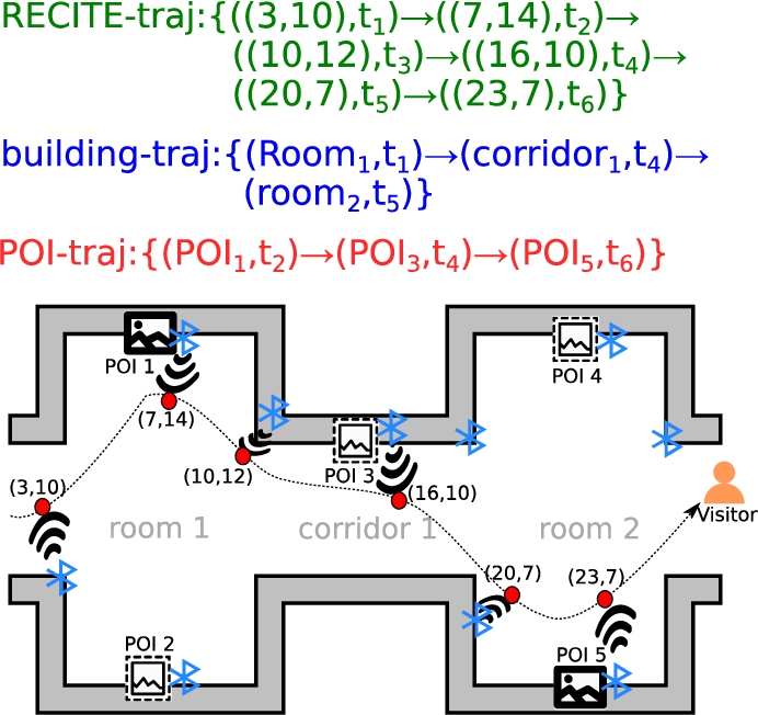
Furthermore, an ad-hoc indoor positioning system based on low-cost BLE beacons has been developed. This system is able to accurately locate users handling a guidance device (e.g. audio-guide) withing a 2-D Cartesian space. Besides, each trajectory is enriched with the interactions that the target visitor made with his device (e.g. play some audio content) during his stay. This way, this type of valuable data can be integrated in the classification process. For the sake of clarity, Fig. 1 shows the difference between our trajectory model and the POI and building-based ones.
Fig. 1.
Examples of POI-based (shown in red), building-element-based (blue) and RECITE (green) indoor trajectories for the same visitor’s displacement in a exhibition scenario with two rooms and one corridor housing five different POIs. The blue icons represent the locations of BLE beacons in the scenario. The red points represent the coordinates in the Cartesian space detected by the our solution.
All in all, to the best of the authors knowledge, this work constitutes one of the first efforts to apply fuzzy rules to classify semantically-enriched indoor trajectories focused on the cultural domain.
The remainder of the paper is structured as follows. Section 2 is devoted to describe in detail the logic structure and the processing stages of RECITE. Then, Section 3 discusses the main results of the performed experiments. Next, an overview about indoor trajectory analysis in the cultural domain is put forward in Section 4. Finally, the main conclusions and the future work are summed up in Section 5.
2.The RECITE framework
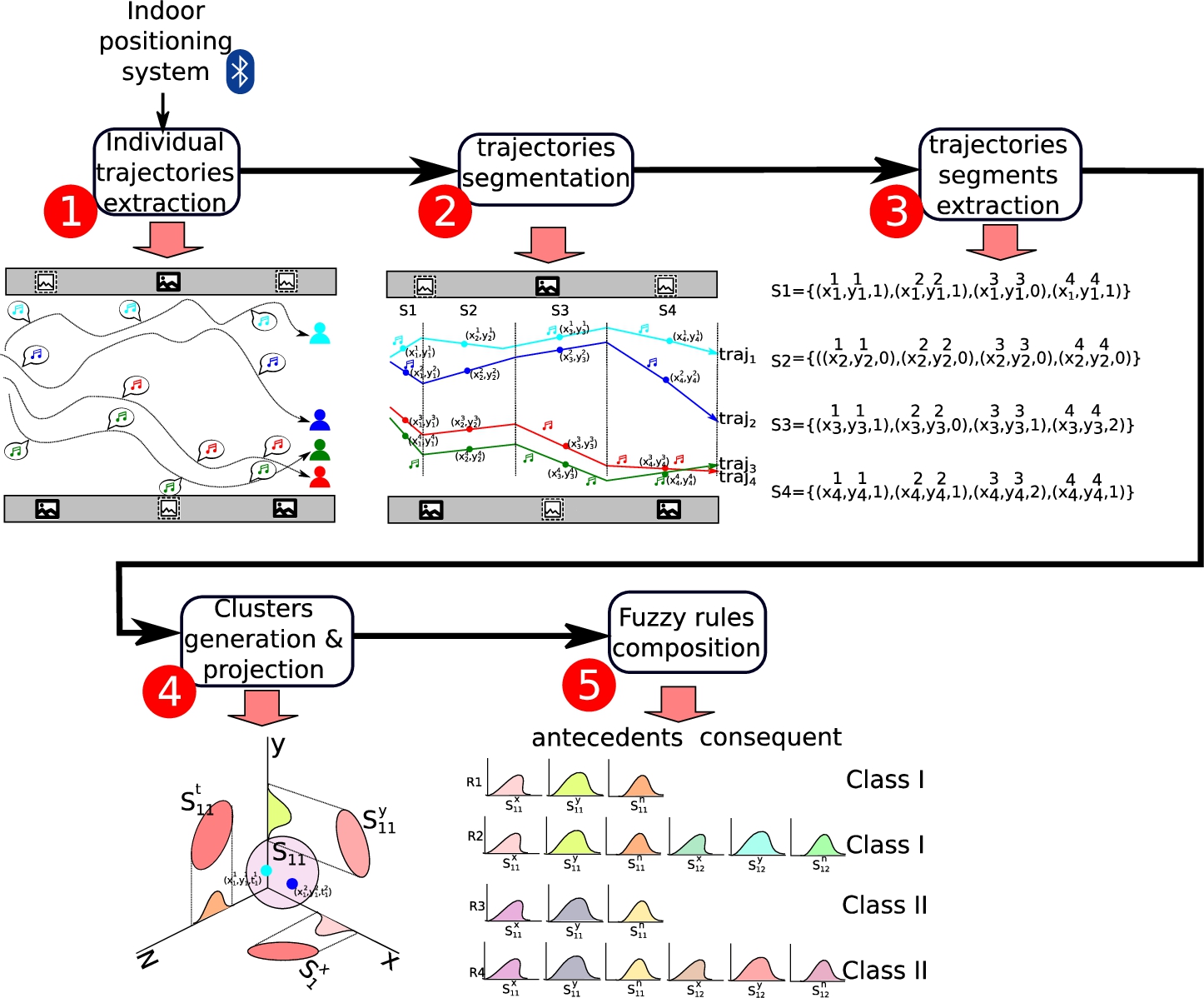
Figure 2 outlines the main steps of RECITE to come up with the proposed FRCs. The first step focuses on collecting the individual trajectories of the museum visitors in terms of spatio-temporal displacements along with the multimedia content displayed by visitors in their guidance devices during such movements. Then, in stage 2, the collected trajectories are split into a pre-defined number of segments (4 in the example of the figure). The third step extracts the overall features of each trajectory segment. In the fourth step, several fuzzy clustering tasks are applied to the data set, but taking into account only a segment and a class at a time. After that, for every clustering model their resulting clusters are projected to their space axis (Cartesian coordinates,
Fig. 2.
Approach overview. As an illustrative example, in the first stage, four different trajectories are collected from visitors where each musical note indicates the location where the user displayed some multimedia content in his handheld device. In stage 2, these input trajectories are split into four segments
2.1.Underlying architecture
RECITE relies on an underlying operational architecture that enables the collection of the required visitors’ behavioural data. Figure 3 shows such an architecture. Bearing this figure in mind, we can derive the following general assumptions for the framework,
Fig. 3.
General operational architecture for RECITE.
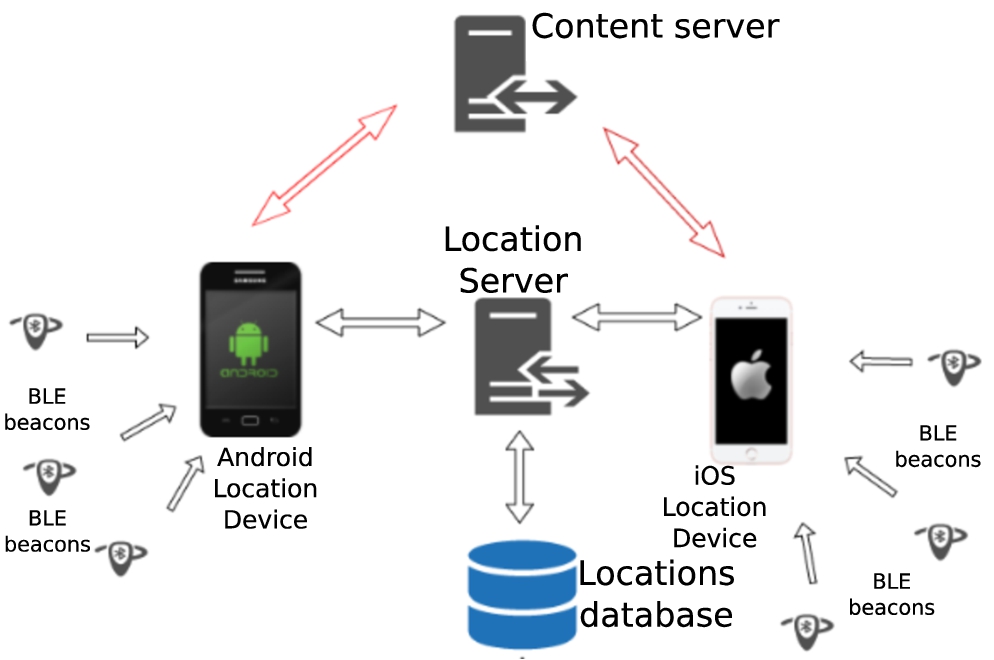
– The museum includes, as part of its own infrastructure, a set of BLE beacons installed through all its exhibition areas (e.g. galleries, corridors and the like). Furthermore, each beacon is identified by means of a unique tag.
– A visitor handles a guidance device during all her/his stay at the museum. The goal of this device is twofold. To begin with, it acts as a Bluetooth-based location system because it is able to periodically detect its closest BLE beacons along with the distance to them. Secondly, it allows the visitor to access the multimedia content related to any exhibition item at the museum.
– The multimedia content is actually stored in a dedicated back-end Content Server accessed by the visitors’ devices on demand. This content might be video, audio or text files providing information about the different museum pieces.
2.2.The classification task
The objective of this work is to obtain an automatic mechanism in such a way that, every given trajectory is classified as one among a set of p predefined labels or classes. Let it be
2.3.Individual trajectories extraction
The first stage of the framework pipeline focuses on collecting the individual trajectories of visitors using the BLE beacons installed in the museum as Fig. 2 shows. In that sense, a visitor’s trajectory can be defined as follows,
Definition 1.
A trajectory
As we can see, RECITE defines a trajectory comprising two types of actions that a visitor can make during his stay,
– Movement actions indicating physical displacements in the museum space.
– Content actions representing interactions with the multimedia content accessible from the guidance device.
In the following sections we describe how these two types of actions are collected.
2.3.1.Movement actions
To capture these actions, the guidance device of a visitor v regularly sends to the Location Server (LS) a frame
In order to process this information, the LS makes use of the museum’s floor-plan image, that is a 2-D Cartesian space where the coordinates of the visitor’s location will be defined. Therefore, the LS performs a mapping process to translate the set of beacon’s distances
1. Dataset generation: This first step is done only once for any new museum where RECITE is going to be deployed. To build the map-like dataset we must associate a scanned frame
2. Comparative inference: In this step, we compare the current frame
Fig. 4.
Illustrative example of the map-based algorithm steps in an scenario with four deployed BLE beacons. The left image shows the data set generation, where the scanner samples the beacons’ signals for certain locations. Only location frames 1 to 3 (
Lastly, in certain situations the guidance devices are not able to capture the signal of a nearby beacon
2.3.2.Content actions
These actions are sent from the visitor’s device to the LS as well. In this case, the device just sends the time-stamp at which the user displayed certain content, together with its associated content identifier.
Each new movement or content action from a visitor is appended to its ongoing trajectory by the LS. In that sense, a trajectory is considered finished when the LS does not receive any new update during a certain time threshold
Lastly, each trajectory is labelled, manually or semi-automatically, with one of the classes in Ω. As a result, a set
2.4.Trajectory segmentation
One of the problems of the previous gathering process is that the sequences of actions defining the trajectories may have varying lengths. Hence, the second step of the framework pipeline is to apply a segmentation process to all the trajectories in
In that sense, trajectory segmentation is a well-known technique in the trajectory data mining field that divides a trajectory into fragments by several criteria, like time intervals or semantic meaning, for further processing [42].
In our setting, trajectories are split into slices of a predefined time length
Definition 2.
A segment of a visitor trajectory
We can see that
Once the different trajectory segments have been composed, they are distributed into different sets
For example, let us consider a trajectory
2.5.Segments feature extraction
Once the trajectory segments have been generated, the next step is to extract a set of descriptive features of each of them. In that sense, depending on the type of action (movement or content display) under consideration, a different type of feature is calculated. As a result, each trajectory segment is compressed into a 3-dimension vector
Definition 3.
A trajectory segment feature
Besides, all the trajectory segment features are collected in their corresponding set
Going back to our previous illustrative trajectory
2.6.Clusters generation and projection
The fourth step of the framework pipeline is to identify the general action trends per segment by means of the generation of different sets of clusters. Every cluster will become a fuzzy rule, and the fuzzy rules will be combined into fuzzy classifiers (see Fig. 2).
The approach is based on the generation of a set of FRCs for every
In this phase, the fuzzy c-means (FCM) clustering algorithm [8] is applied. Before explaining that step, let us give some details about the clustering settings:
– Cluster shape: we decide to obtain hyper-spherical clusters given that they are more suitable to be projected into one dimension fuzzy sets to form fuzzy it-then rules. For more information look for the so-called decomposition error in [5]. This shape is possible when we fix the norm matrix A which induces the measurement dissimilarity between data points as
– Fuzziness: We need to decide the level of overlapping of the fuzzy clusters to be found. This parameter is called m.
– Number of clusters to be identified in every space
– Termination parameter: We need to decide the tolerance threshold ϵ for the FCM algorithm.
Our instance of the FCM algorithm generates
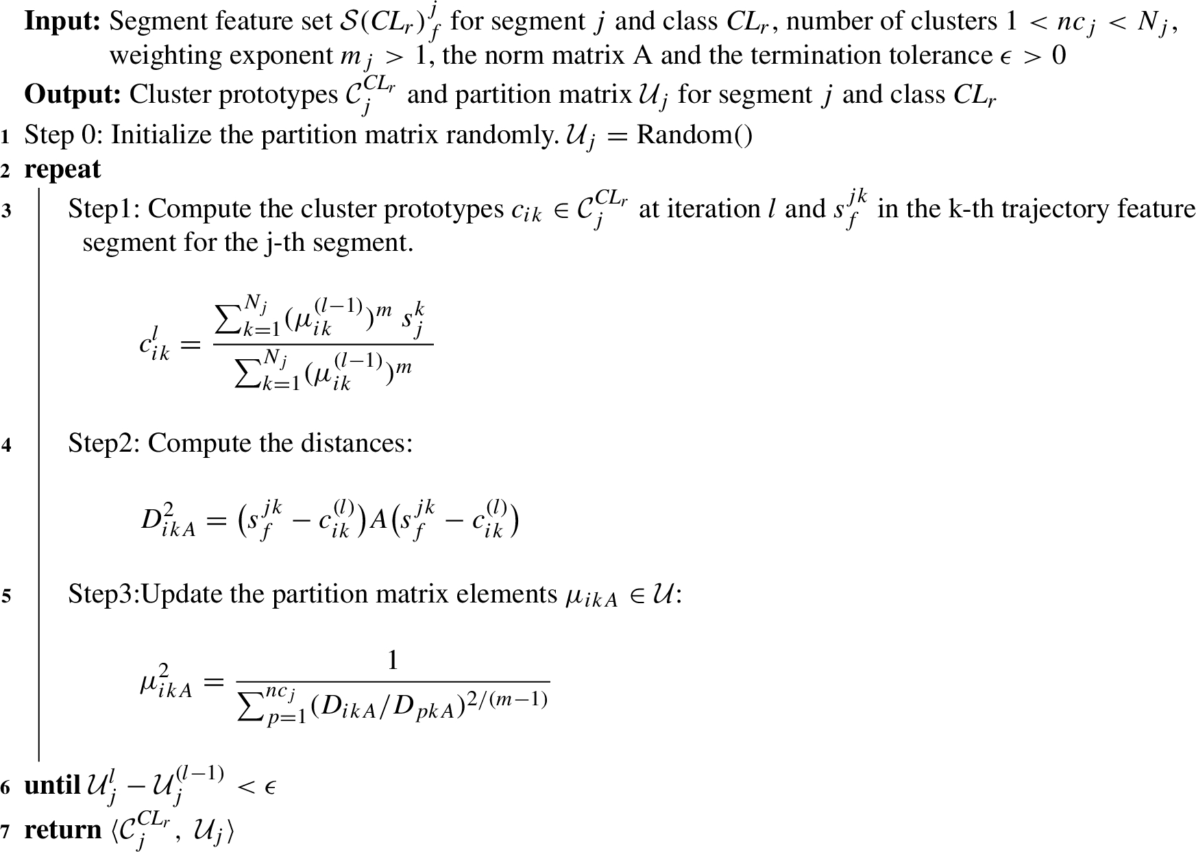
For the sake of completeness, the pseudo-code of the FCM algorithm is included in Algorithm 1 where l indicates the iteration number, i the i-th cluster and k the k-th trajectory segment feature for a particular trajectory segment.
Algorithm 1:
Fuzzy c-means (FCM) algorithm
To obtain the fuzzy sets involved in a fuzzy classifier for class
2.7.Fuzzy classifier composition
At this point we should recall that we carried out clustering tasks based on data of every particular class
Table 1
Fuzzy rule classifier
| IF |
| … AND |
| THEN |
| IF |
| … AND |
| THEN |
| … |
| IF |
| … AND |
| THEN |
– The first step is to calculate the firing strength
– then, the partial output of every rule,
– and the partial outputs are combined to generate the final output
2.7.1.Online classification mechanism
We should recall that the ultimate goal of the classifier is to label the ongoing trajectories of visitors during their stay at a museum. Due to the time-based segmentation described in Section 2.4, these target trajectories will have an increasing number of segments as time proceeds and visitors move across the museum.
In order to cope with this situation, instead of a monolithic FRC, we generate a palette of FRCs with different number fuzzy sets in their antecedents
All in all, the classification mechanism to label the visitors’ ongoing trajectories involves the following steps,
1. Each time a new tuple
2. Then, the
3. Finally,
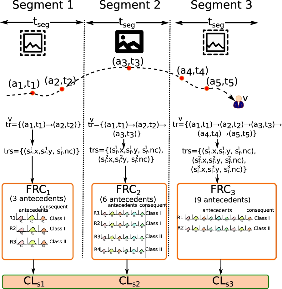
Figure 5 shows an illustrative example of the aforementioned mechanism where a trajectory covers different time-based segments and, thus, feeds different FRCs. As the figure depicts, the target trajectory is labelled with different classes
Fig. 5.
Example of the online classification procedure.
3.Use case
The proposed framework has been evaluated in a test-bed exhibition area. This is located in Murcia, Spain and it usually hosts small exhibitions of local artists.
3.1.Place infrastructure
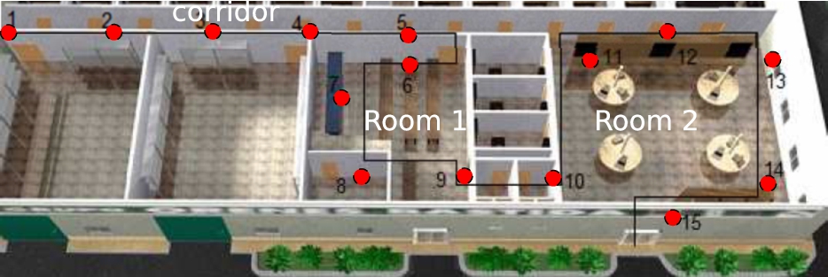
The exhibition place comprises two main rooms distributed along a corridor. In the rooms and the corridor, 15 iBeacons Wellcore W902 with chip TICC254111 were installed as BLE beacons.
Figure 6 depicts the floor-plan of the test-bed along with the spatial distribution of the beacons. Such area covered roughly 500 m2 and the beacons are spatially distributed every 6 meters approximately. The size of this floor-plan image is 500 × 177 pixels and each pixel represents 0.1 m2.
In order to perform the experiment in the test-bed exhibition, we installed the ad-hoc mobile application infoArt in the different guidance devices of the exhibition area.22 This application has two main features,
– Firstly, the app connects to a Content Server to provide visitors with the multimedia content available at the target museum.
– In addition to that, the application generates the BLE frames f every 3 seconds and sends them to the Location Server (LS) (see Fig. 3).
Fig. 6.
Use case floor plan. The red dots indicate the location of the BLE beacons. The black line depicts the ideal route to visit the exhibition area.
3.2.Location algorithm study
As an alternative to the algorithm to detect the movement actions described in Section 2.3.1, we developed a simple mapping approach along with a calibration mechanism to improve its accuracy in our testbed. This was coined as the MinMax location algorithm. In the next two subsections, we state the main findings of our study with respect the algorithm (Section 3.2.1) and the calibration technique (Section 3.2.2).
3.2.1.MinMax location algorithm
This alternative algorithm profited from the fact that we know the euclidean distance to each beacon for every coordinate in our 2-D Cartesian map image. Therefore, for each incoming frame
Nevertheless, this approach suffered from the fact that our handheld guidance devices usually did not sample the same signal strength at the same distance to the transmitter. Consequently, we decided to include a calibration model for each beacon. The goal of this model was to reduce as much as possible the difference between the distance calculated by a guidance device to a beacon and the physical distance between the device and the beacon. This calibration mechanism in described in the next subsection.
3.2.2.Calibration of the beacons
In order to perform the required calibration of the guidance devices, as pointed out above, we took the following steps,
1. First of all, we gathered the signal intensity of each of the 15 deployed beacons in the setting with each guidance device at different displacements covering 1, 2.5, 5, 7.5, 10 and 15 meters. For each of those displacements, we gathered a total of 20 samples.
2. Next, a third-party BLE library,44 integrated in our infoArt application, determined the distance to each beacon based on the collected signal intensities.
3. We averaged the resulting distances per beacon after 5, 10 and 20 samples. This was done because the signal intensity tends to stabilize after several samples [30].
4. On the basis of the previously-calculated distances, a polynomial regression model is generated. This model was used by the application to estimate more precisely the distance to each beacon.
Table 2 shows an example of this calibration process for beacon
Table 2
Example of the mean distance calculated for beacon
| Beacon | Num. of measurements | ||
| Real distance | 5 | 10 | 20 |
| 1 m | 0.66 | 0.6 | 0.62 |
| 2.5 m | 2.67 | 2.88 | 2.98 |
| 5 m | 4 | 4 | 4 |
| 7.5 m | 5.15 | 6 | 6 |
| 10 m | 6.1 | 6.5 | 6.5 |
| 15 m | 10.65 | 9.65 | 9 |
Fig. 7.
Interpolation curve for beacon
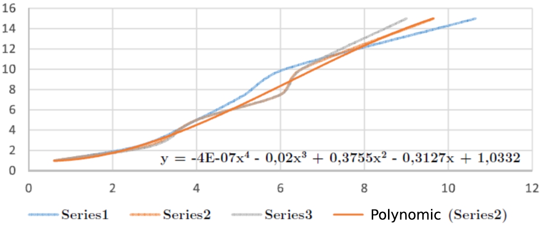
In Fig. 7 we plot the measurements of Table 2 as 3 curves (one for each column). Whilst the x-axis represents the measured distance by the application, the y-axis indicates the real distance between the beacon and the device. From these 3 series we generated a fourth-grade polynomial regression model. This model was used by the application to more accurately detect the distance between the guidance system and beacon
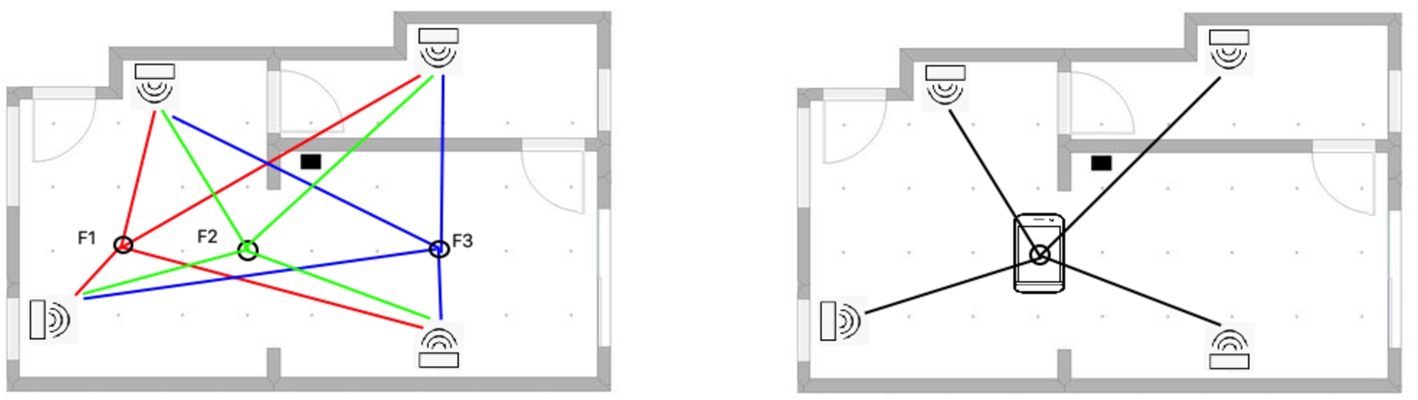
3.2.3.Comparative between map-based and MinMax location algorithms
In order to compare the two indoor location algorithms, we performed a visual analysis of the resulting trajectories with each approach. In that sense, given the ideal route of the use case depicted in Fig. 6, the combination of the MinMax algorithm and the calibration mechanism, produced the trajectory depicted in Fig. 8(a). Alternatively, the Map-Based algorithm generated the trajectory shown in Fig. 8(b). We can clearly see that this second trace is much more similar to the actual route followed by the visitor than the one obtained by the MinMax algorithm.
Table 3
Parameters settings for the FRCs generation
| Parameter | Involved step | Value |
| Trajectory segmentation | 1 m | |
| Trajectory segmentation | 5 m | |
| m | Trajectory clustering | 2.0 |
| ϵ | Trajectory clustering | 0.0001 |
Fig. 8.
Examples of two captured trajectories. The trace of each one is depicted as a black line. The BLE beacons are shown as small red squares.
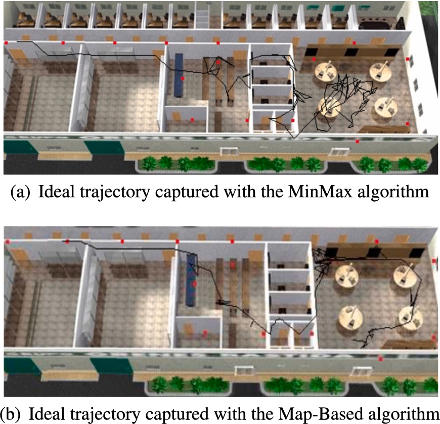
The main problem of the MinMax approach was that the distances that the BLE scanner library55 provided us were neither precise nor always repeatable. This made it rather difficult to accurately obtain the location of the devices. Therefore, the MinMax approach gave us poor results, even with the calibration refinement. On the contrary, our two-step Map-Based algorithm (described in Section 2.3.1) performed much better. This is because it does not rely on the measured distances to the beacons, but rather compare the measurements provided at any given time instant t with the ones stored in the previously-generated set
All in all, the MinMax algorithm achieved poorer results in terms of trajectory perception, because of the low reliability of the distances measured from the beacons. Even though we tried to tackle this problem with a calibration mechanism, we still did not achieve suitable results. Therefore, we eventually use our initial Map-based approach to capture the visitors’ movement actions for the rest of the use case analysis.
3.3.Trajectories classification
Once the indoor positioning system was calibrated, the FRCs for the collected trajectories were generated and tested.
3.3.1.Target classes
In the present setting, the goal of the classifier is to detect four types of visitors in the test-bed. In particular, the site operators come up with four different interesting behaviours. As a result, the target classes composing Ω are the following,
–
–
–
–
3.3.2.Collection of visitors’ trajectories
We collected 64 different trajectories during a 1-week period ranging from 19/04/17 to 25/04/17. Each one was manually labeled by the exhibition operators with one of the four classes previously mentioned. This gave rise to 16 trajectories of each class.
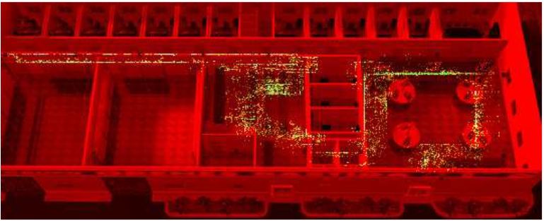
Figure 9 shows the heat map of every captured trajectories composing the
Fig. 9.
Heat map of all the collected trajectories. Pixels with color green have been more frequented by users, followed by yellow tones and finally in red we see unexplored places.
In Fig. 8, we can see two examples of collected trajectories. From these traces, we clearly observe the noisy and imprecise nature of such trajectories. This justifies the trajectory segmentation and feature extraction process to normalize the trajectories representation and the fuzzy logic approach to classify them.
3.3.3.Classifier configuration
Table 3 shows the key parameters used to generate the ensemble of FRCs. We can see that
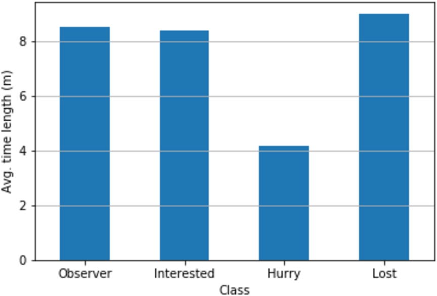
Fig. 10.
Average time length of trajectories in
3.3.4.Number of clusters per segment
In order to set the number of clusters
This way, we executed FCM multiple times with different numbers of clusters and calculated the FPC associated to each resulting partition keeping the one with the highest coefficient per segment number and class. Table 4 sums up the obtained number of clusters. For example, the suitable number of clusters for the second segment of trajectories with label
Table 4
Number of clusters per segment number and output class
| Class ( | Segment num. | Num. clusters ( |
| 1, 3, 4, 5, 7, 8, 10–15 | 1 | |
| 2 | 2 | |
| 6,9 | 3 | |
| 1–4, 8, 10–21 | 1 | |
| 9 | 2 | |
| 5-7 | 3 | |
| 2,5,6,7,8,9 | 1 | |
| 3,4 | 2 | |
| 1 | 3 | |
| 1,5 | 1 | |
| 2,4,6–21 | 2 | |
| 3 | 3 |
From this table we can see that most of the trajectory segments from observer, interested or hurry visitors could be aggregated into a single cluster. However, trajectories segments from lost visitors were mostly clustered in two clusters instead of one. This is compatible with the fact that this type of visitors tended to roam around the museum and thus, their movements were generally more diverse.
3.3.5.Classifier accuracy
Once the FRCs were generated on the basis of the aforementioned parameters, we studied its accuracy. For that goal, we used the F1 score as measurement. This score is calculated following the next formula:
Table 5 shows the recall, precision and F1 scores of RECITE. In order to evaluate the suitability of the segmentation approach, the table also shows the results of a FRC (
Table 5
Accuracy scores of the palette of FRCs of RECITE with and without velocity features and a monolithic FRC without including a trajectory segmentation step
| Model | Precision | Recall | F1 |
| RECITE FRCs | 0.95 | 0.94 | 0.94 |
| RECITE FRCs (+velocity feat.) | 0.92 | 0.93 | 0.92 |
| 0.84 | 0.79 | 0.79 |
From these results we can see that the trajectory segmentation step clearly helps to improve the classification accuracy. This is because RECITE generates a FRC for each possible sub-trajectory achieving a higher level of specialization and, thus, accuracy.
Furthermore, Table 6 shows the confusion matrix of the evaluation. In that sense, this matrix includes all the intermediate trajectories that users generate during their visits. In general, the main errors occur in adjacent labels. However, 4% of hurry sub-trajectories are classified as lost ones when these two labels are not very similar. In that sense, we have observed that, sometimes, some hurry visitors return to places already seen in their attempt to quickly cross the exhibition area. This makes such visitors mimic the behaviour of lost visitors.
Table 6
Confusion matrix of the RECITE FRCs. A cell in row R and column C with R ≠ C, contains the sheer number and percentage of sub-trajectories whose real label was R but it was wrongly classified as C
| Real | Inferred | |||
| Observer | Interested | Hurry | Lost | |
| Observer | 610 (89%) | 52 (7.6%) | 1 (0.1%) | 20 (2.9%) |
| Interested | 19 (2.8%) | 661 (97.2%) | 0 | 0 |
| Hurry | 0 | 0 | 415 (96.5%) | 15 (3.5%) |
| Lost | 25 (3.5%) | 33 (4.6%) | 0 | 659 (91.9%) |
The next aspect we evaluated was the impact of the length of an ongoing trajectory on the classifier. The results of this evaluation are shown in Fig. 11.
Fig. 11.
F1 score of the classifier per trajectory number of segments. Each bar depicts the F1 score of the FRCs for trajectories with number of segments equal to its x-axis value.
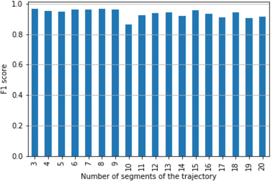
According to this figure, we can see the F1 score of the proposal was above 0.9 regardless of the number of segments of the target trajectory. However, the accuracy of our classifier was slightly higher for trajectories with segments ranging between 3 and 9. This was because this range of segments comprised most of the trajectories whereas the number of trajectories comprising more than 10 segments was much lower. This resulted in an accuracy drop of the solution.
3.4.New segment features sensitivity study
As it is put forward in Section 2.5, the present version of the framework extracts only three different features from each segment, namely the average x-y coordinates and the average number of content displays. Consequently, we also evaluated the effect in RECITE of adding new segment features as part of the framework, namely, the average segment speed and the average segment bearing.66 This way, we include the velocity of the trajectories so as to perceive in a more detailed manner the actual movement of the visitors in the museum.
Bearing in mind the definition 3, each trajectory segment feature
As Table 5 shows, including these features in the solution did not actually improve the accuracy of RECITE with respect to the baseline approach. This way, the F1 score was slightly lower (0.92 vs 0.94). Regarding the confusion matrix depicted in Table 7, we can see the velocity features slightly improved the detection of lost trajectories as their classification rate increased from 91.9% (see Table 6) to 93.7%. This type of trajectories are defined by many changes of direction due to the roaming behaviour of the visitors. As a result, the bearing features help to better identify these types of movements. Nevertheless, this rate actually dropped for the other three types of trajectories.
Table 7
Confusion matrix of the RECITE FRCs enriched with velocity features from the trajectories. A cell in row R and column C with R ≠ C, contains the sheer number and percentage of sub-trajectories whose real label was R but it was wrongly classified as C
| Real | Inferred | |||
| Observer | Interested | Hurry | Lost | |
| Observer | 598 (87.1%) | 76 (11.0%) | 5 (0.7%) | 7 (1.0%) |
| Interested | 27 (3.9%) | 667 (95.4%) | 5 (0.7%) | 0 |
| Hurry | 13 (3.4%) | 0 | 372 (96.6%) | 0 |
| Lost | 10 (1.4%) | 32 (4.3%) | 5 (0.7%) | 693 (93.7%) |
The reason of this lack of actual improvement of RECITE is due to the well-known curse of dimensionality problem [27]. Adding more features to the target input space makes the trajectories segments more distant among them. As a result, the approach generated much more clusters and, thus, fuzzy rules as we can see in the Table 8. According to this table, the system generated, for example, 8 different clusters given the first segments of the trajectories labelled as
Table 8
Number of clusters per segment number and output class with velocity features
| Class ( | Segment num. | Num. clusters ( |
| 3, 5, 6, 7, 9 | 3 | |
| 6 | 4 | |
| 2 | 5 | |
| 4 | 6 | |
| 1, 8 | 8 | |
| 1, 10-21 | 1 | |
| 4, 9 | 5 | |
| 2, 6, 7 | 6 | |
| 3, 8 | 7 | |
| 5 | 8 | |
| 6-9 | 1 | |
| 2, 3 | 5 | |
| 1, 5 | 6 | |
| 4 | 7 | |
| 9 | 1 | |
| 4, 7 | 3 | |
| 6 | 4 | |
| 3 | 5 | |
| 5, 8 | 6 | |
| 2 | 7 | |
| 1 | 8 |
Finally, FRCs are easily interpretable as they are composed of IF-THEN sentences. In this context, a drawback of enlarging the framework with new input features is that the complexity of the FRC increases and the aforementioned descriptive capability of this type of fuzzy systems is lost.
4.Related work
When it comes to deal with indoor trajectories in cultural spaces, it can be established three different characteristics to catalogue the existing literature: the type of enabling indoor positioning system, the modelling solution to represent the visitors movements and the type and purpose of the trajectory analysis over the collected data. Table 9 makes a review on each of these characteristics.
Table 9
Key features of existing indoor trajectory mining approaches in the cultural domain
| Ref. | Indoor Pos. System | Trajectory model | Trajectory analysis | ||
| Granularity | User interaction | Type(s) | Goal(s) | ||
| [32] | – BLE | Building element/POI | Audioguide events | – Trajectory clustering (k-Means) | Visiting patterns detection |
| [13] | – BLE | Coverage area | – | – Trajectory pattern mining (sequence alignment methods) | Visiting patterns detection |
| [23] | – RFID | POI | – | – Trajectory clustering (hierarchical clustering) – Trajectory pattern mining (frequent pattern mining) | Visiting patterns detection |
| [14] | – WiFi – Image recognition | Building elements | – | – Trajectory optimization ( | Museum indoor navigator |
| [22] | – RFID | POI | Visitor profile | – Trajectory classification (multi-layer perceptron, logistic regression) | Unseen POIs recommendation |
| [26] | – BLE | Building element | – | – Trajectory semantic enrichment | Visitors’ intention discovery |
| [39] | – BLE | Building element | – | – Trajectory pattern mining (frequency counting) | Visiting patterns detection |
| [38] | – BLE | Building element | – | – Trajectory pattern mining (random-walk model) | Visiting patterns detection |
| [12] | – BLE – Image recognition | POIs | – | – | – |
| [24] | – RFID | X-Y coordinates | – | – Trajectory clustering (k-Means) | Visiting patterns detection |
| [15] | – | Building element | – | – Stay-point Clustering | – Visitors’ behaviour timely detection |
| RECITE | – BLE | X-Y coordinates | Displayed content | – Trajectory clustering (FCM) – Trajectory classification | – Visiting patterns detection – Visitors’ behaviour timely detection |
4.1.Indoor positioning systems
To begin with, RFID readers have been widely used in this context so as to locate visitors holding different types of devices [41]. In that sense, approaches can be distinguished depending on the requirement of an explicit user check-in [22] or not [23,24].
Some works have also proposed WiFi access points as indoor positioning enablers. For example, [14] combines the signal strengths of WiFi routers and the outcome of an image-processing engine able to detect the presence of visitors to come up with a precise indoor positioning solution. Ambitrack [9] also proposed tracking through cameras and image-processing. However, this approach is more expensive to install and maintain than the inexpensive BLE beacons. An interesting approach to locate visitors in an art gallery is introduced in [12] where a combination of BLE beacons along with image recognition mechanism integrated in a wearable device allows to detect whether a visitor is in front of any art keypoint of a gallery. However, in most cases BLE is used to detect presence of visitors at much more large scale (e.g. galleries or corridors) [13,26,32,38,39].
Our work also makes use of an ad-hoc indoor positioning system relying on BLE. However, unlike other solutions we consider a careful calibration process performed at device and global level based on polynomial regression. Thus, we are able to accurately locate the visitor making use of affordable beacons as described in Section 2.3.
4.2.Trajectory modelling
Regarding a building-based approach, many solutions just perform a simple mapping step considering the concrete building space where the sensors is actually located to construct the visitors’ paths. Examples of this are [38,39] that model trajectories as sequences of visited galleries. However, [15] relies on a museum graph model that accurately represents its premises, like doors, rooms or vitrines. Then, a mapping approach is performed to convert the collected spatio-temporal data from users to the graph-based representation. However, the proposal does not define any particular indoor positioning system to capture the visitors’ movement. A similar approach is followed by [1,26] where a semantic indoor trajectory model is proposed or [14] with a more holistic ontology.
POI-based approaches have also been widely used in the literature [12,22,23]. In some cases, this type of models are enriched with additional information. For example, [22] merges the visited POIs along with the digital content consulted by the user in the museum displays to compose the set of features that defines the user’s movement.
Furthermore, it is interesting to mention the work in [13] where the building bricks to compose user trajectories are the named coverage areas of the Bluetooth beacons. Thus, it provides an intermediate solution between POIs and building elements to represent the visitors’ trajectories. Similarly, [32] considers both POIs (artworks) and building elements (rooms) to compose the trajectories.
Our work is enclosed on an alternative way to model trajectories based on a two-dimensional Cartesian space. In this domain, only a few works have actually relied on this representation. For instance, [24] makes use of this technology to calculate the probability of a visitor’s position in a map image representing a gallery floor. The RECITE model leverages the accuracy of the underlying positioning system. As a result, we have been able to perform certain computations from the outdoor trajectory mining field like the segmentation step discussed in Section 2.4. Moreover, our work enriches this model by labelling certain segments of the trajectory with the content displayed by the user in his guidance device.
4.3.Trajectory analysis
Concerning the analysis of the collected trajectories, there is a wide range of solutions considering both the applied methods and their purpose. To begin with, some examples can be found where trajectory pattern mining has been carried out by means of simple frequency counting methods to discover the most frequent sequences of visited galleries [39]. In [13], authors pursue the same goal but, in this case, sequence alignment methods are applied over trajectory data. In [38] trajectories are characterized using the random walk model.
As far as trajectory clustering is concerned, many different algorithms has been tested. For instance, [24,32] make use of the k-Means clustering algorithm to aggregate visitors’ trajectories and, thus, uncover general movement trends. However, [24] performs a spatial partitioning by means of the state chain model before applying the clustering algorithm. In [23], authors perform a clustering task over the set of trajectories and map each cluster to a set of predefined visitor profiles. Later on, two sequence miners are applied to each group in order to reveal interesting patterns defining visitor behaviors.
Other works have used optimization algorithms like
In addition to that, some works just provide a preliminary design of the trajectory analysis that might be carried out. For example, [15] proposes to identify stay-points of visitors’ routes and then performs an incremental clustering over such points using time windows to detect behaviour changes during consecutive time intervals. Another worth mentioning work is [26]. It provides a semantic reasoning mechanism that, by means of a set of domain-dependent predicates, it is able to infer the purpose of visitors’ movements (e.g. visit a particular gallery or buy something at the gift shop).
In the trajectory classification field, we have noticed a scarcity of proposals within the cultural domain. Thus, [22] makes use of two well-established classification algorithms like logistic regression and multi-layer perceptron to rate the suitability of an unseen POI recommendation based on the previous movement of a user. For that goal, some profiling information of the visitor like age or gender is considered.
In this context, the work at hand provides a set of FRCs that smoothly merges the spatio-temporal data from visitors displacements and data related to the content displayed in the guidance devices to timely detect the visitors behaviour. To do so, it does not rely on any sensitive profiling data from users.
We should also mention that our work share some similarities with the proposal stated in [11]. In that work, a FRC-based mechanism to classify trajectories based on Volunteer Geographic Information (VGI) is described. However, VGI provides a more coarse-grained representation of the target users’ movement than in our setting. Consequently, a segmentation step is not necessary in that work. Furthermore, in such a work, only the spatio-temporal features of the trajectories are considered for the classification task whereas RECITE also considers other factors like the usage of the multimedia content made by visitors.
5.Conclusions
The cultural domain is endlessly taking advantage of IoT-related technologies. This has generated a huge amount of visitors’ data so as to come up with innovative services in museums and exhibition areas.
In this context, the present work introduces the RECITE framework. On the basis of a BLE infrastructure acting as an indoor positioning system, this framework is able to detect the movement of visitors in a cultural site and track the usage they make of the multimedia content available at their guidance devices.
On top of the collected indoor trajectory data, an ensemble of fuzzy rules classifiers is developed. Such classifiers are able to tag in real time the behaviour of visitors based on their movements and their usage of the multimedia content. To do so, we have followed a data-driven methodology that combines algorithms and techniques from different fields. To begin with, a segmentation method from the trajectory data mining field has been included so as to provide an uniform representation of the heterogeneous trajectories. Secondly, the fuzzy clustering algorithm FCM has been applied to uncover similarities in the movement behaviour of visitors and eventually compose the final fuzzy rules classifiers.
Finally, we have evaluated the framework in a test-bed scenario. In that setting, we have compared two different approaches to provide an indoor positioning system using BLE as enabling technology. The comparison shown that the mechanism based on a pre-defined map of locations provide a more accurate solution in terms of trajectory perception. Regarding the classification features of RECITE, results showed that the FRC approach allowed to accurately classify visitors as they move around the site and access the multimedia data provided by the museum.
Notes
6 In the present setting, a trajectory’s segment bearing is regarded as the clockwise angle in degrees between north and the segment’s vector.
Acknowledgements
This work has been supported by the Fundación Séneca del Centro de Coordinación de la Investigación de la Región de Murcia under Project 20813/PI/18, by the Spanish Ministry of Science, Innovation and Universities under grant RTC-2017-6389-5, by the PERSEIDES project TIN2017-86885-R and also co-financed with ERDF funds.
Conflict of interest
The authors have no conflict of interest to report.
References
[1] | I. Afyouni, S. Ilarri, C. Ray and C. Claramunt, Context-aware modelling of continuous location-dependent queries in indoor environments, Journal of Ambient Intelligence and Smart Environments 5: (1) ((2013) ), 65–88. doi:10.3233/AIS-120186. |
[2] | S. Alletto, R. Cucchiara, G. Del Fiore, L. Mainetti, V. Mighali, L. Patrono and G. Serra, An indoor location-aware system for an IoT-based smart museum, IEEE Internet of Things Journal 3: (2) ((2016) ), 244–253. doi:10.1109/JIOT.2015.2506258. |
[3] | B. Alsinglawi, M. Elkhodr, Q.V. Nguyen, U. Gunawardana, A. Maeder and S. Simoff, RFID localisation for Internet of Things smart homes: A survey, 2017, preprint arXiv:1702.02311. |
[4] | F. Arcas-Tunez and F. Terroso-Saenz, Forest path condition monitoring based on crowd-based trajectory data analysis, Journal of Ambient Intelligence and Smart Environments 13: (1) ((2021) ), 24–54. doi:10.3233/AIS-200586. |
[5] | R. Babus˘ka, Fuzzy Modeling and Identification, International Series in Intelligent Technologies, Kluwer Academic Publishers, (1998) . |
[6] | A. Basiri, E.S. Lohan, T. Moore, A. Winstanley, P. Peltola, C. Hill, P. Amirian and P.F. e Silva, Indoor location based services challenges, requirements and usability of current solutions, Computer Science Review 24: ((2017) ), 1–12, http://www.sciencedirect.com/science/article/pii/S1574013716301782. doi:10.1016/j.cosrev.2017.03.002. |
[7] | J.C. Bezdek, Pattern Recognition with Fuzzy Objective Function Algorithms, Springer Science & Business Media, (2013) . |
[8] | J.C. Bezdek, R. Ehrlich and W. Full, FCM: The fuzzy c-means clustering algorithm, Computers and Geosciences 10: (2) ((1984) ), 191–203, http://www.sciencedirect.com/science/article/pii/0098300484900207. doi:10.1016/0098-3004(84)90020-7. |
[9] | A. Braun and T. Dutz, Low-cost indoor localization using cameras–evaluating ambitrack and its applications in ambient assisted living, Journal of Ambient Intelligence and Smart Environments 8: (3) ((2016) ), 243–258. doi:10.3233/AIS-160377. |
[10] | R.F. Brena, J.P. García-Vázquez, C.E. Galván-Tejada, D. Muñoz-Rodriguez, C. Vargas-Rosales and J. Fangmeyer, Evolution of indoor positioning technologies: A survey, Journal of Sensors 2017 (2017). |
[11] | J. Cuenca-Jara, F. Terroso-Sáenz, M. Valdés-Vela and A.F. Skarmeta, Classification of spatio-temporal trajectories from volunteer geographic information through fuzzy rules, Applied Soft Computing 86: ((2020) ), 105916, http://www.sciencedirect.com/science/article/pii/S1568494619306970. doi:10.1016/j.asoc.2019.105916. |
[12] | G. Del Fiore, L. Mainetti, V. Mighali, L. Patrono, S. Alletto, R. Cucchiara and G. Serra, A location-aware architecture for an IoT-based smart museum, International Journal of Electronic Government Research (IJEGR) 12: (2) ((2016) ), 39–55. doi:10.4018/IJEGR.2016040103. |
[13] | M. Delafontaine, M. Versichele, T. Neutens and N. Van de Weghe, Analysing spatiotemporal sequences in bluetooth tracking data, Applied Geography 34: ((2012) ), 659–668, http://www.sciencedirect.com/science/article/pii/S014362281200029X. doi:10.1016/j.apgeog.2012.04.003. |
[14] | J. Duque Domingo, C. Cerrada, E. Valero and J.A. Cerrada, A semantic approach to enrich user experience in museums through indoor positioning, in: Ubiquitous Computing and Ambient Intelligence, S.F. Ochoa, P. Singh and J. Bravo, eds, Springer International Publishing, Cham, (2017) , pp. 612–623. ISBN 978-3-319-67585-5. doi:10.1007/978-3-319-67585-5_60. |
[15] | G. Elmamooz, B. Finzel and D. Nicklas, Towards understanding mobility in museums, in: Datenbanksysteme für Business, Technologie und Web (BTW 2017) – Workshopband, B. Mitschang, D. Nicklas, F. Leymann, H. Schöning, M. Herschel, J. Teubner, T. Härder, O. Kopp and M. Wieland, eds, Gesellschaft für Informatik e.V., Bonn, (2017) , pp. 127–136. |
[16] | M.R. Emami, I.B. Turksen and A.A. Goldenberg, Development of a systematic methodology of fuzzy logic modeling, Fuzzy Systems, IEEE Transactions on 6: (3) ((1998) ), 346–361. doi:10.1109/91.705501. |
[17] | R. Faragher and R. Harle, Location fingerprinting with bluetooth low energy beacons, IEEE Journal on Selected Areas in Communications 33: (11) ((2015) ), 2418–2428. doi:10.1109/JSAC.2015.2430281. |
[18] | N. Fet, M. Handte and P.J. Marrón, Autonomous adaptation of indoor localization systems in smart environments, Journal of Ambient Intelligence and Smart Environments 9: (1) ((2017) ), 7–20. doi:10.3233/AIS-160416. |
[19] | M. Gams, I.Y.-H. Gu, A. Härmä, A. Muñoz and V. Tam, Artificial intelligence and ambient intelligence, Journal of Ambient Intelligence and Smart Environments 11: (1) ((2019) ), 71–86. doi:10.3233/AIS-180508. |
[20] | A.F. Gómez-Skarmeta, M. Delgado and M.A. Vila, About the use of fuzzy clustering techniques for fuzzy model identification, Fuzzy Sets and Systems 106: (2) ((1999) ), 179–188, http://www.sciencedirect.com/science/article/pii/S0165011497002765. doi:10.1016/S0165-0114(97)00276-5. |
[21] | M. Gribaudo, M. Iacono and A.H. Levis, An IoT-based monitoring approach for cultural heritage sites: The matera case, Concurrency and Computation: Practice and Experience 29: (11) ((2017) ), e4153. doi:10.1002/cpe.4153. |
[22] | S.H. Hashemi and J. Kamps, Exploiting behavioral user models for point of interest recommendation in smart museums, New Review of Hypermedia and Multimedia 24: (3) ((2018) ), 228–261. doi:10.1080/13614568.2018.1525436. |
[23] | N. Juniarta, M. Couceiro, A. Napoli and C. Raïssi, Sequential pattern mining using FCA and pattern structures for analyzing visitor trajectories in a museum, in: CLA 2018 – the 14th International Conference on Concept Lattices and Their Applications, Olomouc, Czech Republic, (2018) , https://hal.inria.fr/hal-01887914. |
[24] | T. Kanda, M. Shiomi, L. Perrin, T. Nomura, H. Ishiguro and N. Hagita, Analysis of people trajectories with ubiquitous sensors in a science museum, in: Proceedings 2007 IEEE International Conference on Robotics and Automation, (2007) , pp. 4846–4853, ISSN 1050-4729. doi:10.1109/ROBOT.2007.364226. |
[25] | A. Kontarinis, C. Marinica, D. Vodislav, K. Zeitouni, A. Krebs and D. Kotzinos, Towards a better understanding of museum visitors’ behavior through indoor trajectory analysis, in: Seventh International Conference on Digital Presentation and Preservation of Cultural and Scientific Heritage (DiPP2017), Vol. 7: , (2017) , pp. 19–30. |
[26] | A. Kontarinis, K. Zeitouni, C. Marinica, D. Vodislav and D. Kotzinos, Towards a semantic indoor trajectory model, in: EDBT/ICDT Workshops, (2019) . |
[27] | M. Köppen, The curse of dimensionality, in: 5th Online World Conference on Soft Computing in Industrial Applications (WSC5), Vol. 1: , (2000) , pp. 4–8. |
[28] | D. Kosmopoulos and G. Styliaras, A survey on developing personalized content services in museums, Pervasive and Mobile Computing 47: ((2018) ), 54–77, http://www.sciencedirect.com/science/article/pii/S1574119217305138. doi:10.1016/j.pmcj.2018.05.002. |
[29] | V.D. Ambeth Kumar, G. Saranya, D. Elangovan, V.R. Chiranjeevi and V.D. Ashok Kumar, IOT-based smart museum using wearable device, in: International Conference on Innovative Computing and Communications, S. Bhattacharyya, A.E. Hassanien, D. Gupta, A. Khanna and I. Pan, eds, Springer, Singapore, (2019) , pp. 33–42. ISBN 978-981-13-2324-9. doi:10.1007/978-981-13-2324-9_5. |
[30] | J. Paek, J. Ko and H. Shin, A measurement study of BLE iBeacon and geometric adjustment scheme for indoor location-based mobile applications mobile information systems, Mobile Information Systems 2016: ((2016) ), 8367638. doi:10.1155/2016/8367638. |
[31] | N.R. Pal, J.C. Bezdek and E.-C. Tsao, Generalized clustering networks and Kohonen’s self-organizing scheme, IEEE Transactions on Neural Networks 4: (4) ((1993) ), 549–557. doi:10.1109/72.238310. |
[32] | F. Piccialli, Y. Yoshimura, P. Benedusi, C. Ratti and S. Cuomo, Lessons learned from longitudinal modeling of mobile-equipped visitors in a complex museum, Neural Computing and Applications ((2019) ). doi:10.1007/s00521-019-04099-8. |
[33] | J. Rada-Vilela, The FuzzyLite Libraries for Fuzzy Logic Control, 2018, https://fuzzylite.com/. |
[34] | M. Radhakrishnan, A. Misra, R.K. Balan and Y. Lee, Smartphones and BLE services: Empirical insights, in: 2015 IEEE 12th International Conference on Mobile Ad Hoc and Sensor Systems, (2015) , pp. 226–234. doi:10.1109/MASS.2015.92. |
[35] | N. Streitz, D. Charitos, M. Kaptein and M. Böhlen, Grand challenges for ambient intelligence and implications for design contexts and smart societies, Journal of Ambient Intelligence and Smart Environments 11: (1) ((2019) ), 87–107. doi:10.3233/AIS-180507. |
[36] | T. Takagi and M. Sugeno, Fuzzy identication of systems and its application to modeling and control, IEEE Trans. Systems, Man, and Cybernet 15: ((1985) ), 116–132. doi:10.1109/TSMC.1985.6313399. |
[37] | S. Xia, Y. Liu, G. Yuan, M. Zhu and Z. Wang, Indoor fingerprint positioning based on Wi-Fi: An overview, ISPRS International Journal of Geo-Information 6: (5) ((2017) ), 135. doi:10.3390/ijgi6050135. |
[38] | Y. Yoshimura, R. Sinatra, A. Krebs and C. Ratti, Analysis of visitors’ mobility patterns through random walk in the Louvre museum, 2018, preprint arXiv:1811.02918. |
[39] | Y. Yoshimura, S. Sobolevsky, C. Ratti, F. Girardin, J.P. Carrascal, J. Blat and R. Sinatra, An analysis of visitors’ behavior in the Louvre museum: A study using bluetooth data, Environment and Planning B: Planning and Design 41: (6) ((2014) ), 1113–1131. doi:10.1068/b130047p. |
[40] | L.A. Zadeh, The concept of a linguistic variable and its application to approximate reasoning – I, Information Sciences 8: (3) ((1975) ), 199–249, http://www.sciencedirect.com/science/article/pii/0020025575900365. doi:10.1016/0020-0255(75)90036-5. |
[41] | L. Zamora-Cadenas, A. Cortés and I. Vélez, Radiofrequency-based indoor location systems for ambient assisted living applications, Journal of Ambient Intelligence and Smart Environments 6: (5) ((2014) ), 561–563. doi:10.3233/AIS-140278. |
[42] | Y. Zheng, Trajectory data mining: An overview, ACM Trans. Intell. Syst. Technol. 6: (3) ((2015) ), 29:1–29:41. doi:10.1145/2743025. |


