
Assessment and clustering of temporal disaster risk: Two case studies of China
Abstract
Disaster risk assessment is the foundation to carry out a comprehensive disaster reduction. Despite a growing body of literature on this subject, dynamic risk assessment concerning the temporal characteristic of disaster risk receives relatively inadequate attention in previous research. This paper focuses on analyzing the temporal disaster risk over a period to enable decision makers to understand the risk variation explicitly and hence take long-term countermeasures for improving the prevention and mitigation of hazards. It is achieved by firstly evaluating the risk temporally and then aggregating the alternatives through a hybrid clustering method based on the similarity between risk vectors. The proposed method is employed to two case studies of China concerning public health events and natural disasters respectively. The risk variation disclosed brings insight into the properties of investigated alternatives and therefore contributes to effective disaster reduction.
1.Introduction
Disaster is the sudden happened event, which may cause serious harm to human being, society and economy. It can be categorized in different perspectives. According to the generation, characteristics and forming mechanism, disasters are divided into four groups, namely natural disasters, accidental disasters, public health events and social security events. Natural disasters refer to the casualties, property loss and resource damage caused by natural mutation, including meteorological disasters, geological disasters, marine disasters, forest fires, biological disasters, etc. Accident disasters mostly caused by man-made production and living activities include traffic accidents, safety accidents, urban lifeline accidents, etc. Social security incidents refer to the events that endanger the normal social order and undermine the social stability. Public health events include infectious diseases, unknown causes diseases, major food and occupational poisoning, etc. Nowadays the pandemic Coronavirus Disease-2019 (COVID-19) is having a formidable impact on people and societies all over the world since the first reported case in 2019. Despite the remarkable progress on vaccine development, the negative impact brought by COVID-19 will continue and even escalate for a long time.
Decision making is the process of selecting a possible solution from all available alternatives or ranking the alternatives into preference-ordered classes according to a predefined evaluation measurement. Risk assessment is essential across many industries to determine the likelihood of loss. It is usually solved as single-objective decision making (SODM) or multi-criteria decision making (MCDM) depended on the complexity of problem. Single objective decision making which aims to meet the requirements of certain objective is commonly solved by break-even point analysis, critical cost method, differential analysis method, linear programming, nonlinear programming, dynamic programming, evolutionary programming, etc [4, 28]. Multi-criteria decision making concerns multiple objectives that are usually complicated or even conflicting. The traditionally used approaches include TOPSIS (Technique for Order Preference by Similarity to Ideal Solution), VIKOR (VIsekriterijumska optimizacija i KOmpromisno Resenje), AIRM (Aggregated Indices Randomization Method), AHP (Analytic Hierarchy Process), ANP (Analytic Network Process), BWM (Best Worst Method), DEA (Data Envelopment Analysis), DEMATEL (Decision Making Trial and Evaluation Laboratory), DEX (Decision EXpert), ER (Evidential Reasoning), GP (Goal Programming), GRA (Grey Relational Analysis), IPV (Inner Product of Vectors), Rough Set etc [10, 14, 26]. Recently advanced computational intelligence approaches such as artificial neural network, support vector machine, genetic algorithm, fuzzy cognitive maps have gained considerable attention in multi-criteria decision making problems [13, 25, 31].
In emergency management, disaster risk assessment is a process to evaluate the probability and degree of potential hazards, and analyze what could happen if a hazard occurs. Despite the diversity of hazards, risk assessment is considered as a vital task for improving the prevention and mitigation capability of the affected body as well as reducing the harm caused by hazards through effective emergency management countermeasures.
There is much evidence that the temporal characteristic of data are more and more concerned recently. Camacho-Munoz et al. studied the temporal evolution of pharmaceuticals in the main river affecting Donana Park (Spain) during one year [6]. Zhao et al. considered the spatial and temporal variations in a long-term forewarning model of flood disaster for Tunxi area, Huangshan City of China using a back-propagation neural network [34]. A dynamic risk assessment of drought disaster was developed to maize production in the northwest of Liaoning Province based on remote sensing data [24]. A methodology was proposed for risk assessment of drought disaster using real-time precipitation and multi-source remote sensing data [17]. Bach et al. employed a dynamic and probability based methodology called catastrophe simulation model to evaluate the present and future disaster risk [5]. Chen et al. adopted fuzzy matter element theory to analyse the contributing factors of world total-loss marine casualty and discuss the different influence of these factors to the evolution trend of total losses [8]. In brief, the previous studies concerned either temporal risk of a single object or static risk of multiple objects [12, 27], however contained few attempt to risk variation analysis of diverse objects.
This study is intended to analyze the variation of disaster risk by temporal risk assessment and clustering. The risk assessment is first performed temporally to generate a risk vector for each alternative. Afterwards a clustering process is employed based on the similarity between risk vectors measured by a distance metric. The proposed approach is applied to two case studies of China concerning public health events and natural disasters respectively. In the former, the occurrence of 26 infectious diseases was monitored in Zhengzhou, the capital of Henan province, from May 2014 to March 2019. The risk of diseases is proportional to the frequency of occurrence. The clusters of temporal risk found reveal the seasonality and co-occurrence property of infectious diseases. In the latter, the statistical data of 31 Chinese regions to natural disasters was collected from 2014 to 2018. After yearly evaluating the regional risk defined as the risk of regions to natural disasters, the regions are grouped to several clusters characterized by risk variation. Different from the existing studies that usually focus on trend detection of a single disaster event, we provide a novel perspective on risk variation analysis and clustering. The paper enriches the analysis of temporal disaster risk by characterizing the variation of risk over the entire distribution. The findings provide an improved understanding of the variation of disaster risk and therefore have significant importance to enhance the effectiveness of countermeasures to disaster reduction. Although the case study did not include COVID-19 due to the data acquisition problem, the proposed method could be applied to the issue for analyzing the risk variation across different countries (regions) and infectious diseases.
The rest of this paper is organized as follows. Section 2 outlines the methodology of risk assessment and variation analysis for temporal data. Section 3 is devoted to some analytic results of two case studies using the proposed approach. Finally, section 4 concludes the paper along with some suggestions and highlights the future directions.
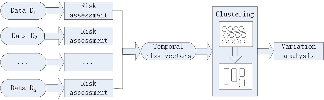
Figure 1.
Framework of dynamic risk assessment and variation analysis.
2.Methodology and framework of research
In this section we introduce an approach for temporal risk assessment and variation analysis. Figure 1 schematically describes the framework of the proposed approach. The input is a temporal data set {
Clustering as an unsupervised learning task by nature divides the unlabeled data set into a number of groups that maximize the intra-similarity and minimize the inter-similarity. By definition, the former indicates the similarities within groups and the latter indicates the similarities across groups.
SOM [20] is a kind of neural network used for unsupervised learning. It is composed of input neurons and output neurons that set along a grid. Input neurons are served as feeding the input data, and output neurons adjust the spatial structure gradually in order to recognize the distribution of input data. Each output neuron is associated with a codebook vector which represents a cluster of input. For each input SOM finds a neuron to which best matches, called best-matching unit (BMU). Then the codebook vector of BMU is updated by the random gradient descent. Meantime the adjacent neurons update the codebook vectors according to their distance from BMU. Consequently the neurons are topologically ordered on the grid gradually in such manner that if instances are similar in the input space, then they will be likely projected to the same or nearby neurons in the map grid space. SOM has some promising merits, for example, clustering high dimensional data, preserving the topological properties, and visualizing cluster structures in an easily understandable manner. SOM has been widely applied as a standard analytical tool in a wide range of applications, including fault diagnosis, crop evapotranspiration, clinical voice analysis, satellite images analysis, landslide susceptibility, motorcycle hazard detection and so forth [1, 18, 23].
Let
(1) For
A neighborhood kernel function
After training each neuron corresponds to a cluster so that the input data is grouped to a number of clusters with respect to BMU. Although SOM facilitates the visualization and property exploration of data, it suffers from some drawbacks. For instances, it requires the user to specify the number of clusters. It is also difficult to find obvious clustering boundaries in the SOM results even with the easily understandable manner such as u-matrix (unified distance matrix) for visualizing cluster structures. To address these problems the hybrization of SOM and K-means proposed by [30] was found to perform well in market segmentation [21], classifying sensor data [22], identifying dynamic of biogeochemical properties [29], categorizing gene expression data [32], etc. In this study, the hybrid approach is employed to cluster the risk vectors. In specific the input is divided into a number of small and compact groups with respect to SOM neurons, and then aggregated to a few clusters using K-means.
K-means aims to divide a set of objects
3.Case studies: Results and discussions
In this section, the proposed method is utilized in two case studies of China. One is the risk of infectious diseases in Zhengzhou City, the other is the regional risk to natural disasters of China. Both data sets are temporal, however the latter is more complicated due to the multiple criteria involved in risk assessment.
3.1Risk of infectious diseases in Zhengzhou
Infectious disease can spread widely among people or between people and animals. It can be transmitted through air, water, food, soil, vertical transmission and direct contact with infected individuals, body fluids and excreta of infected persons, and objects contaminated by patients. According to the transmission mode, infectious diseases include: (1) respiratory infectious diseases (e.g., influenza, tuberculosis, mumps, measles, pertussis) commonly infected by air borne; (2) digestive tract infectious diseases (e.g., ascariasis, bacillary dysentery, hepatitis A) commonly infected by water and food; (3) blood infectious diseases (e.g., hepatitis B, malaria, epidemic encephalitis B, filariasis) mostly spread through biological media; (4) surface infectious diseases (e.g., schistosomiasis, trachoma, rabies, tetanus) characterized by contact transmission; (5) sexually transmitted diseases (e.g., gonorrhea, syphilis, AIDS). According to the speed and degree of harm to human beings as well as the measures of supervision, monitoring and management, infectious diseases are divided into three classes in China, i.e., compulsorily managed infectious diseases (Class A), strictly managed infectious diseases (Class B), supervisory infectious diseases (Class C). The first class including plague and cholera should be compulsively managed from the occurrence of diseases, then the isolation and treatment of patients and pathogen carriers, to the treatment of epidemic spots and epidemic areas. The second class including 26 infectious diseases should be prevented and controlled in strict accordance with the relevant regulations and prevention plans. The third class includes influenza, mumps, rubella, acute hemorrhagic conjunctivitis, leprosy, epidemic and endemic typhus, Kala Azar, hydatidosis, filariasis, infectious diarrhea, hand-foot-mouth disease, bacterial and amoebic dysentery, typhoid and paratyphoid.
Zhengzhou, the capital of Henan province, is an important megacity of more than 10 million population in Central China. Referring to the international unified classification standards and the actual situation of Zhengzhou, 26 kinds of acute and chronic infectious diseases listed in Table 1 with high incidence, wide epidemic area and serious harm are concerned in the case study. The occurrence of these infectious diseases was monitored during the period from May 2014 to March 2019 (46 months totally) except some unavailable data. Characterized by single objective of the problem, the risk caused by infectious diseases to the city is simply measured by the occurrence frequency of diseases. Quite evidently the more the value of occurrence, the more the risk of the infectious disease. The absolute frequency values are therefore normalized to [0, 1] where 1 indicates the highest risk and 0 indicates the lowest risk. After risk assessment the data is transformed to a matrix of
Table 1
Infectious diseases concerned in the first case study
| No. | Infectious disease | Transmission mode | Class |
|---|---|---|---|
| 1 | AIDS | Sexually transmitted diseases | B |
| 2 | HIV | Sexually transmitted diseases | B |
| 3 | Hepatitis A | Digestive tract infectious diseases | B |
| 4 | Hepatitis B | Blood infectious diseases | B |
| 5 | Hcv | Blood infectious diseases | B |
| 6 | Hev | Digestive tract infectious diseases | B |
| 7 | Measles | Respiratory infectious diseases | B |
| 8 | Hemorrhagic fever | Respiratory/Digestive tract/Surface infectious diseases | B |
| 9 | Rabies | Surface infectious diseases | B |
| 10 | Dengue fever | Blood infectious diseases | B |
| 11 | Dysentery | Digestive tract infectious diseases | B |
| 12 | Pulmonary tuberculosis | Respiratory infectious diseases | B |
| 13 | Typhoid | Digestive tract infectious diseases | B |
| 14 | Cerebrospinal meningitis | Blood infectious diseases | B |
| 15 | Pertussis | Respiratory infectious diseases | B |
| 16 | Scarlet fever | Respiratory infectious diseases | B |
| 17 | Brucellosis | Surface infectious diseases: | B |
| 18 | Gonorrhea | Sexually transmitted diseases | B |
| 19 | Syphilis | Sexually transmitted diseases | B |
| 20 | Malaria | Blood infectious diseases | B |
| 21 | Influenza | Respiratory infectious diseases | C |
| 22 | Mumps epidemic | Respiratory infectious diseases | C |
| 23 | Rubella | Respiratory infectious diseases | C |
| 24 | Acute hemorrhagic conjunctivitis | Surface infectious diseases | C |
| 25 | Other infectious diarrhea | Digestive tract infectious diseases | C |
| 26 | Hand-foot-mouth disease | Respiratory/Digestive tract/Surface infectious diseases | C |
Table 2
Five clusters of infectious diseases in terms of risk
| Cluster | Infectious diseases |
|---|---|
| #1 | AIDS, HIV, Hepatitis-A, Hev, Measles, Hemorrhagic fever, Rabies, Dengue fever, Dysentery, Typhoid |
| Cerebrospinal meningitis, Pertussis, Scarlet fever, Brucellosis, Gonorrhea, Malaria, Rubella, Acute hemorrhagic conjunctivitis | |
| #2 | Influenza |
| #3 | Hand-foot-mouth disease |
| #4 | Hepatitis B, Other infectious diarrhea |
| #5 | Hcv, Pulmonary tuberculosis, Syphilis, Mumps epidemic |
Figure 2.
SOM representation of infectious diseases by (a) u-matrix, (b) labels.
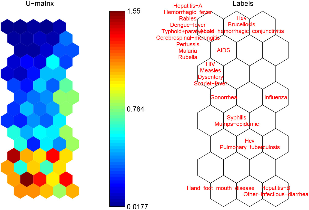
Figure 3.
Parallel coordinate visualization of infectious diseases for each cluster.
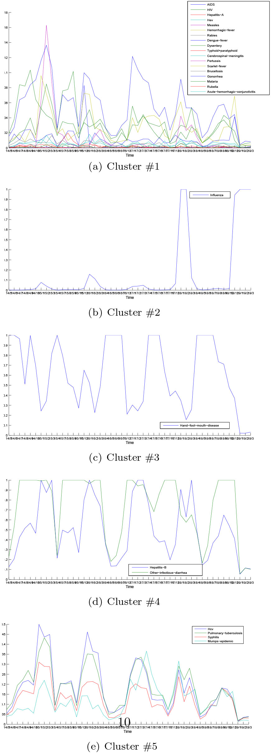
The generated risk vectors are fed to a SOM model for clustering. Figure 2 shows the u-matrix (a) and labels (b) projected to each neuron after SOM training. U-matrix visualizes the distances between the adjacent neurons with different colorings so that the insight of the data distribution can be observed without priori information about the clusters. In specific, a red coloring corresponds to a large distance and thus a gap between the codebook values in the input space. On the contrary, a blue coloring corresponding to a small distance signifies that the codebook vectors are close to each other in the input space. In this manner blue areas can be thought as clusters separated by red areas. After training each disease is assigned to the neuron whose codebook vector is most similar. The corresponding label of diseases are shown in the place of the neuron. The u-matrix representation in Fig. 2a reveals that the neurons in the upper left corner are close to each other, but differ from those in the bottom. Referring to the labels in Fig. 2b, the distribution of investigated infectious diseases can be grasped roughly in a straight way. In general, the diseases in the upper of SOM constitute a separated cluster and those in the bottom belong to several clusters respectively. In the following, K-means is used to find the cluster structure on the basis of the codebook vectors of SOM. The optimal cluster number is determined by DB index. The resulted five clusters are listed in Table 2. Accordingly the parallel coordinate visualization of infectious diseases with respect to each cluster is given in Fig. 3 where the x-axis denotes the time (formatted as year/month), and the y-axis denotes the risk (calculated as normalized occurrence frequency) of diseases. The 18 infectious diseases located in Cluster #1 remain a low level risk (less than 0.15 mostly) during the period despite some small fluctuations. The other 8 diseases occur more frequently characterized by the obvious seasonality but with different properties. Both Cluster #2 and Cluster #3 include one disease, namely Influenza and Hand-foot-month disease respectively. The corresponding parallel coordinate reveals that Influenza usually breaks out in winter and spring called as flu season. Particularly people infected by Influenza in 2017 and 2018 are significantly more than the same period of previous years likely due to the high air pollution [15]. It broke out since November and gradually entered a high incidence period until Match of the next year. Hand-foot-mouth disease caused by enterovirus mostly occurs in children under 5 years old. It can cause herpes in hands, feet, mouth and other parts even along with complications such as myocarditis, pulmonary edema, aseptic meningoencephalitis. In China the disease was first found in Shanghai in 1981, and has been reported in many regions so far. The occurrence frequency of Hand-foot-month disease varies dramatically during the whole year, and it usually breaks out and transmits rapidly in spring and summer. Cluster #4 includes Hepatitis B and other infectious diarrhea, which reach the peak for the incidence and infection in winter. Among Chinese legal infectious diseases, the incidence of Hepatitis B virus infection is reported very high only next to epidemic influenza and diarrhea. Cluster #5 comprises Hcv, Pulmonary tuberculosis, Syphilis and Mumps epidemic which usually break out in winter, spring and summer. As a high incidence area of tuberculosis and hepatitis virus, the patients infected by both Pulmonary tuberculosis and Hepatitis C virus are clinically common. The co-occurrence of Hcv and Pulmonary tuberculosis is distinctly presented in the parallel coordinate visualization of the two diseases.
Table 3
Evaluation index system of Chinese regional risk to natural disasters (
| Harm | Number of death (person) | ||
| Number of people affected by natural disasters (ten thousand) | |||
| Direct economic losses (100 million yuan) | |||
| Area of damaged crops (thousand hectare) | |||
| Vulnerability | Sensitivity | Regional population (ten thousand) | |
| Proportion of rural and urban population | |||
| Urban population density (person/km | |||
| Cultivated land (thousand hectare) | |||
| Building density | |||
| Response Ability | Number of medical & technical personnel per ten thousand residence | ||
| Number of medical beds per ten thousand people | |||
| Original property insurance revenue | |||
| Number of medical institutions | |||
| Budget expenditure for disasters | |||
| Number of seismic stations | |||
| Number of automatic meteorological station | |||
| Adaptability | Water amount per capita | ||
| Sex ratio (per 100 female) | |||
| Elderly population ratio (per 100 adults) | |||
| Illiterate population more than 15 years old | |||
| Local finance general budget expenditure | |||
| Urban green area | |||
| GDP per capita | |||
| Disposable income per capita | |||
| Forest coverage |
Referring to the resulting clusters, some evidences can be found. Firstly, among the 26 infectious diseases, the 8 acute diseases of high incidence should be monitored carefully. Secondly, most infectious diseases are characterized by obvious seasonality, namely a periodic fluctuation that occurs regularly based on a particular season. It is important to consider the effect of seasonality when analyzing the variation of infectious diseases from a fundamental point of view. High-risk infectious diseases should be warned based on the seasonal distribution and the epidemic trend. Vaccination and other prophylactic measures can be carried out in the upcoming high incidence of infectious diseases. Thirdly, the infectious diseases within clusters indicate a high rate of co-occurrence which should be considered in early warning and prevention of public health events caused by infectious diseases.
3.2Regional risk to natural disasters of China
Regional disaster risk assessment evaluates the natural disaster risk at the scale of regions so as to identify the high risk regions, and hence improve the prevention and mitigation capability of the vulnerable regions against the disasters [9]. Nowadays it has become is a major factor in risk reduction, resilience increase, and adaptation improvement of regions. The alternatives investigated in this case study are thirty-one regions (including 23 provinces, 4 municipalities and 4 autonomous regions) of China except Hong Kong, Macao and Taiwan due to the lack of data. In this research, the risk of Chinese regions to natural disasters is studied spanned over five years from 2014 to 2018.
The regional risk to natural disasters can be measured from the perspective of the harm caused by natural disasters and the regional vulnerability against natural disasters. Table 3 outlines the evaluation index system of Chinese regional risk on the basis of [7] while deleting or replacing some indicators due to the insufficient reliable and complete data in some years. In specific, the harm caused by natural disasters is measured by the number of death, direct economic loss, number of people affected by natural disasters, and area of damaged crops. The regional vulnerability against natural disasters is measured from three perspectives: sensitivity, response ability, and adaptability. Each second-class indicator is further described by third-class indicators. The majority of the data used were obtained from freely available sources of National Bureau of Statistics of China (http://www.stats.gov.cn/). In this case study, the benefit indicators mean the more the value, the higher the potential risk caused. The cost indicators (marked by
In the first phase the risk of 31 regions is assessed yearly concerning performance evaluation and multi-criteria decision making. We employ TOPSIS, one of the most widely used MCDM methods for risk assessment of regions due to its universal applicability and flexibility in solving complex decision-making problems [19]. In essence, TOPSIS evaluates the alternatives (regions) in comparison with the positive ideal solution (PIS) and negative ideal solution (NIS). By definition, PIS refers to the ideal scheme with the maximal value among all alternatives for each indicator, and NIS refers to the negative ideal scheme that has the minimal value. Afterwards the risk rating of alternatives is calculated with respect to PIS and NIS. Consequently, an alternative closer to PIS and simultaneously farther from NIS should have a higher rating.
Table 4 shows the risk rating and rank in descending order of 31 Chinese regions during 5 years respectively. For each year the regions having the highest (lowest) risk rating are marked by
Table 4
Risk rating and rank of 31 Chinese regions during 5 years (
| Region | 2014 | 2015 | 2016 | 2017 | 2018 |
|---|---|---|---|---|---|
| Beijing | 0.141(31) | 0.150(31) | 0.149(31) | 0.153(31) | 0.158(31) |
| Tianjin | 0.264(26) | 0.249(29) | 0.261(24) | 0.259(25) | 0.276(24) |
| Hebei | 0.414(7) | 0.564(3) | 0.666(2) | 0.301(18) | 0.321(20) |
| Shanxi | 0.297(21) | 0.456(11) | 0.313(15) | 0.337(14) | 0.425(10) |
| InnerMongolia | 0.323(18) | 0.518(6) | 0.457(6) | 0.495(4) | 0.561(4) |
| Liaoning | 0.425(5) | 0.406(19) | 0.213(28) | 0.261(22) | 0.377(14) |
| Jilin | 0.324(17) | 0.351(23) | 0.282(19) | 0.445(6) | 0.330(16) |
| Heilongjiang | 0.363(12) | 0.391(21) | 0.457(5) | 0.400(9) | 0.483(8) |
| Shanghai | 0.193(29) | 0.209(30) | 0.207(29) | 0.209(27) | 0.212(29) |
| Jiangsu | 0.216(27) | 0.285(26) | 0.258(25) | 0.203(29) | 0.249(27) |
| Zhejiang | 0.179(30) | 0.467(10) | 0.204(30) | 0.153(30) | 0.160(30) |
| Anhui | 0.363(11) | 0.572(2) | 0.652(3) | 0.316(15) | 0.541(5) |
| Fujian | 0.213(28) | 0.408(17) | 0.465(4) | 0.230(26) | 0.246(28) |
| Jiangxi | 0.347(15) | 0.469(9) | 0.387(11) | 0.395(10) | 0.471(9) |
| Shandong | 0.280(23) | 0.412(16) | 0.251(26) | 0.298(19) | 0.572(3) |
| Henan | 0.569(2) | 0.407(18) | 0.416(9) | 0.520(2) | 0.535(6) |
| Hubei | 0.292(22) | 0.490(8) | 0.753(1) | 0.499(3) | 0.409(11) |
| Hunan | 0.470(3) | 0.503(7) | 0.438(7) | 0.786(1) | 0.388(12) |
| Guangdong | 0.346(16) | 0.453(12) | 0.233(27) | 0.207(28) | 0.387(13) |
| Guangxi | 0.350(13) | 0.416(15) | 0.266(23) | 0.373(12) | 0.313(21) |
| Hainan | 0.348(14) | 0.274(27) | 0.291(18) | 0.260(24) | 0.270(26) |
| Chongqing | 0.300(20) | 0.291(25) | 0.274(21) | 0.303(17) | 0.279(23) |
| Sichuan | 0.422(6) | 0.539(4) | 0.335(13) | 0.432(7) | 0.581(2) |
| Guizhou | 0.460(4) | 0.447(13) | 0.372(12) | 0.369(13) | 0.323(18) |
| Yunnan | 0.673(1) | 0.691(1) | 0.427(8) | 0.420(8) | 0.509(7) |
| Tibet | 0.319(19) | 0.393(20) | 0.329(14) | 0.308(16) | 0.322(19) |
| Shaanxi | 0.385(9) | 0.535(5) | 0.306(16) | 0.446(5) | 0.327(17) |
| Gansu | 0.378(10) | 0.423(14) | 0.416(10) | 0.391(11) | 0.736(1) |
| Qinghai | 0.274(24) | 0.297(24) | 0.282(20) | 0.295(20) | 0.296(22) |
| Ningxia | 0.268(25) | 0.274(28) | 0.272(22) | 0.281(21) | 0.273(25) |
| Xinjiang | 0.390(8) | 0.382(22) | 0.298(17) | 0.260(23) | 0.376(15) |
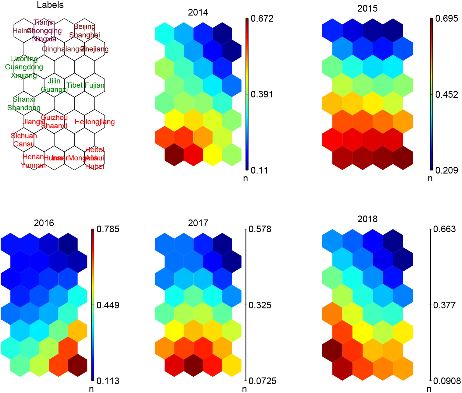
Figure 4.
SOM representation of thirty-one Chinese regions with labels and component planes.
3.2.1Clustering regions w.r.t risk ratings
After risk assessment each region is represented as a risk vector
Figure 4 shows the labels and component planes of map neurons. For easy understanding the regions are marked in different colorings with respect to the cluster information. In specific, the upper neurons belong to Cluster #1 including Beijing, Shanghai, Tianjin, Chongqing, Ningxia, Jiangsu, Hainan, Qinghai, and Zhejiang. The neurons on the bottom correspond to Cluster #3 including Heibe, InnerMongolia, Heilongjiang, Anhui, Jiangxi, Henan, Hubei, Hunan, Sichuan, Guizhou, Yunnan, Shaanxi, Gansu. The other neurons belong to Cluster #2 including Shanxi, Liaoning, Jilin, Fujian, Shandong, Guangdong, Guangxi, Tibet, Xinjiang. Component plane representation visualizes the relative component distribution of the input data for each component (i.e., risk rating of each year in this case study). In this representation, blue values represent relatively small values while red values represent relatively large values. By component planes and corresponding labels along with cluster information we can compare the distribution of risk ratings among clusters. It is observed that the regions in Cluster #1 have relatively low-level risk during five years, those in Cluster #3 have high-level risk and the others have the middle-level risk.
Figure 5.
Clusters of thirty-one Chinese regions using K-means.
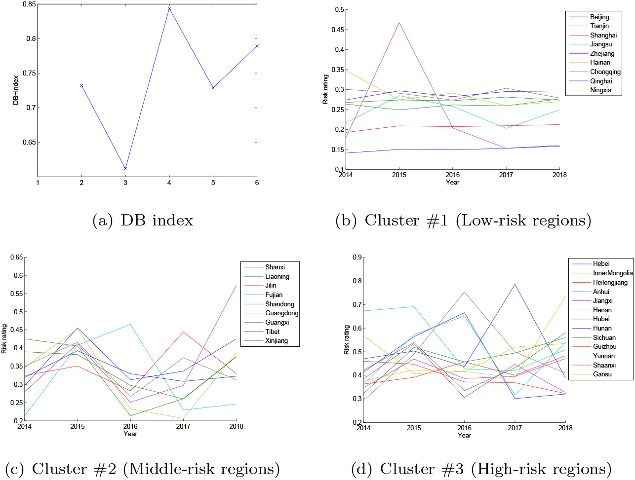
The parallel coordinate of regions is visualized respectively in Fig. 5b–d. The risk rating is mostly between 0.1 and 0.3 for Cluster #1, between 0.2 and 0.45 for Cluster #2, and between 0.3 and 0.8 for Cluster #3. From the vertical (region) view, it is of value to find the main factors on the disparity among regions, for example between Cluster #1 (low-risk regions) and Cluster #3 (high-risk regions) using a quantitative measure.
Given two clusters
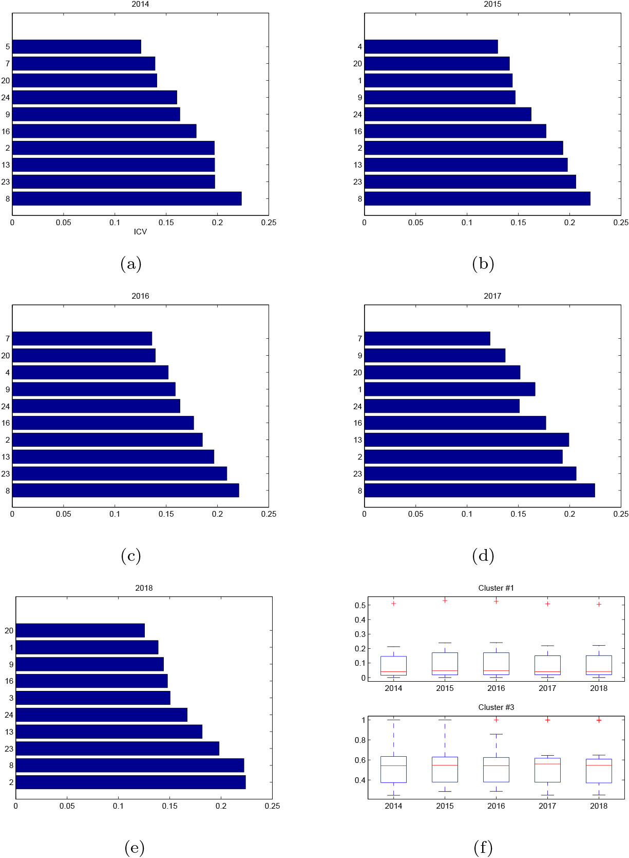
A higher value of ICV indicates a definite contribution on the dissimilarity between two clusters. Figure 6a–e shows the inter-cluster variation (x-axis) of the top 10 contributing factors (y-axis) between Cluster #1 and Cluster #3 from 2014 to 2018. It is observed the yearly risk of regions to natural disasters is impacted by some common factors. In summary, Cultivated land (
Figure 6.
Top 10 contributing indicators in terms of ICV where (a)–(e): Low-risk regions (Cluster #1) vs. High-risk regions (Cluster #3); (f): Box plot of Cultivated land (
3.2.2Clustering regions w.r.t. risk variation
To further explore the similarity of regions with respect to the risk variation, each region is represented as a difference vector
Table 5 shows the clusters of regions with similar risk variation during the five years. The parallel coordinate of regions of five clusters is visualized respectively in Fig. 7. Cluster #1 includes 12 regions, namely Jiangsu, Beijing, Shanghai, Henan, Guizhou, Tianjin, Ningxia, Chongqing, Qinghai, Hainan, Shandong and Tibet. From the parallel coordinate visualization, the risk of these regions are relatively stable despite the minor variation on risk ratings. Cluster #2 includes Shandong and Gansu, characterized by a marked increase in 2018. Cluster #3 comprises 9 regions, namely Shaanxi, InnerMongolia, Liaoning, Zhejiang, Shanxi, Liaoning, Guangdong, Yunan, Sichuan, mostly reaching the highest risk rating in 2015 and lowest rating in 2016. Cluster #4 comprises Hubei, Hebei, Anhui, Fujian, Heilongjiang characterized by a peak in 2016. The other three regions, i.e., Hunan, Jilin, Guanxi, belong to Cluster #5 that keep stable risk during the five years except a distinct peak in the year 2017.
Table 5
Clusters of regional risk variation during five years
| Cluster | Regions | Variation |
|---|---|---|
| #1 | Jiangsu, Beijing, Shanghai, Henan, Guizhou, Tianjin, Ningxia, Chongqing, Qinghai, Hainan, Xinjiang, Tibet |
|
| #2 | Shandong, Gansu |
|
| #3 | Shanxi, InnerMongolia, Liaoning, Zhejiang, Shaanxi, Liaoning, Guangdong, Yunan, Sichuan |
|
| #4 | Hubei, Hebei, Anhui, Fujian, Heilongjiang |
|
| #5 | Hunan, Jilin, Guangxi |
|
Figure 7.
Parallel coordinate visualization of Chinese regions for each cluster.
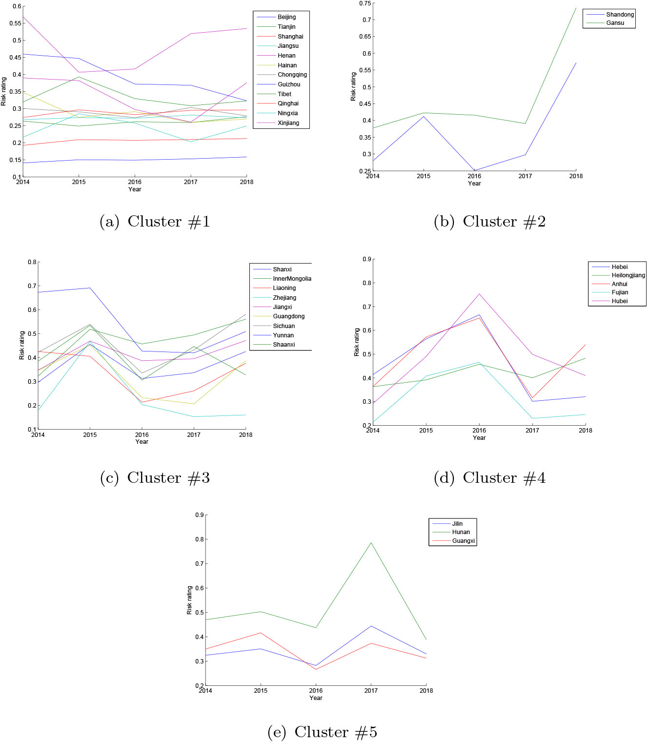
Figure 8.
Top 10 contributing indicators in terms of ICV where (a): High-risk years (2017) vs. Low-risk years (2014–2016, 2018) of Hunan province; (b): High-risk years (2014–2016) vs. Low-risk years (2017–2018) of Hebei province.
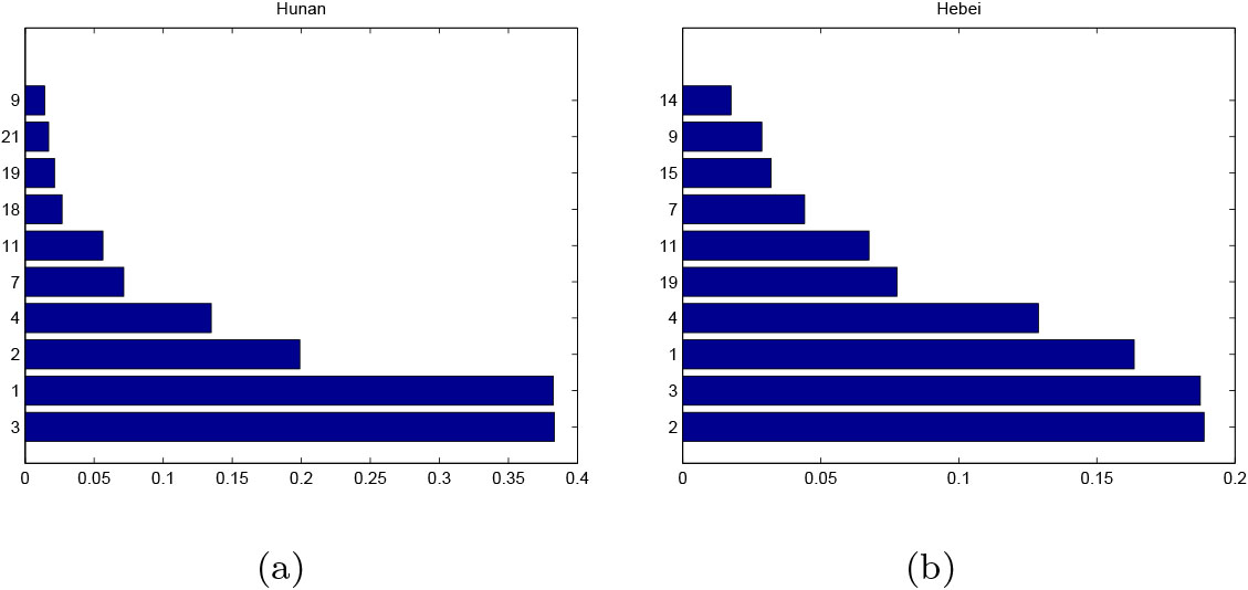
From the horizonal (time) view, it is important to find out the reasons that cause the strong variation on regional risk. Take Hunan and Hebei provinces as example. For the former an abrupt increase of risk is found in the year 2017, and for the latter an abrupt decrease of risk is observed from high-risk years (2014–2016) to low-risk years (2017–2018). This is markedly due to the serve harm of natural disasters represented by Number of people affected by natural disasters (
4.Conclusions and future work
Disasters not only bring threat to people’s safety and property but also cause enormous economical losses and serious influence on social stability. Risk assessment plays an important role in the prediction, warning, and mitigation of disasters. The previous studies of risk assessment are mostly limited in static approaches to risk assessment with inadequate attention on temporal data. As was known temporal data that commonly exists in real world applications is of critical value to analyze the variation of disaster risk. With the increasing interest on the temporal characteristic of data, dynamic risk assessment arises naturally in practice and poses unique challenges for research in analyzing the variation of long-term risk. However there is particularly little related research comparing temporal risk. Given the temporal data related to disaster risk, this paper intents to explore the temporal risk from both horizontal and vertical views, i.e., the temporal variation of risk and the difference of objects.
A two stage risk assessment approach is developed to analyze the variation of risk based on the similarity between risk vectors using a hybrid clustering method integrating SOM with K-means. Firstly the risk of alternatives is measured temporally resulting in a collection of risk vectors. Afterwards based on the similarity measured by a distance metric, SOM groups the alternatives into a number of sets identified by a representative synthetic codebook vector for each group. These groups are further aggregated by K-means to several clusters characterized by risk variation. This approach is applied to two temporal data over several years: infectious diseases (single-objective decision making problem) and regional risk to natural disasters (multi-criteria decision making problem). The clustering of risk vectors implies the similar variation of alternatives and provides insight on understanding the properties of investigated alternatives, for example, the seasonality and co-occurrence of infectious diseases, or the influencing indicators on regional risk to natural disasters. These findings can help decision makers in two folds: (1) to take countermeasures commonly for the group of alternatives within the context of risk reduction and planning; (2) to explore the short-board of alternatives from the set of indicators; (3) to characterize the properties (e.g., periodicity) of variation of disaster risk. In general this study can provide a comprehensive framework for disaster risk analysis, which is helpful for the government and relevant departments to analyze the temporal disaster data, find out the variation characteristics and influencing factors of disaster risk, and therefore formulate disaster prevention and mitigation strategies for disaster prevention and management.
In the future study some research directions will be investigated. Firstly, the variation analysis paradigm can be improved by prediction models for risk prediction and missing value processing with historical data [16, 33] to enhance the capability of emergence management system. Upon the basis of the preliminary findings disclosed in this study, the evolution mechanism behind disaster risk will be further investigated with the aid of domain experts. Secondly, the approach provides a general framework for risk variation analysis. Apart from the methods introduced here, other congener techniques for risk assessment and clustering are easily integrated in the framework. More extensive studies will be performed to ascertain how generalizable and applicable it is to other dynamic risk assessment problems such as COVID-19 pandemic. Nowadays artificial intelligence and machine learning-based models have driven new approaches to drug discovery, vaccine development, and public health awareness [2, 3]. The approach proposed in this paper can be used to mine the relevance between COVID-19 pandemic and existing infectious diseases so as to help discovering new possible treatments and promoting emergency planning.
Acknowledgments
This work was supported by National Office of Philosophy and Social Sciences (19AZD019), National Ethnic Affairs Commission (2020-GMB-015), State Language Commission (E0041918), and Institutes of Science and Development of Chinese Academy of Sciences (Y9X3541H).
References
[1] | Adeloye AJ, Rustum R, Kariyama ID. Kohonen self-organizing map estimator for the reference crop evapotranspiration. Water Resources Research. (2011) ; 47: (8): 192–198. |
[2] | Ahuja AS, Reddy VP, Marques O. Artificial intelligence and COVID-19: A multidisciplinary approach. Elsevier Public Health Emergency Collection. (2020) ; 9: (3). |
[3] | Arshadi AK, Webb J, Salem M, et al. Artificial intelligence for COVID-19 drug discovery and vaccine development. Frontiers in Artificial Intelligence. (2020) ; 3. |
[4] | Aziz N, Sulaiman S, Musirin I, et al. Assessment of evolutionary programming models for single-objective optimization. IEEE 7th International Power Engineering and Optimization Conference (PEOCO). (2013) ; pp. 304–308. |
[5] | Bach DE, Mechler R, Hochrainer S. Dynamic natural disaster risk assessment: A case study for Jamaica. AGU Fall Meeting Abstracts. (2006) . |
[6] | Camacho-Munoz D, Martín J, Santos JL, et al. Occurrence, temporal evolution and risk assessment of pharmaceutically active compounds in Donana Park (Spain). Journal of Hazardous Materials. (2010) ; 183: (1–3): 602–608. |
[7] | Chen L, Huang YC, Bai RZ, Chen A. Regional disaster risk evaluation of China based on the universal risk model. Natural Hazards. (2017) ; 89: (2): 647–660. |
[8] | Chen J, Zhang F, Yang C, et al. Factor and trend analysis of total-loss marine casualty using a fuzzy matter element method. International Journal of Disaster Risk Reduction. (2017) ; 24: : 383–390. |
[9] | Chen N, Chen L, Ma Y, Chen A. Regional disaster risk assessment of China based on self-organizing map: Clustering, visualization and ranking. International Journal of Disaster Risk Reduction. (2018) ; 33: : 196–206. |
[10] | Chen N, Chen L, Tang C, et al. Disaster risk evaluation using factor analysis: A case study of Chinese regions. Natural Hazards. (2019) ; 99: (1): 321–33599. |
[11] | Chen N, Ma Y, Tang C, et al. Risk assessment and comparison of regional natural disasters in China using clustering. Intelligent Decision Technologies. (2020) ; 14: (3): 349–357. |
[12] | Coronese M, Lamperti F, Chiaromonte F, et al. Natural disaster risk and the distributional dynamics of damages. SSRN Electronic Journal. (2018) . |
[13] | Doumpos M, Zopounidis C. Computational intelligence techniques for multicriteria decision aiding: An overview. Multicriteria Decision Aid and Artificial Intelligence, Links, Theory and Applications, Eds., Michael Doumpos and Evangelos Grigoroudis, John Wiley & Sons. (2013) ; 3–24. |
[14] | Ergu D, Kou G, Shi Y, Shi Y. Analytic network process in risk assessment and decision analysis. Computers & Operations Research. (2014) ; 42: : 58–74. |
[15] | Feng C, Li J, Sun W, et al. Impact of ambient fine partic ulate matter (PM2.5) exposure on the risk of influenza-like-illness: A time-series analysis in Beijing, China. Environmental Health. (2016) ; 15: (1): 17. |
[16] | Gourio F. Time-series predictability in the disaster model. Finance Research Letters. (2008) ; 5: (4): 191–203. |
[17] | He H. A simplified approach of drought risk assessment in Poyang Lake basin using real-time precipitation and multi-source remote sensing data. International Symposium on Multispectral Image Processing & Pattern Recognition. International Society for Optics and Photonics. (2015) . |
[18] | Huang DW, Gentili RJ, Katz GE, et al. A limit-cycle self-organizing map architecture for stable arm control. Neural Networks: The Official Journal of the International Neural Network Society. (2016) ; 85: (C): 165–181. |
[19] | Hwang C, Yoon K. Multiple attribute decision making: Methods and applications. New York: Springer-Verlag. (1981) . |
[20] | Kohonen T, Schroeder MR, Huang TS. Self-organizing maps. Springer Berlin Heidelberg, (2001) . |
[21] | Kuo RJ, Ho LM, Hu CM. Integration of self-organizing feature map and k-means algorithm for market segmentation. Computers and Operations Research. (2002) ; 29: (11): 1475–1493. |
[22] | Laerhoven KV. Combining the self-organizing map and k-means clustering for on-line classification of sensor data. Lecture Notes in Computer Science. (2001) ; 2130: : 464–469. |
[23] | Li Z, Fang H, Huang M, et al. Data-driven bearing fault identification using improved hidden Markov model and self-organizing map. Computers & Industrial Engineering. (2018) ; 116: : 37–46. |
[24] | Liu X, Zhang J, Ma D, et al. Dynamic risk assessment of drought disaster for maize based on integrating multi-sources data in the region of the northwest of Liaoning Province, China. Natural Hazards. (2013) ; 65: (3): 1393–1409. |
[25] | Mohammadian M. Artificial intelligence applications for risk analysis, risk prediction and decision making in disaster recovery planning. Artificial Intelligence Applications and Innovations, Springer Berlin Heidelberg. (2012) ; 155–165. |
[26] | Panda M, Jagadev AK. TOPSIS in multi-criteria decision making: A survey. 2nd International Conference on Data Science and Business Analytics (ICDSBA), IEEE Computer Society. (2018) ; pp. 51–54. |
[27] | Peng L, Xia J, Li Z, et al. Spatio-temporal dynamics of water-related disaster risk in the Yangtze River Economic Belt from 2000 to 2015. Resources Conservation and Recycling. (2020) ; 161: : 104851. |
[28] | Roijers DM, Vamplew P, Whiteson S, et al. A survey of multi-objective sequential decision-making. Journal of Artificial Intelligence Research. (2014) ; 48: (1): 67–113. |
[29] | Solidoro C, Bandelj V, Barbieri P, et al. Understanding dynamic of biogeochemical properties in the northern Adriatic Sea by using self-organizing maps and k-means clustering. Journal of Geophysical Research. (2007) ; 112: (C7): C07S90. |
[30] | Vesanto J, Alhoniemi E. Clustering of the self-organizing map. IEEE Transactions on Neural Networks. (2000) ; 11: (3): 586–600. |
[31] | Yu X. Disaster prediction model based on support vector machine for regression and improved differential evolution. Natural Hazards. (2016) ; 85: (2): 1–18. |
[32] | Yano N, Kotani M. Clustering gene expression data using self-organizing maps and k-means clustering. SICE Annual Conference. (2003) ; 3: : 3211–3215. |
[33] | Zhao J, Jin J, Guo Q, et al. Dynamic risk assessment model for flood disaster on a projection pursuit cluster and its application. Stochastic Environmental Research and Risk Assessment. (2014) ; 28: (8): 2175–2183. |
[34] | Zhao J, Jin J, Xu J, et al. Risk assessment of flood disaster and forewarning model at different spatial-temporal scales. Theoretical and Applied Climatology. (2017) ; 132: (2): 791–808. |


