
Ultrasound breast images denoising using generative adversarial networks (GANs)
Abstract
INTRODUCTION:
Ultrasound in conjunction with mammography imaging, plays a vital role in the early detection and diagnosis of breast cancer. However, speckle noise affects medical ultrasound images and degrades visual radiological interpretation. Speckle carries information about the interactions of the ultrasound pulse with the tissue microstructure, which generally causes several difficulties in identifying malignant and benign regions. The application of deep learning in image denoising has gained more attention in recent years.
OBJECTIVES:
The main objective of this work is to reduce speckle noise while preserving features and details in breast ultrasound images using GAN models.
METHODS:
We proposed two GANs models (Conditional GAN and Wasserstein GAN) for speckle-denoising public breast ultrasound databases: BUSI, DATASET A, AND UDIAT (DATASET B). The Conditional GAN model was trained using the Unet architecture, and the WGAN model was trained using the Resnet architecture. The image quality results in both algorithms were measured by Peak Signal to Noise Ratio (PSNR, 35–40 dB) and Structural Similarity Index (SSIM, 0.90–0.95) standard values.
RESULTS:
The experimental analysis clearly shows that the Conditional GAN model achieves better breast ultrasound despeckling performance over the datasets in terms of PSNR
CONCLUSIONS:
The observed performance differences between CGAN and WGAN will help to better implement new tasks in a computer-aided detection/diagnosis (CAD) system. In future work, these data can be used as CAD input training for image classification, reducing overfitting and improving the performance and accuracy of deep convolutional algorithms.
1.Introduction
Medical image analysis plays an important role in breast cancer screening, feature extraction, segmentation, and classification breast lesions locally. There are several breast cancer detection methods, such as Positron Emission Tomography (PET) [1], Computer Tomography (CT) [2] and Magnetic Resonance Imaging (MRI) [3], which are usually used when women are at high risk of breast cancer. Other complementary techniques such as X-ray mammography [4] and ultrasound (US) [5] are more commonly used in screening programs, according to the American Cancer Society.
Among these modalities, US is used as a complementary imaging modality for further evaluation of lesions detected early by mammography due to its non-invasive nature, low cost, safety, portability, and low radiation dose. However, one of its main shortcomings is the poor quality of US image, which is corrupted by random noise added during its acquisition [6, 7], i.e. low contrast and different brightness levels, resulting in increased noise and artifacts that can affect the radiologist’s opinion and diagnosis. US images have a granular appearance called speckle noise, which degrades visual assessment [8], making it difficult for humans to distinguish normal from pathological tissue in diagnostic examinations.
Image denoising techniques, typically low-dose, address this problem [9]. The primary purpose of denoising is to restore the maximum detail of the image by removing excess noise [10], while preserving as much as possible the feature details to benefit the diagnosis and classification of benign, premalignant, and malignant abnormalities (microcalcifications, masses, nodules, tumors, cysts, fibroadenoma, adenosis, and lesions) that may be difficult to identify at first sight or early in the patient.
Thus, denoising medical images is essential before training a classifier based on deep-learning models. Recently, several US denoising techniques based on deep learning have been widely used, such as Convolutional Neural Networks (CNN) [11, 12, 13, 14], Generative Adversarial Networks (GANs) [15, 16, 17], and Autoencoders (AEs) [18, 19], which can recover the original dataset and make it noise-free with better robustness and precision [20]. Deep learning methods have obtained better results in medical imaging in comparison with previous methods such as Wavelet, Wiener, Gaussian [21], Multi-Layer perceptron [22], Dictionary Learning [23], Least Square, Bilateral Filter, Non-Local Mean [24]. Variational approaches [6, 25], because these filters have presented some limitations such as smoothing problems, more computational cost, and inability to preserve information such as edges and textures of images as well as possible [25].
2.Related work
Many traditional denoising filtering techniques have been proposed in the literature to reduce speckle noise [26, 27, 28, 29], which can be categorized into three main types: 1) Spatial domain (Median filter, Mean filter, Adaptive Mean Filter, Frost, Total variation filter, Anisotropic Diffusion, Nonlocal means filter, Linear Minimum Mean Squared Error (LMMSE)). 2) Transform domain (Wiener filter, Low pass filter, Discrete wavelet transform), and 3) Deep learning-based techniques such as Convolutional Neural Networks (CNN), Generative Adversarial Networks (GAN), and Variational Autoencoders (VAEs).
The Spatial and Transform domain methods are computationally simple and fast but sometimes blur the image, and there can be a loss of resolution and low accuracy. Spatial domain filters also have size limitations and window shape problems [28].
However, Deep learning-based models can provide better results compared to these traditional methods, because deep models gives better visual quality by extracting various features of an image as example Li et al. proposed TP-Net [30] as 3D shape classification and segmentation tasks, on a wide range of common datasets, which main contribution is the design of dilated convolution strategy tailored for the irregular and non-uniform structure of 3D mesh data.
Several Generative models (GANs, VAEs) have been successfully used for medical image denoising and data augmentation to improve robustness and prevent overfitting in deep CNN image classification algorithms. Some relevant works are discussed in this section.
Wu et al. [31] implemented a perceptual metrics-guided GAN (PIGGAN) framework to intrinsically optimize generation processing, and experiments show that PIGGAN can produce photo-realistic results and quantitatively outperforms state-of-the-art (SOTA) methods. Pang et al. [32] implemented the TripleGAN model to augment the breast US images. These synthetic images were used to classify breast masses classification using the CNN model, achieving a classification accuracy of 90.41%, sensitivity of 87.94% and specificity of 85.86%. Al-Dhabyani et al. [33] first used breast US data augmentation with GAN and then two deep learning classification approaches: (i) CNN (AlexNet) and (ii) TL (VGG16, ResNet, Inception, and NASNet), achieving in the BUSI dataset an accuracy of 73%, 84%, 82%, 89%, 91% and in Dataset B (UDIAT) an accuracy of 75%, 80%, 77%, 86%, 90% respectively.
Jain et al [34] found that CNN provided comparable and, in some cases, superior performance to Wavelet and Markov Random Field methods. Thus, the Resnet approach proposed by MRDG et al. [11] was used to improve mammography image quality with a peak signal-to-noise ratio (PSNR) of 36.18 and a similar structural index metrix (SSIM) of 0.841. Feng et al [13] implemented a hybrid neural network for US denoising based on the Gaussian noise distribution and VGGNet model to extract the structural boundary information, the results show a (PSNR
Denoising autoencoders based on convolutional layers also perform well for their ability to extract spatial solid correlation [35]. Kaji et al. [9] present an overview describing encoder-decoder networks (pix-2-pix) and cycle GAN as image noise reduction.
Chen et al. [12] proposed the autoencoder and the residual encoder–decoder CNN for low-dose computer tomography (CT) imaging, achieving a good performance index (PSNR of 39.19/SSIM of 0.93 and Root Mean Square Deviation (RMSD) of 0.0097), compared to with other methods in terms of noise suppression, structure preservation, and lesion detection.
However, the use of GANs is considered more stable than autoencoders. GANs are typically used when dealing with images or visual data and work better for signal image processing, such as anomaly detection; on the contrary, VAEs are used for predictive maintenance or security analysis applications [35]. For the previous reason, several GANs have recently been used for data augmentation [36, 37, 38, 39, 40], image super-resolution [21], image translation [9], and noise reduction in the medical field [41, 42].
Zhou et al. [37] proposed a GAN
The most recent deep GAN models used for image denoising are Conditional GAN [43] and Wasserstein GAN [44], which have shown better performance than conventional denoising algorithms [45, 46]. Kim et al. [43] implemented a CGAN network as a medical image denoising algorithm, where the SSIM metric was improved by 1.5 and 2.5 times over conventional methods (Nonlocal Means and Total Variation) respectively, demonstrating a superiority in quantitative evaluation. Vimala et al. [47] proposed an image noise removal in US breast images based on Hybrid Deep Learning Technique, where local speckle noise was destroyed, reaching a signal-to-noise ratios (SNRs) greater than 65 dB, PSNR ratios greater than 70 dB, edge preservation index values more significant than the experimental threshold of 0.48. Zou et al. [37] proposed a network model based on the Wasserstein GAN for image denoising, which improved the noise removal effect.
Based on the previous mentioned our propose integrates concepts from breast cancer research and ultrasound image denoising in a comparative study to evaluate the effect of image pre-processing in improving breast image quality. Improving image quality clarifies patterns, allowing the deep learning model to identify and classify features within the image more accurately. In this study, we explore a novel approach by combining fine-tuning techniques GANs
Denoising of medical images has been used to improve the performance of CNN segmentation and classification algorithms [48, 50]. Ans several CNN methods for general image denoising have been studied ADNet, NERNet, SAnet, CDNet, DRCNN [51], but in this research, as a technical novelty, we combine Conditional GAN
Consenquently, this study aims to: (i) to implement two types of GANs
3.Materials and methods
3.1Databases collection
Three publicly available breast US databases were used in this study: (i) The Breast Ultrasound Images Dataset (BUSI,https://scholar.cu.edu.eg/?q=afahmy/pages/dataset) [52]. This contains data from 600 female patients. The dataset consists of 780 images (133 normal, 437 benign and 210 malignant) with an average image size of 500
A total of 1060 US images were used to train the GAN models; see Table 1.
Table 1
Breast ultrasound public databases
| Dataset | Benign | Malignant | Total |
|---|---|---|---|
| BUSI | 437 | 210 | 647 |
| Dataset A | 100 | 150 | 250 |
| Dataset B | 110 | 53 | 163 |
| Total | 647 | 413 | 1060 |
Figure 1.
Workflow of GANs
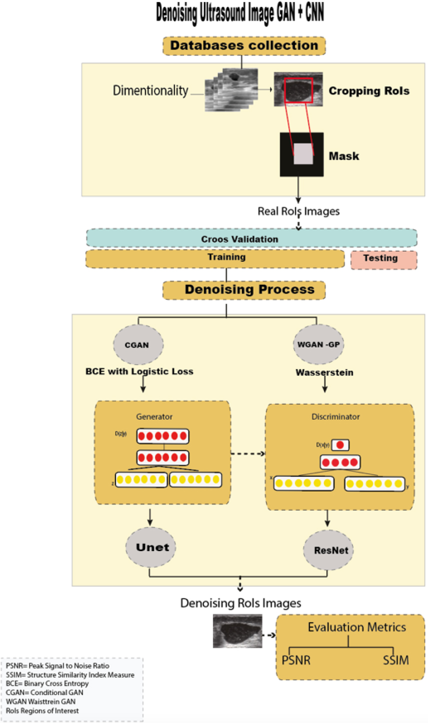
Figure 1 shows the workflow used in denoising breast ultrasound images, which is divided into the following steps: i) Acquisition of public ultrasound databases, ii) Dimensionality and cropping of regions of interest (RoIs), iii) Image denoising using two GANs
3.2Data dimensionality and rois cropping
The torchvision (pytorch) library was used to perform transformations (preserving all features and structure of the images) and to standardize the images to a single dimension (256
According to Wu et al. [36], synthesizing a lesion into RoIs (regions of interest) gives advantages to the generative model, as it generates more realistic lesions, improving subsequent classification performance over traditional augmentation techniques. Thus, automatic RoI extraction was performed on all US images.
Then, using a cross-validation technique, the dataset was randomly divided (with the Sklearn library) into a training set (80%, 851 images) and a testing set (20%, 209 images) for training the GAN models (with the Tensorflow, Keras libraries).
3.3Generative adversarial network
The GAN architecture is represented by a generative (
(1)
Given random noise vector
In this work, we used two ultrasound denoising GANs; (i) conditional GAN and (ii) WGAN, both has been widely used in medical image reconstruction, denoising and data augmentation [56]. Especially CGAN model have been propose as new framework that can largely mitigate the biases and discriminations in machine learning systems while at the same time enhancing the prediction accuracy of these systems [57].
3.3.1Conditional GAN (CGAN)
CGAN was introduced by Douzas et al. [58], as an extension of GAN with conditional information in
(2)
In this work, the generator and discriminator architectures were adapted from [60, 61]. A manual exploration of different configurations in the general hyperparameters was performed to optimize the denoising of breast US images, before selecting and implementing our CGAN model. The selected hyperparameters are: Number of epochs
Figure 2.
CGAN model.
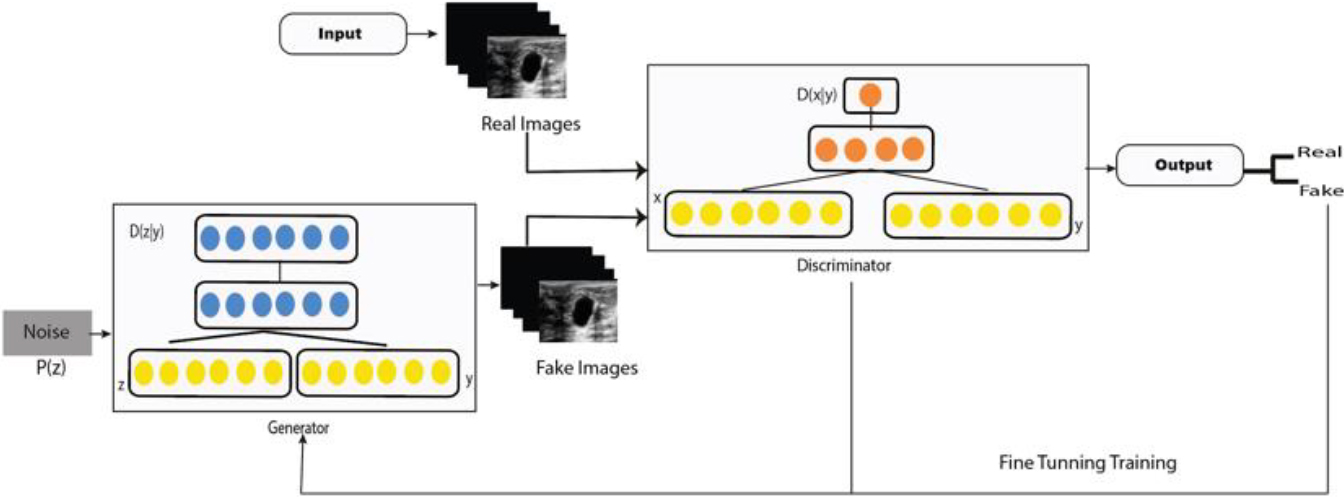
The denoiser discriminator network is based on a Markovian random field (PatchGAN). This consists of an input convolutional layer and 24 convolutional layers followed by batch normalization and a ReLU function (Fig. 2). The output consists of successive convolutional layers 256, 128, 64 and 1. This means that as the input image passes through each of the convolution blocks, the spatial dimension is reduced by a factor of two.
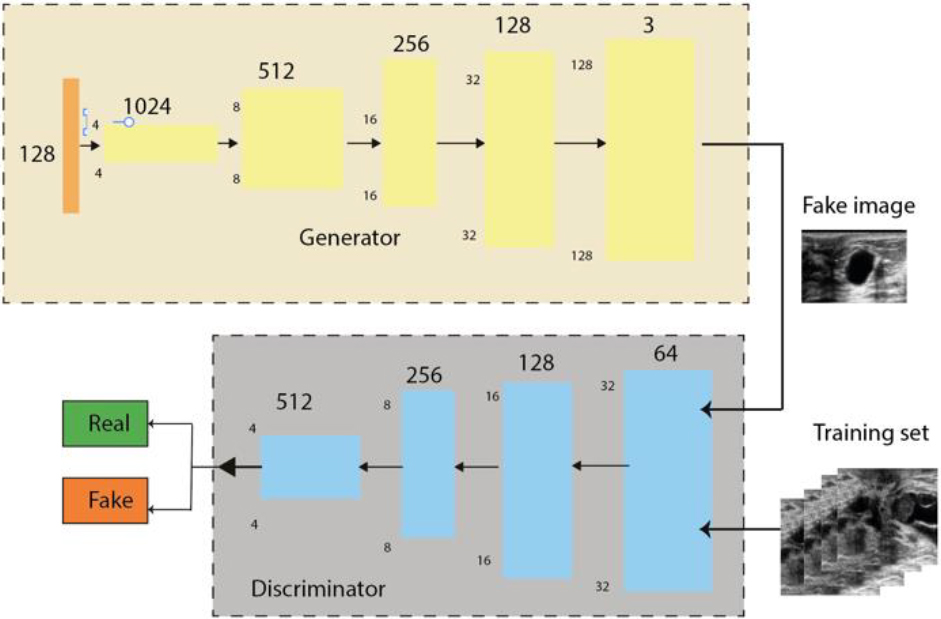
3.3.2Wasserstein GAN (WGAN)
WGAN was introduced by Arjovsky et al. [62], which uses a Wasserstein distance instead of a JS (Jensen-Shanon) or KL (Kullback-Leibler) divergence to evaluate the discrepancy between the distribution distance of noisy and denoised images. It provides a better approximation of the distribution of the observed data in the training data.
The Wassertein (W) model is defined as Eq. (3):
(3)
Where
The denoising generator, was trained by the Resnet model [63]. The generator contains 54 layers, including the input layer, 8 sequential layers of 3 layers each (convolutional layer, normalisation layer and LeakyReLU layer), 7 residual sequences of 4 layers each (transposed convolutional layer, normalisation layer, dropout layer and LeakyReLU layer) and finally a transposed convolutional layer (Fig. 3, Appendix S.3 and S.4).
The denoising discriminator uses the PatchGAN model combined with the Res-Net architecture (convolutional layer, normalization layer and LeakyReLU layer), where the layers were connected directly in a single sequence instead of linking several sequences.
The training phase was carried out with the Google Colab GPU PRO environment, using the Tensorflow and Sklearn libraries for image pre-processing, and PyTorch (CUDA 10.2 graphics cores) to obtain more computational resources and minimise the algorithm execution time. The Tensorflow and Keras libraries were used to train the GAN models.
3.4Evaluation metrics
In addition, most filter techniques use various evaluation metrics such as Mean Square Error (MSE), Root-Mean-Square Error (RMSE), Signal-to-Noise Ratio (SNR), Peak Signal-to-Noise Ratio (PSNR) and Structural Similarity Index (SSIM) to assess image quality.
For quantitative comparison, the PSNR and SSIM [64, 65] were introduced to measure image restoration quality, which is widely used in biomedical applications, especially in mammography and US diagnosis and cancer detection fields.
The PSNR is the metric used to measure the quality of the denoising image when it is corrupted due to noise and blur. A higher value of PSNR indicates a higher quality rate. The standard value of PSNR is 35 to 40 dB (Table 2). The PSNR is calculated by Eq. (4), where is the variance of noise evaluated over the RoI image and is the variance of the filtered image.
(4)
SSIM is a perception-based model that considers the image degradation as perceived change in contrast and structural information. Thus, we can apply this value to assess the quality of any images [66], which lies from 0 to 1 (Table 2).
Table 2
PSNR and SSIM range values
| Quality | PSNR | SSIM |
|---|---|---|
| Low | ||
| Aceptable | 35–40 | 0.90–0.95 |
| High | 40–50 | 0.95–1 |
Figure 3.
WGAN model. Adapted from Hao, Zhuangzhuang et al. (2022).
SSIM index is computed using the correlation coefficient, see Eq. (5).
(5)
Where,
Table 3
Summary of the CGAN and WGAN average comparison results (PSNR and SSIM)
| ID | CGAN | ID | WGAN | ||
|---|---|---|---|---|---|
| PSNR (dB) | SSIM | PSNR (dB) | SSIM | ||
| BUSI | |||||
| img_busi _7 | 39.8433 | 0.974624 | img_busi_7 | 35.0476 | 0.930708 |
| img_busi _56 | 39.8223 | 0.906241 | img_busi_56 | 35.1609 | 0.818753 |
| img_busi _58 | 39.8341 | 0.976325 | img_busi_58 | 35.5627 | 0.952616 |
| img_busi_60 | 40.1839 | 0.978979 | img_busi_60 | 35.2361 | 0.931421 |
| img_busi _70 | 39.7809 | 0.971730 | img_busi_70 | 35.7736 | 0.943916 |
| img_busi _175 | 39.4099 | 0.972768 | img_busi_175 | 35.5431 | 0.942358 |
| img_busi _199 | 39.7116 | 0.929269 | img_busi_199 | 35.3159 | 0.939286 |
| DATASET A | |||||
| img_datasetA_6 | 41.8245 | 0.977663 | img_datasetA_6 | 38.2882 | 0.965505 |
| img_datasetA_11 | 42.1565 | 0.977758 | img_datasetA_11 | 37.7888 | 0.965114 |
| img_datasetA_23 | 41.8171 | 0.978695 | img_datasetA_23 | 38.2925 | 0.967823 |
| img_datasetA_76 | 41.9047 | 0.977636 | img_datasetA_76 | 38.4245 | 0.971207 |
| img_datasetA_188 | 41.9888 | 0.977348 | img_datasetA_188 | 37.2507 | 0.968667 |
| img_datasetA_217 | 41.9424 | 0.978819 | img_datasetA _217 | 37.7399 | 0.971379 |
| img_datasetA_222 | 42.6280 | 0.980217 | img_datasetA_222 | 37.2250 | 0.967832 |
| UDIAT | |||||
| img_udiat_55 | 38.0735 | 0.876853 | img_udiat_55 | 34.1079 | 0.936932 |
| img_udiat_77 | 40.4911 | 0.967255 | img_udiat_77 | 36.4130 | 0.939990 |
| img_udiat_102 | 36.9104 | 0.967851 | img_udiat_102 | 34.5283 | 0.932152 |
| img_udiat_114 | 36.8855 | 0.967821 | img_udiat_114 | 34.1357 | 0.930100 |
| img_udiat_135 | 36.9244 | 0.972911 | img_udiat_135 | 33.3826 | 0.939381 |
| img_udiat_165 | 38.8622 | 0.967638 | img_udiat_165 | 34.3925 | 0.922628 |
| img_udiat_200 | 37.9759 | 0.961544 | img_udiat_200 | 33.7251 | 0.918583 |
| Total average | 38.1873 | 0.961547 | Total average | 33.0068 | 0.919955 |
4.Results
This section presents the most relevant numerical experiments obtained from speckle removal GAN algorithms. First, to improve the algorithm performance, the RoI images were used as GAN training models; in total, we denoising 1060 malignant and benign RoIs. The image quality of the generated data was evaluated with PSNR and SSIM metrics, which are expressed in terms of average value. The most relevant scores are displayed in Table 3; these indicate that the Conditional GAN model showed a significant improvement compared to the other model.
Table 4
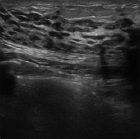
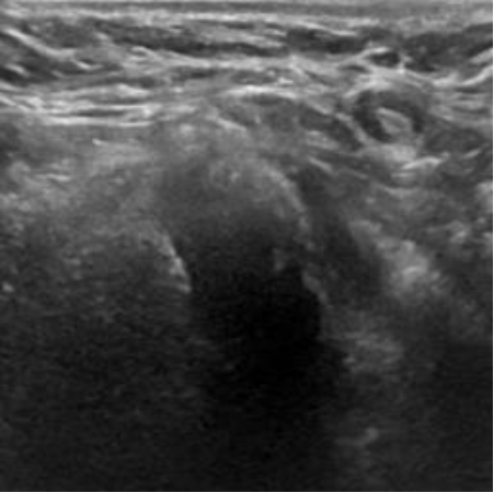
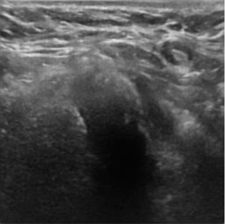
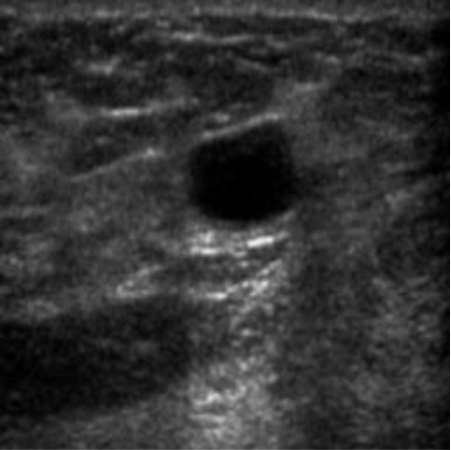
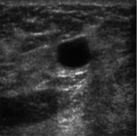
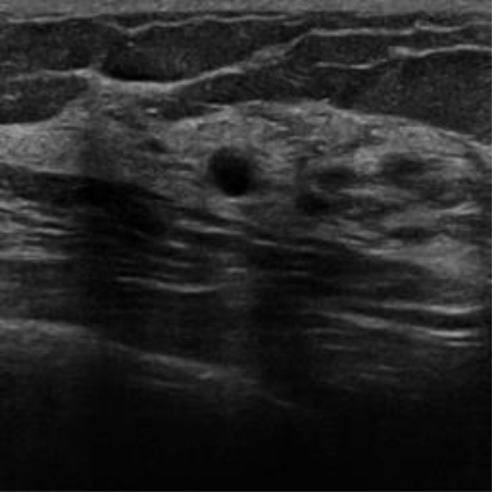
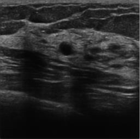
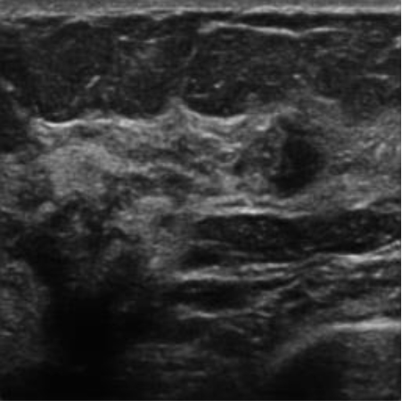
Visual comparison between original ultrasound RoI images and denoising images generated by Conditional GAN and WGAN
| ID | Original | CGAN PSNR/SSIM | WGAN PSNR/SSIM |
|---|---|---|---|
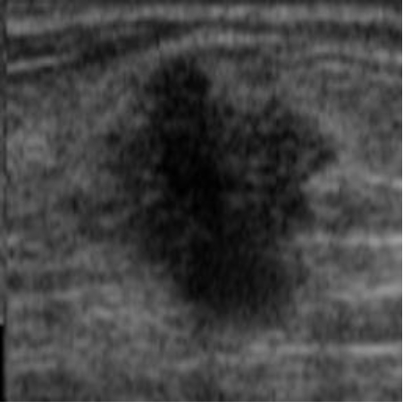
| img_busi_34 |

|  40.18 dB / 0.9789 40.18 dB / 0.9789 |  34.35 dB / 0.9535 34.35 dB / 0.9535 |
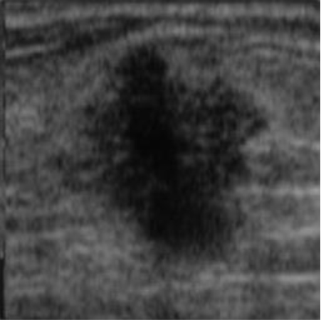
| img_busi _70 |

|  39.78 dB / 0.9717 39.78 dB / 0.9717 |  35.77 dB / 0.9439 35.77 dB / 0.9439 |
| img_busi _175 |
|  39.40 dB / 0.9727 39.40 dB / 0.9727 | 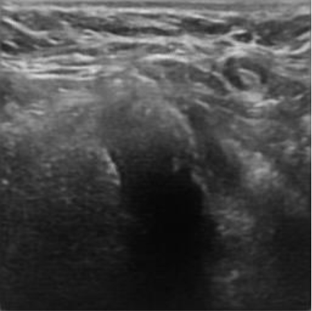 35.54 dB / 0.9423 35.54 dB / 0.9423 |
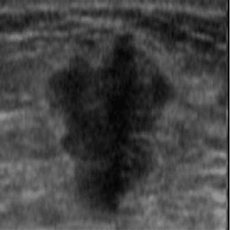
| img_datasetA_6 |
|  41.82 dB / 0.9776 41.82 dB / 0.9776 | 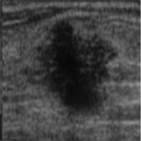 38.28 dB / 0.9655 38.28 dB / 0.9655 |
| img_datasetA_11 |
|  42.15 dB / 0.9777 42.15 dB / 0.9777 |  38.29 dB / 0.9678 38.29 dB / 0.9678 |
|
Table 4, continued | |||
|---|---|---|---|
| ID | Original | CGAN PSNR/SSIM | WGAN PSNR/SSIM |
| img_datasetA_76 |

|  41.90 dB / 0.9776 41.90 dB / 0.9776 | 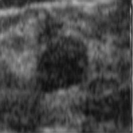 38.42 dB / 0.9712 38.42 dB / 0.9712 |
| img_udiat_77 |
|  38.86 dB / 0.9676 38.86 dB / 0.9676 | 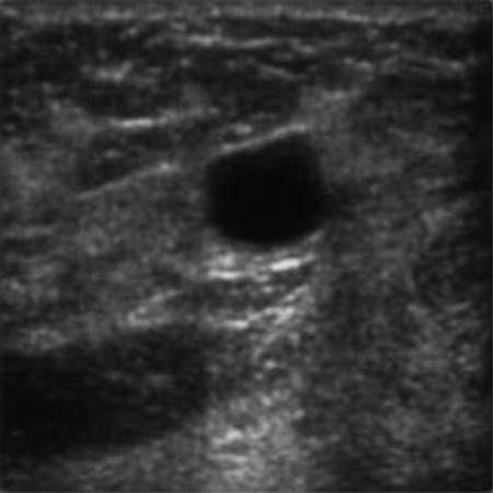 36.41 dB / 0.9399 36.41 dB / 0.9399 |
| img_udiat_165 |
|  40.49 dB / 0.9672 40.49 dB / 0.9672 |  33.38 dB / 0.9393 33.38 dB / 0.9393 |
| img_udiat_200 |

|  37.97 dB / 0.9615 37.97 dB / 0.9615 | 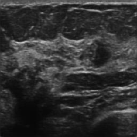 33.72 dB / 0.9185 33.72 dB / 0.9185 |
Although they are visually very similar according to Table 4, the quality values obtained define that the CGAN network achieves a higher mean value in PSNR
To confirm the previous information, the test dataset (239 US images) was used to evaluate the data dispersion of the CGAN and WGAN algorithms using the PSNR and SSIM metrics.
Figure 4.
Dispersion report for PSNR/SSIM metrics. a). CGAN network with PSNR metric. b). CGAN network with SSIM metric. c). WGAN network with PSNR metric. d). WGAN network with SSIM metric.
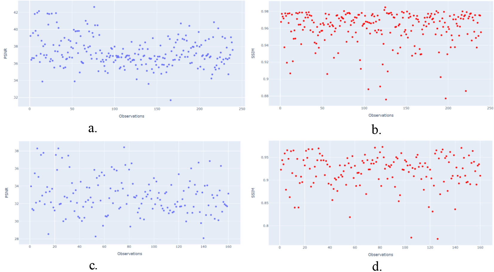
Figure 4a–4d show the statistical results obtained using R software, where a and b show the dispersion data obtained by CGAN. The blue points represent the PSNR metric, which ranges from 30 to 40 dB, and the red points represent the SSIM metric, which ranges from 0 to 1.
Figure 4a and 4b show more signal of better image quality using CGAN network, it means better luminance (PSNR 36–42dB/SSIM 0.85 to 0.98), contrast and structural information in the restructured images by CGAN with respect to WGAN network (PSNR 36–48dB/SSIM 0.85 to 0.95) Fig. 4c and 4d.
5.Discussion
Ultrasound is a complementary technique to mammography and is used for breast cancer detection due to its sensitivity. However, the appearance of speckle noise in US is an interference mode that causes low contrast resolution [33], which makes it difficult to specialize in identifying abnormalities in the breast. In this paper, we trained a pair of GANs combined with CNN architectures as US image denoising, and then evaluated the quality of the denoised images using PSNR and SSIM metrics.
The quality of the denoising image in the Conditional GAN achieved a higher average PSNR (41.03 dB) and SSIM (0.97) in contrast to the average PSNR (35.47 dB) and SSIM (0.93) in the WGAN. Thus, according to the values given in Table 4, the CGAN is consistent with a higher quality image [63] and achieves success in ultrasound denoising images compared to the WGAN. This can be attributed to the fact that CGAN uses the Unet architecture as the generator model and Binary Cross Entropy (BCE) as the loss function (in addition to the L1 loss) [67, 68] to generate real images and provide greater robustness to the model. The Unet has an encoder-decoder network to reconstruct the despeckled image by extracting features from the noisy image to effectively enhance the image features and suppress some speckle noise during the encoding phase [69].
In contrast, WGAN uses Wasserstein distance and Resnet architecture as the generator model with gradient clipping as the loss function to achieve a 1-Lipschitz function. Although this network sometimes avoids the mode collapse problem, resulting in more stable training and less sensitivity to hyperparameter settings (because it is trained based on image distribution loss, rather than image pixel loss) [69], in this work the results generated by WGAN are not statistically significantly better than those generated by CGAN. For the previous reason Gulrajani et al. [70] proposed a WGAN with gradient penalty (GP) to replace the gradient clipping and to enforce Lipschitz continuity, which performs better and more stable training than WGAN with almost no hyperparameter setting
Table 5
Comparison of the accuracy of our denoising method with others GAN and CNN denoising methods
| Author | Method | Main idea | PSNR/SNR (dB) | SSIM | Acc/Sen/Spec (%) |
|---|---|---|---|---|---|
| Eckert et al. [11] | MRDGet | DL method based on CNNs for mammogram denoising to improve the image quality. | 36.18 | 0.841 |
|
| Feng et al. [13] | VGGNet | The network extracts the structure boundaries before and after US image de-speckling | 30.57 | 0.90 |
|
| Pang et al. [32] | TripleGAN | Method to perform data augmentation in breast US images. Then its images are used to classify breast masses using a CNN. |
|
| 90.41/ 87.94/85.86 |
| Al-Dhabyani et al. [33] | AlexNet | US breast masses classification with data augmentation. | 99/-/- | ||
| Vimala et al. [47] | Recurrent Neural Network | Hybrid deep learning technique to remove local speckle noise from breast US images. | 70/65 |
|
|
| Li et al. [72] | CGAN | WGAN loss are combined as the objective loss function to ensure the consistency of denoised image (lung and chest) and real image. | 3326 | 0.92 | |
| Huang, et al. [76] | DUGAN | Deep learning-based model for Low-dose CT denoising | 34.6 | 0.91 |
|
| Elhoseny and Shankar [77] | CNN | Edge preservation and effective noise removal in MRI and CT images. Then, CNN classifier is used to classify the denoised image as normal or abnormal | 47.52 | 0.95 |
|
| Ours | WGAN CGAN | Reduce speckle noise while preserving features and details in breast US images. | 33.00 38.18 | 0.92 0.96 |
These performance differences in performance observed between the CGAN and the WGAN will also help to better implement new tasks in a computer system for detection/diagnosis of benign or malignant breast lesions. The pre-processing steps such as denoising, super resolution, or data augmentation based on deep learning algorithms help to improve the performance and accuracy in terms of clinical relevance in detection, diagnosis, segmentation, or image classification using CNN algorithms.
The main advantage of using GAN algorithms are the quality of the new images produced and the ability to generalize beyond the boundaries of the original dataset to produce new patterns.
Consequently, many researchers have been proposed a deep residual network structure based on GAN networks for image denoising.
Zhang et al. [71] used GANs Unet-based architecture as ultrasound image denoising, with residual dense connectivity and weighted joint loss (GAN-RW) to overcome the limitations of traditional denoising algorithms. The results demonstrated that the noise level (PSNR
The GAN-based combination methods have been applied to different tasks, and have achieved better results. For example [72], proposed a conditional GAN using a WGAN as an objective loss function in medical image denoising, the PSNR/SSIM values (29.4/0.88) demonstrated good results with respect to other state-of-the-art methods, perceiving the structure and details of the images.
Cantero J. [73] investigated two GANs (DCGAN and WGAN-GP) for the generation of synthetic PET (positron emission tomography) breast images. The visual results show that these two architectures can generate sinogram images that confound human evaluators. According to [74] the lower the amount of noise present in the real images the faster the DCGAN network learns to generate high fidelity images, but the results obtained here by WGAN-GP are not significantly better than those produced by DCGAN. In conclusion joint training of denoising and image classification significantly improves the performance of classification. A comparison of the accuracy of our work with more recent methods is shown in Table 5.
Finally, in this study, some limitations were presented, particularly in the availability of private data collection, because only public breast ultrasound databases were used. The implementation of hyperparameters in GAN training is very complex due to the sensitivity of their modification, generating some challenges (collapse mode, convergence, Nash equilibrium, and gradient), which are typical of generative networks. To minimize this problem during the training, it is essential to manually modify some hyperparameters (optimization functions, loss functions, number of epochs, layers, iterations), even to implement new alternatives based on deep convolutional networks to train the generator and the discriminator in a better way.
The research is reproducible, replicable and generalizable, and all code, data and materials have been deposited in the Mendeley repository [75], where the information can be accessed and used by others.
6.Conclusions
In conclusion, in this work CGAN proved to be a useful tool with a better-quality result for denoising breast ultrasound images than the WGAN model. This was obtained by comparing the mean statistical values (PSNR and SSIM) of the GAN models. The higher robustness demonstrated by CGAN is attributed to the fact that the generator uses U-Net encoder-decoder architecture with BCE loss function to remove the speckle noise in a better way than the Resnet architecture used in WGAN. The proposed CGAN technique is particularly useful for small data sets with low variance. These networks are widely used for image generation or data augmentation, but their application in US image denoising is still limited. In future work, other advanced deep learning methods for denoising such as convolutional neural networks and autoencoders will be used, and additional features will be considered in denoising breast images such as PET, thermal, CT, MRI to improve the performance of breast lesion classification algorithms.
Author contributions
Conceptualization Y.J.-G. and V.L.; methodology Y.J.-G.; formal analysis, Y.J.-G., M.J.R.-Á, and V.L.; investigation Y.J.-G and O.V; resources, D.C, Y.S, L.E, A.S, C.S; writing original draft preparation Y.J.-G, O.V; writing manuscript and editing, Y.J.-G., M.J.R.-Á, and V.L.; visualization, Y.J.-G.; supervision, M.J.R.-Á and V.L.; project administration, M.J.R.-Á and V.L.; funding acquisition, M.J. All authors have read and agreed to the published version of the manuscript.
Data availability statement
The data that support the findings of this study are openly available in the Mendeley repository (https:// data.mendeley.com/drafts/g3cmj46xyx) [75].
Abbreviations
| BUSI | Breast Ultrasound Images Dataset |
| BCE | Binary cross entropy |
| CT | Computer Tomography |
| CGAN | Conditional GAN |
| CNN | Convolutional neural network |
| CNR | Contrast to-noise ratio |
| D | Discriminator |
| GAN | Generative adversarial network |
| G | Generator |
| JS | Jensen Shannon |
| KL | Kullback–Leibler |
| KID | Kernel inception distance |
| MRI | Magnetic Resonance Image |
| MSE | Mean Square Error |
| PET | Positron Emission Tomography |
| PSNR | Peak Signal-to-Noise Ratio |
| RMSE | Root-Mean-Square Error |
| SNR | Signal-to-Noise Ratio |
| SSIM | Structural Similarity Index |
| ReLu | Rectified Linear Unit |
| UDIAT | Diagnostic Centre of the Parc Tauli Corporation |
| US | Ultrasound |
| WGAN | Wasserstein GAN |
Supplementary data
The supplementary files are available to download from http://dx.doi.org/10.3233/IDA-230631.
Acknowledgments
This project has been co-financed by the Spanish Government Grant Deepbreast PID2019-107790RB-C22 funded by MCIN/AEI/10.13039/501100011033.
Conflict of interest
The authors declare no conflict of interest.
References
[1] | Y. Satoh et al., Deep learning for image classification in dedicated breast positron emission tomography (dbPET), Ann Nucl Med 36: ((2022) ), 401–410. |
[2] | E.K. Park et al., Machine learning approaches to radiogenomics of breast cancer using low-dose perfusion computed tomography: Predicting prognostic biomarkers and molecular subtypes, Scientific Reports 9: (1) ((2019) ), 17847. |
[3] | Y. Ji et al., Independent validation of machine learning in diagnosing breast Cancer on magnetic resonance imaging within a single institution, Cancer Imaging 19: ((2019) ), 1–11. |
[4] | W.M. Salama and M.H. Aly, Deep learning in mammography images segmentation and classification: Automated CNN approach, Alexandria Engineering Journal 60: (5) ((2021) ), 4701–4709. |
[5] | Y. Xu et al., Medical breast ultrasound image segmentation by machine learning, Ultrasonics 91: ((2019) ), 1–9. |
[6] | T.L. Szabo, Diagnostic ultrasound imaging: inside out, Academic press, (2004) . |
[7] | N.M. Tole, Basic physics of ultrasonographic imaging, World Health Organization, (2005) . |
[8] | S. Wang et al., Speckle noise removal in ultrasound images by first-and second-order total variation, Numerical Algorithms 78: ((2018) ), 513–533. |
[9] | S. Kaji and K. Satoshi, Overview of image-to-image translation by use of deep neural networks: denoising, super-resolution, modality conversion, and reconstruction in medical imaging, Igaku Butsuri: Nihon Igaku Butsuri Gakkai Kikanshi = Japanese Journal of Medical Physics: an Official Journal of Japan Society of Medical Physics 40: (4) ((2020) ), 139–139. |
[10] | I. Njeh et al., Speckle noise reduction in breast ultrasound images: SMU (SRAD median unsharp) approach, Eighth International Multi-Conference on Systems, Signals & Devices. IEEE, (2011) . |
[11] | D. Eckert et al., Deep learning-based denoising of mammographic images using physics-driven data augmentation, Bildverarbeitung für die Medizin 2020: Algorithmen-Systeme-Anwendungen. Proceedings des Workshops vom 15. bis 17. März 2020 in Berlin, Springer Fachmedien Wiesbaden, (2020) . |
[12] | H. Chen et al., Low-dose CT with a residual encoder-decoder convolutional neural network, IEEE Transactions on Medical Imaging 36: (12) ((2017) ), 2524–2535. |
[13] | X. Feng, H. Qinghua and L. Xuelong, Ultrasound image de-speckling by a hybrid deep network with transferred filtering and structural prior, Neurocomputing 414: ((2020) ), 346–355. |
[14] | A.E. Ilesanmi and T.O. Ilesanmi, Methods for image denoising using convolutional neural network: a review, Complex & Intelligent Systems 7: (5) ((2021) ), 2179–2198. |
[15] | E. Kang et al., Cycle-consistent adversarial denoising network for multiphase coronary CT angiography, Medical Physics 46: (2) ((2019) ), 550–562. |
[16] | P. Li et al., Multi-scale residual denoising GAN model for producing super-resolution CTA images, Journal of Ambient Intelligence and Humanized Computing ((2022) ), 1–10. |
[17] | Q. Yang et al., Low-dose CT image denoising using a generative adversarial network with Wasserstein distance and perceptual loss, IEEE transactions on Medical Imaging 37: (6) ((2018) ), 1348–1357. |
[18] | A.S. Ahmed, W.H. El-Behaidy and A.A. Youssif, Medical image denoising system based on stacked convolutional autoencoder for enhancing 2-dimensional gel electrophoresis noise reduction, Biomedical Signal Processing and Control 69: ((2021) ), 102842. |
[19] | M. Daoud et al., Content-based image retrieval for breast ultrasound images using convolutional autoencoders: A feasibility study, 2019 3rd International Conference on Bio-engineering for Smart Technologies (BioSMART), IEEE, (2019) . |
[20] | S.K. Ghosh, B. Biswajit and A. Ghosh, A novel stacked sparse denoising autoencoder for mammography restoration to visual interpretation of breast lesion, Evolutionary Intelligence 14: ((2021) ), 133–149. |
[21] | Y. Jiménez et al., Preprocessing fast filters and mass segmentation for mammography images, Applications of Digital Image Processing XLIV, SPIE, (2021) , pp. 352–362. |
[22] | K.G. Lore, A. Adedotun and S. Soumik, LLNet: A deep autoencoder approach to natural low-light image enhancement, Pattern Recognition 61: ((2017) ), 650–662. |
[23] | X. Chen and S. Qianli, Medical image denoising based on dictionary learning, Biomedical Research (0970-938X) 28: (20) ((2017) ). |
[24] | J. Huang and Y. Xiaoping, Fast reduction of speckle noise in real ultrasound images, Signal Processing 93: (4) ((2013) ), 684–694. |
[25] | M.N. Kohan and B. Hamid, Denoising medical images using calculus of variations, Journal of Medical Signals and Sensors 1: (3) ((2011) ), 184. |
[26] | I. Njeh et al., Speckle noise reduction in breast ultrasound images: SMU (SRAD median unsharp) approach, Eighth International Multi-Conference on Systems, Signals & Devices, IEEE, (2011) , pp. 1–6. |
[27] | R. Dass, Speckle noise reduction of ultrasound images using BFO cascaded with wiener filter and discrete wavelet transform in homomorphic region, Procedia Computer Science 132: ((2018) ), 1543–1551. |
[28] | A.S. Beevi and S. Ratheesha, Speckle Noise Removal Using Spatial and Transform Domain Filters in Ultrasound Images, 2021 7th International Conference on Advanced Computing and Communication Systems (ICACCS), IEEE, (2021) , pp. 291–297. |
[29] | S. Pradeep and P. Nirmaladevi, A review on speckle noise reduction techniques in ultrasound medical images based on spatial domain, transform domain and CNN methods, IOP Conference Series: Materials Science and Engineering, IOP Publishing, (2021) , pp. 012116. |
[30] | P. Li et al., TPNet: A Novel Mesh Analysis Method via Topology Preservation and Perception Enhancement, Computer Aided Geometric Design ((2023) ), 102219. |
[31] | H. Wu et al., Perceptual metric-guided human image generation, Integrated Computer-Aided Engineering 29: (2) ((2022) ), 141–151. |
[32] | T. Pang et al., Semi-supervised GAN-based radiomics model for data augmentation in breast ultrasound mass classification, Computer Methods and Programs in Biomedicine 203: ((2021) ), 106018. |
[33] | W. Al-Dhabyani et al., Deep learning approaches for data augmentation and classification of breast masses using ultrasound images, Int. J. Adv. Comput. Sci. Appl 10: (5) ((2019) ), 1–11. |
[34] | V. Jain and S. Seung, Natural image denoising with convolutional networks, Advances in Neural Information Processing Ssystems 21: ((2008) ). |
[35] | S.D. Wickramaratne and M.S. Mahmud, Conditional-GAN based data augmentation for deep learning task classifier improvement using fNIRS data, Frontiers in Big Data 4: ((2021) ), 659146. |
[36] | E. Wu et al., Conditional infilling GANs for data augmentation in mammogram classification, Image Analysis for Moving Organ, Breast, and Thoracic Images: Third International Workshop, RAMBO 2018, Fourth International Workshop, BIA 2018, and First International Workshop, TIA 2018, Held in Conjunction with MICCAI 2018, Granada, Spain, September 16 and 20, 2018, Proceedings 3, Springer International Publishing, (2018) , pp. 98–106. |
[37] | Z. Zhou et al., Image quality improvement of hand-held ultrasound devices with a two-stage generative adversarial network, IEEE Transactions on Biomedical Engineering 67: (1) ((2019) ), 298–311. |
[38] | L. Bargsten and A. Schlaefer, SpeckleGAN: a generative adversarial network with an adaptive speckle layer to augment limited training data for ultrasound image processing, International Journal of Computer Assisted Radiology and Surgery 15: ((2020) ), 1427–1436. |
[39] | H.G. Khor et al., Ultrasound speckle reduction using wavelet-based generative adversarial network, IEEE Journal of Biomedical and Health Informatics 26: (7: ) ((2022) ), 3080–3091. |
[40] | D. Mishra et al., Ultrasound image enhancement using structure oriented adversarial network, IEEE Signal Processing Letters 25: (9) ((2018) ), 1349–1353. |
[41] | F. Carrara et al., Combining gans and autoencoders for efficient anomaly detection, 2020 25th International Conference on Pattern Recognition (ICPR). IEEE, (2021) , pp. 3939–3946. |
[42] | Y. Yao et al., Conditional Variational Autoencoder with Balanced Pre-training for Generative Adversarial Networks, 2022 IEEE 9th International Conference on Data Science and Advanced Analytics (DSAA), IEEE, (2022) , pp. 1–10. |
[43] | H.J. Kim and D. Lee, Image denoising with conditional generative adversarial networks (CGAN) in low dose chest images, Nuclear Instruments and Methods in Physics Research Section A: Accelerators, Spectrometers, Detectors and Associated Equipment 954: ((2020) ), 161914. |
[44] | X. Zou et al., WGAN-Based Image Denoising Algorithm, Journal of Global Information Management (JGIM) 30: (9) ((2022) ), 1–20. |
[45] | V.K. Singh et al., Conditional generative adversarial and convolutional networks for X-ray breast mass segmentation and shape classification, Medical Image Computing and Computer Assisted Intervention – MICCAI 2018: 21st International Conference, Granada, Spain, September 16–20, 2018, Proceedings, Part II 11. Springer International Publishing, (2018) , pp. 833–840. |
[46] | Y. Zhang, C. Hu and K. Wenchi, Medical image denoising, Biomedical Image Synthesis and Simulation, Academic Press, (2022) , 255–278. |
[47] | B.B Vimala et al., Image Noise Removal in Ultrasound Breast Images Based on Hybrid Deep Learning Technique, Sensors 23: (3) ((2023) ), 1167. |
[48] | D. Khaledyan, et al., Enhancing breast ultrasound segmentation through fine-tuning and optimization techniques: Sharp attention UNet, Plos One 18: (12) ((2023) ), e0289195. |
[49] | S. Zama et al., Clinical Utility of Breast Ultrasound Images Synthesized by a Generative Adversarial Network, Medicina 60: (1) ((2023) ), 14. |
[50] | M. Li et al., Medical image analysis using deep learning algorithms, Frontiers in Public Health 11: ((2023) ), 1273253. |
[51] | A.E. Ilesanmi and T.O. Ilesanmi, Methods for image denoising using convolutional neural network: a review, Complex & Intelligent Systems 7: (5) ((2021) ), 2179–2198. |
[52] | W. Al-Dhabyani et al., Dataset of breast ultrasound images, Data in Brief 28: ((2020) ), 104863. |
[53] | P.S. Rodrigues, Breast ultrasound image, Mendeley Data 110.17632. ((2017) ). |
[54] | M.H. Yap et al., Automated breast ultrasound lesions detection using convolutional neural networks, IEEE Journal of Biomedical and Health Informatics 22: (4) ((2017) ), 1218–1226. |
[55] | I. Goodfellow et al., Generative adversarial networks, Communications of the ACM 63: (11) ((2020) ), 139–144. |
[56] | M. Gong et al., Generative adversarial networks in medical image processing, Current Pharmaceutical Design 27: (15) ((2021) ), 1856–1868. |
[57] | A. Abusitta, E. Aïmeur and O.A. Wahab, Generative adversarial networks for mitigating biases in machine learning systems, arXiv preprint arXiv:190509972. ((2019) ). |
[58] | G. Douzas and F. Bacao, Effective data generation for imbalanced learning using conditional generative adversarial networks, Expert Systems with Applications 91: ((2018) ), 464–471. |
[59] | Y. Yu et al., Unsupervised representation learning with deep convolutional neural network for remote sensing images, Image and Graphics: 9th International Conference, ICIG 2017, Shanghai, China, September 13–15, 2017, Revised Selected Papers, Part II 9. Springer International Publishing, (2017) , pp. 97–108. |
[60] | P. Isola et al., Image-to-image translation with conditional adversarial networks, Proceedings of the IEEE conference on computer vision and pattern recognition, (2017) , pp. 1125–1134. |
[61] | O. Ronneberger, P. Fischer and T. Brox, U-net: Convolutional networks for biomedical image segmentation, Medical Image Computing and Computer-Assisted Intervention–MICCAI 2015: 18th International Conference, Munich, Germany, October 5-9, 2015, Proceedings, Part III 18, Springer International Publishing, (2015) , pp. 234–241. |
[62] | M. Arjovsky, S. Chintala and L. Bottou, Wasserstein generative adversarial networks, International conference on machine learning, PMLR, (2017) , pp. 214–223. |
[63] | K. He et al., Deep residual learning for image recognition, Proceedings of the IEEE conference on computer vision and pattern recognition, (2016) , pp. 770–778.. |
[64] | A. Obukhov and M. Krasnyanskiy, Quality assessment method for GAN based on modified metrics inception score and Fréchet inception distance, Software Engineering Perspectives in Intelligent Systems: Proceedings of 4th Computational Methods in Systems and Software 2020, Vol. 14, Springer International Publishing, (2020) , pp. 102–114. |
[65] | S. Rajkumar and G. Malathi, A comparative analysis on image quality assessment for real time satellite images, Indian J. Sci. Technol 9: (34) ((2016) ), 1–11. |
[66] | S. Rajkumar and G. Malathi, A comparative analysis on image quality assessment for real time satellite images, Indian J. Sci. Technol 9: (34) ((2016) ), 1–11. |
[67] | M.T. Martinez and O.N. Heiner, Conditional generative adversarial networks for solving heat transfer problems, No. SAND-2020-10569, Sandia National Lab, (SNL-NM), Albuquerque, NM (United States), (2020) . |
[68] | N. Mohammadi, M.M. Doyley and M. Cetin, Regularization by adversarial learning for ultrasound elasticity imaging, 2021 29th European Signal Processing Conference (EUSIPCO), IEEE, (2021) , pp. 611–615. |
[69] | Y. Lan and X. Zhang, Real-time ultrasound image despeckling using mixed-attention mechanism based residual UNet, IEEE Access 8: ((2020) ), 195327–195340. |
[70] | I. Gulrajani et al., Improved training of wasserstein gans, Advances in Neural Information Processing Systems 30: ((2017) ). |
[71] | L. Zhang and J. Zhang, Ultrasound image denoising using generative adversarial networks with residual dense connectivity and weighted joint loss, PeerJ Computer Science 8: ((2022) ), e873. |
[72] | Y. Li et al., A novel medical image denoising method based on conditional generative adversarial network, Computational and Mathematical Methods in Medicine 2021: ((2021) ), 1–11. |
[73] | L. Cantero, A GAN approach to synthetic PET imaging generation for breast cancer diagnosis, Master’s thesis, Universitat Oberta de Catalunya, (2021) . |
[74] | Y. Lei, J. Zhang and H. Shan, Strided self-supervised low-dose CT denoising for lung nodule classification, Phenomics 1: ((2021) ), 257–268. |
[75] | Y. Jimenez et al., Ultrasound Breast images denoising using Generative Adversarial Networks (GANs), Mendeley Data V1: , ((2023) ). |
[76] | Z. Huang et al., DU-GAN: Generative adversarial networks with dual-domain U-Net-based discriminators for low-dose CT denoising, IEEE Transactions on Instrumentation and Measurement 71: ((2021) ), 1–12. |
[77] | M. Elhoseny and K. Shankar, Optimal bilateral filter and convolutional neural network based denoising method of medical image measurements, Measurement 143: ((2019) ), 125–135. |


