
Content-aware data distribution over cluster nodes
Abstract
Proper data items distribution may seriously improve the performance of data processing in distributed environment. However, typical datastorage systems as well as distributed computational frameworks do not pay special attention to that aspect. In this paper author introduces two custom data items addressing methods for distributed datastorage on the example of Scalable Distributed Two-Layer Datastore. The basic idea of those methods is to preserve that data items stored on the same cluster node are similar to each other following concepts of data clustering. Still, most of the data clustering mechanisms have serious problem with data scalability which is a severe limitation in Big Data applications. The proposed methods allow to efficiently distribute data set over a set of buckets. As it was shown by the experimental results, all proposed methods generate good results efficiently in comparison to traditional clustering techniques like k-means, agglomerative and birch clustering. Distributed environment experiments shown that proper data distribution can seriously improve the effectiveness of Big Data processing.
1.Introduction
Key-based data distribution is today a standard of data distribution in Big Data systems. It provides the uniform data distribution over a set of cluster nodes. However, this approach does not particularly take into consideration the actual content of the data. Consequently, similar data items may be randomly distributed. On the other hand, content aware data distribution can be used to improve the effectiveness of distributed processing.
Organizing data items based on their similarity is a well known classification problem typically solved using data clustering. Despite the years of research in the area of data clustering, it is still a popular and non-trivial problem especially for contemporary enormous data sets. Nowadays, many Big Data processing techniques can not be efficiently performed without using the parallel and distributed systems. However, most of the traditional algorithms require availability of the whole data set in a centralized unit which seriously complicates the matter [3]. High volume of data, data variety, different data structure or high-dimensional data contribute to the high complexity of the problem. It was already proved that there is no best clustering method [21].
Scalable Distributed 2-Layer Datastore (SD2DS) is a fully scalable system for storing and processing Big Data. The aim of this work is to develop a new addressing method for SD2DS that will automatically perform basic data clustering without the loss of performance and scalability. Previously used addressing methods focused on proper data distribution without paying particular attention to clustering, thereby omitting data items similarity or their meaning in general. The proposed addressing methods that group similar data items on the same distributed system node are defined as static data clustering. The term static in this context means that the method is performed during the process of inserting a data item into the datastore and never changes. It seems to be a serious limitation because the clustering method is strictly defined and it can not be changed during the use of datastore. Moreover, the data can not be treated in any other way. On the other hand, it can be considered as an entry point for other data exploration techniques, what is a valuable advantage.
This paper is organized as follows. Section 2 describes related works. In Section 3 author briefly introduces SD2DS and its data processing model. Section 4 presents the new approaches to distributing data items in Big Data environments based on SD2DS. Experimental evaluation of the proposed approaches is presented in Section 5. The paper ends with conclusions.
2.Related works
Data clustering is a powerful tool commonly used in many expert systems. Not only the basic clustering methods [18] but also the complicated ones [47, 14] have been well known for many years. Most of them were developed for relatively small representative data sets and do not scale well or even are inefficient with Big Data sets [18]. There are many works on both developing new methods and adapting the existing ones for parallel and distributed environments. Most of the traditional clustering methods (like K-means) present a great challenge while using them in distributed environment. Mostly they require access to the whole data set to perform their tasks. A very interesting idea to perform clustering for Big Data is to use some variation of space partition clustering [5]. In that case each data node may be responsible for managing a set of data items that occupies a specific area of the whole space. Additionally, merging data items from a group of nodes (or dividing data items into some nodes) allows to aggregate the data items similarly as using hierarchical clustering [6]. Newly created algorithms often utilize the deep learning approach to data clustering. The most well known examples are based on Self Organizing Maps [42] or Expectation-Maximization [17].
The increasing growth of gathered data sets forces development of novel techniques of data mining. A lot of them was utilized to deal with data sets that are beyond the possibilities of a single machine. Data streaming and parallelization are two the most popular approaches of dealing with really huge data sets.
Apart from great advantages, like reducing memory consumption and ease of development, clustering using streaming frameworks has also serious drawbacks: often allows to process each data item only once (one-pass approach) and can be sensitive to the order of the data items. To overcome this problem an evolving approach is often utilized which provides the concept of time windows allowing to create a micro-clusters from a continuous set of data items. Sliding window is the most common approach of utilizing those time windows [7, 49]. It can be suitable for time evolving data [34] as it can properly handle the drifting problem [9]. CluStream [1] is one of the well known stream based clustering method. It divides the clustering process into two phases: online process, for statistical summary of the portion of the data, and offline process, for final clustering with user defined time period. DenStream presents a serious improvement in terms of detection of arbitrary shape clusters, detection of the number of clusters and noise insensitivity by detecting the density of the clusters [7]. HPStream allows to build proper cluster thanks to taking into consideration most recent data items and eliminating outdated ones [49]. This approach can not only improve the quality of the cluster but also allows to formulate the queries considering specified time periods [49].
There are many parallel clustering algorithms both versions of original algorithms and algorithms built from scratch [39]. Popular techniques, known from traditional clustering algorithms, like sample clustering, dimension reduction [11] or hierarchical approach, which allow to divide and/or merge data subsets, present the natural way to perform parallel computation. The parallelization of the most recognizable K-means method was widely discussed (e.g. [48]). Additionally, parallel version of DBSCAN can be found in [44], while parallel version of BIRCH was proposed in [12]. There are also many methods specially developed for custom needs in the areas like bio-informatics [30] or for cosmological data [2]. Many of them were created based on distributed PCA method [26] or by merging the intermediate outcomes [28]. A good overview of parallel clustering methods can be found in [20].
While the data distribution becomes the most popular today for dealing with high volume of data, it still has a lot of disadvantages. Most of the approaches on clustering Big Data today is usually built on top of the MapReduce framework [10] or similar systems like Apache Spark [16]. While MapReduce has some serious limitations itself [19], it also often requires to discard the referenced well known algorithms in favour of introducing specific ones. This might be the serious issue for many applications which require proven and well described algorithms. Additionally, methods based on MapReduce [10] suffer from large network transfer [45]. Moreover, data distribution may also cause the problem of local optimum convergence [35]. Additionally, most of the distributed systems need some form of central node, which may become bottle-neck or even a single point of failure. Alternatively, they will need a very complex distributed consensus algorithm [3].
The typical approach to distribute data items over a set of distributed system nodes uses one of the following strategies:
• Key or keys based – each data item is identified by a unique key (systems such as: Dynamo [37] or Hazelcast),
• name based – typically used by distributed files systems (like in Google File System [13], Hadoop File System [36] or internal storage of Apache Spark [46]),
• topic based – identified by a name of the topic which data was published to (like in Apache Kafka [40]).
Well known classification of NoSQL datastorages divides those systems into four categories: key-value [38], column-based [8], graph-based [4] and document-based [33]. Despite the differences in internal data structure, data items are still most commonly identified by a unique key. For example MongoDB usually identifies documents by keys [32], Neo4J typically identifies the nodes by ids [29], similarly HBase assigns rowids to the rows stored in tables [43].
All in all, most of those solutions do not even consider the content of the data during data distribution process. However, distributing data items based on their content can seriously improve processing methods. For example, processing tasks may be specially prepared for each data partition and do not need to assume that data items are mixed. As a striking example, data partition can be treated as noise and omitted during processing when the number of data items is less than some predefined value. This approach is expected to significantly improve distributed calculations in comparison to the typical approaches known from MapReduce, Apache Spark or Apache Kafka.
3.Scalable Distributed Two Layer Datastore
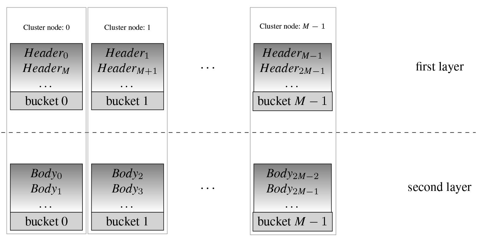
Scalable Distributed Two Layer Datastore (SD2DS) [22] proved to be a very efficient solution for storing massive data sets. The basic idea of the SD2DS is the division of the data item (called component) into two separate parts: the component header (identified by a unique key
Figure 1.
The architecture of SD2DS consisting of
3.1Distributed Linear Hashing
The distributed addressing for an appropriate header is performed by Distributed Linear Hashing (
(1)
and
(2)
where:
•
•
•
This approach can alternatively be presented as determining the data item address based on the least significant bits of its key.
An additional parameter (
(3)
Even when the values of the state (
[h] The addressing function for
3.2SD2SD processing model
The processing model for SD2DS [23] was developed for high dimensional Big Data sets. Such a form of data items is still a big challenge in many data exploration techniques [15]. Each data item, that is stored in the second layer of SD2DS, is represented as a feature vector:
(4)
where:
•
•
•
This simple data representation is suitable for most of the data exploration needs. However, addressing those data items may be really challenging. As stated above,
SD2DS allows executing distributed processing jobs using mechanism similar to MapReduce paradigm [23]. It divides the jobs into block function, which is executed on each data items partition and aggregate function which gathers the intermediate and final results. Those tasks are considered as equivalents to map and reduce functions respectively.
3.3Simple static clustering in SD2DS (SD2DS_S)
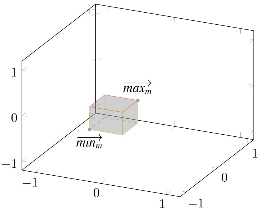
The paper [24] firstly stated the above mentioned problem and introduced a basic solution for it which is now described as simple static clustering (SD2DS_S). The basic idea in the proposed approach is to treat each bucket as a part of the multi–dimensional space:
(5)
where
(6)
(7)
Each data item is managed by the bucket that is responsible for a disjoint part of the space which creates a partitional, hard clustering solution. The similarity of the data items is measured by the simple euclidean distance. However, picking an appropriate distance measure can seriously improve the clustering result, the euclidean distance is chosen as the most typically used. This measure is used in all the proposed methods in the paper. Additionally, by utilizing different
Figure 2.
The graphical representation of a bucket (
Although the simple static clustering proved to be an efficient and effective method it still has problems with arbitrary shape clusters. This paper is focused on developing a solution that can overcome this limitation preserving both effectiveness and scalability.
4.Data distribution in SD2DS
4.1Advanced static clustering (SD2DS_A)
SD2DS_S method presented in the previous section can only introduce clusters of rectangular shapes (or hyper-rectangular shapes in general) which is a very serious restriction. To overcome this issue other approaches should be investigated.
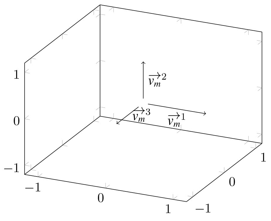
The proposed solution of this problem is to treat each first layer bucket description as a sequence of vectors:
(8)
In such a way all points that lie in the area designated by this sequence of vectors (
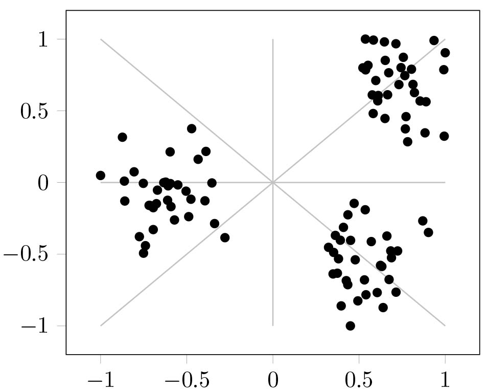
Figure 3.
The graphical representation of a bucket (
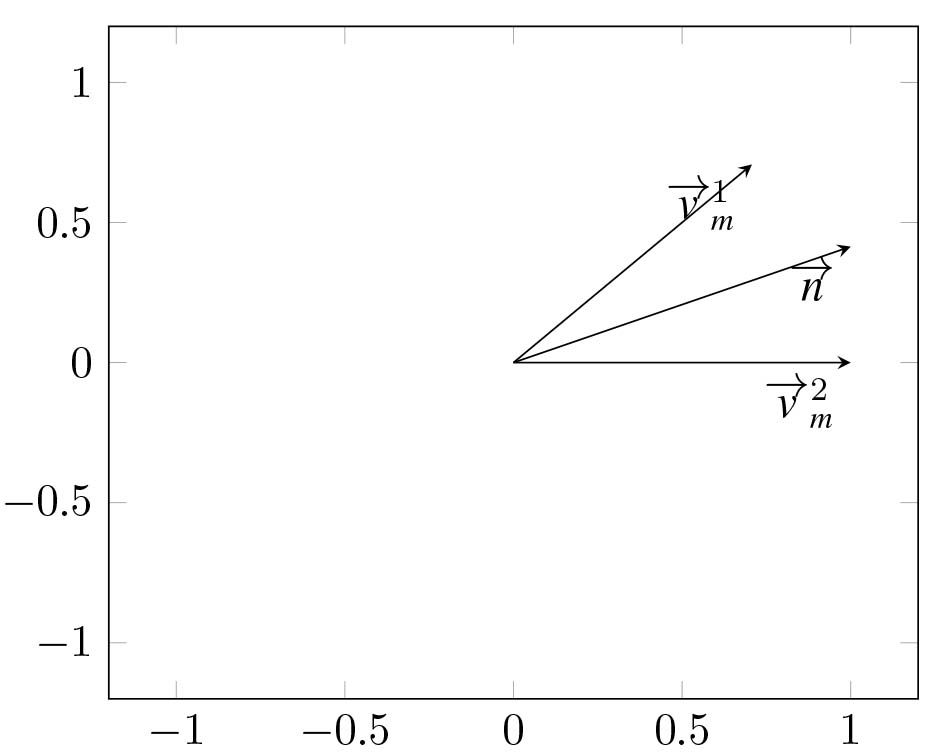
4.1.1Component addressing
In order to perform the component addressing it is needed to determine if an examined data item lies between two vectors:
(9)
where
•
•
The above equation can be resolved as:
The whole process of determining the data item membership to the designated bucket can be described as:
(10)
This approach can be also defined as operations in the polar coordinate system. In that case a bucket is represented as a radius and an appropriate angle which cover part of the whole space. In order to stay consistent with other proposed methods and to avoid conversion between coordinate systems the Cartesian interpretation is preferable.
The data item addressing process is conducted hierarchically, similarly as in the SD2DS_S described in the previous section. The SD2DS_A method is suitable for the cases where
KwDowntodownto
The overall procedure of addressing data item in SD2DS_A is presented in Algorithm 4.1.1.
4.1.2Bucket split
Similarly, as in the SD2DS_S the split of a bucket may be considered as a division of space that is managed by the bucket. The graphical representation of a bucket split in two–dimensional space is presented in Fig. 4.
Figure 4.
Graphical representation of a split of a bucket for advanced static clustering.
The creation of a new vector that represents the border between the old and newly created bucket is simply a normalized vector obtained by adding two vectors:
(11)
In two-dimensional space the original bucket is described as:
(12)
while the newly created bucket is described as:
(13)
The overall procedure of splitting bucket in d-dimensional space is presented in Algorithm 4.
Figure 5.
An example of SD2DS_A clustering structure (
4.2Combined static clustering (SD2DS_C)
More complicated shapes of cluster can still pose a challenge to both SD2DS_S and SD2DS_A methods. The SD2DS_A method will still generate not accurate results when the cluster will occupy the centre of the coordinate system. This problem may be resolved by combining those two techniques in such a way that the SD2DS_S is used to translate the local coordinate system to properly handle that situation. In order to achieve that, a threshold (
•
•
The threshold value needs to fulfil the requirement:
(14)
where:
•
The graphical representation of a SD2DS_C is presented in Fig. 6. As it can be seen, the SD2DS_C introduces a centre of a local coordinate system for each bucket similarly as in SD2DS_S. The centre of a local coordinate system is defined by bucket on the level
Figure 6.
SD2DS_C clusters structure (
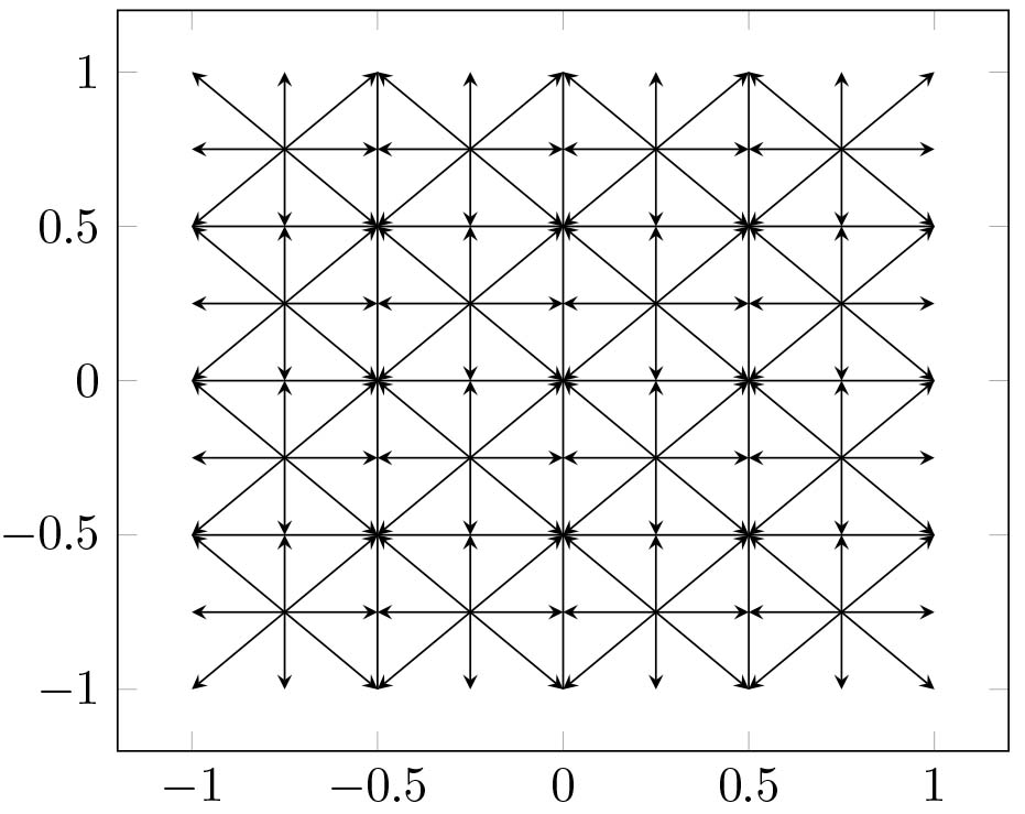
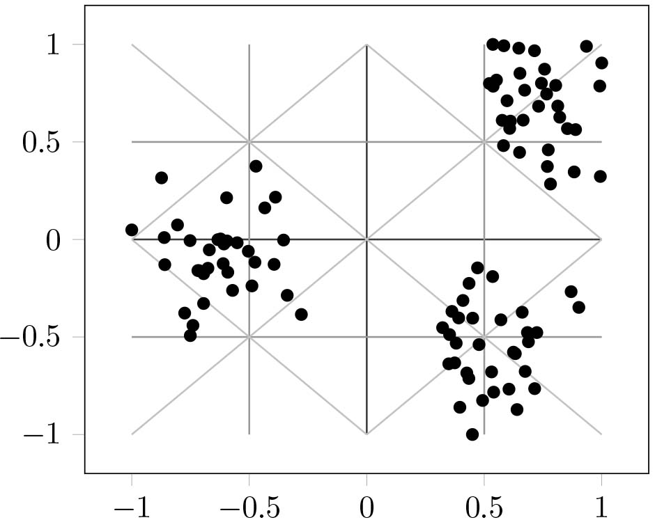
Figure 7.
An example of SD2DS_C structure (
5.Experimental results
The evaluation was conducted both using simulations and Big Data distributed environment. By using simulations it was possible to evaluate the data distribution, quality of distribution and efficiency in comparison with the traditional clustering methods that are not suitable for distributed environments. On the other hand, utilizing distributed implementation allows to evaluate methods on a Big Data set in environment with many clients running simultaneously on SD2DS.
The proposed advanced (SD2DS_A) and combined static clustering (SD2DS_C) were evaluated by comparing them with simple static clustering (SD2DS_S) as well as with traditional clustering techniques like k-means (depicted as Kmeans in figures), agglomerative hierarchical clustering (Agglomerative in figures) and birch clustering (Birch in figures). The implementation from a scikit-learn package [31] was used for all the traditional methods. In the next sub-sections of this paper the quality evaluation was presented. Moreover, the speed and scalability evaluation were shown. To perform evaluation different data sets were randomly generated with a variety of noise ratios, different data-dimensionality and different sizes. The parameters of random datasets are presented in Table 1. Those synthetic data sets allow to deeply analyse both the performance and quality of the proposed solutions.
Table 1
Parameters of synthecic datasets
| Shape | Samples | Features | Noise | Centres | Center box |
|---|---|---|---|---|---|
| Blob, moons |
| 2 |
| 3 |
|
As previously presented in the [22, 25], SD2DS system already proved its value for processing Big Data sets. In those works the extensive evaluation of SD2DS with comparison to other Big Data storages (MongoDB, MemCached) was presented. That is way in this paper author could focus more on another aspect of SD2DS processing engine namely on developing an efficient addressing methods with built-in clustering. Additionally, because of the static nature of this clustering it is reasonable to compare its results and performance with classical, referenced and still widely used implementations [18].
5.1Quality evaluation
Clustering quality evaluation was carried out by comparing the results of all methods performed on the same data set. The data set was generated using scikit-learn package which gives the opportunity to evaluate methods on different shapes of clusters as well as on different noise ratios. It was vital to use randomly generated datasets in order to perform this evaluation because of the presence of data clustering answers. Those answers indicate to which cluster the data item belongs. Since we want similar data items to be located in the same bucket, it is reasonable to treat the most numerous collection of data items that belongs to single cluster a proper distribution. Other, less numerous data items, that belong to other clusters are considered as errors. In that case the rate of errors was calculated as follows:
(15)
where:
•
•
•
•
The Figs 8 and 9 present the classification errors with relation to the data noise in generated test data set with the shape of blob and moons respectively. Both figures used two-dimensional data items with LH* level set to 6 and the threshold for combined static clustering set to 4.
Figure 8.
The classification errors with relation to the data noise for blob clusters.
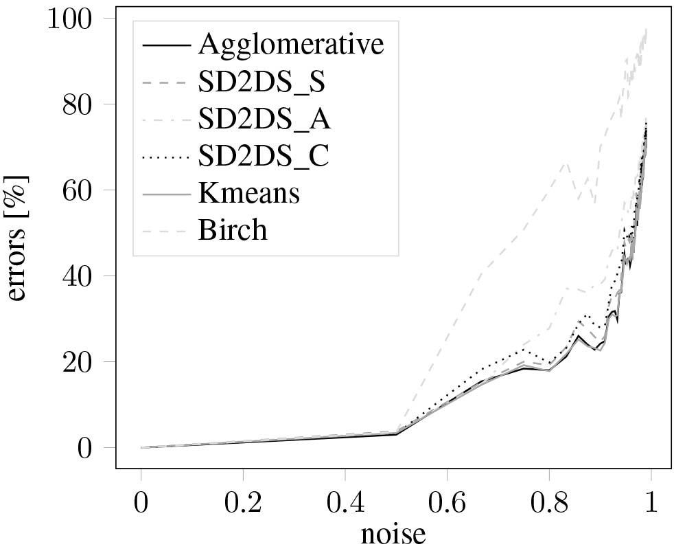
Figure 9.
The classification errors with relation to the data noise for moons clusters.
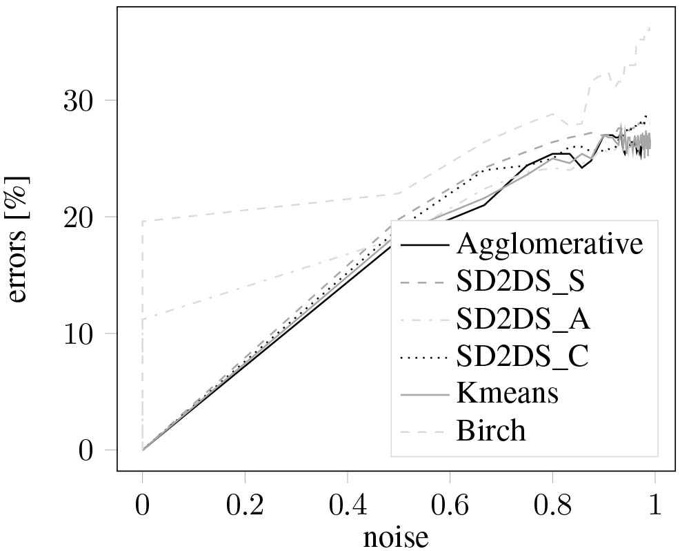
Those two figures prove the good cluster quality results of all the proposed methods. The number of classification errors is strictly similar with both k–means and agglomerative clustering. The slight deterioration introduced by SD2DS_A technique was compensated by using SD2DS_C method. Definitively the worst results were acquired for the birch method which does not perform very well with fixed number of clusters.
Figure 10 presents the results of clustering errors with the relation to the LH* level. All the compared methods present similar results and indicate an improvement of a clustering results with the LH* level growth. Figure 10 also shows that the low value of a threshold in SD2DS_C can give better results.
Figure 10.
The classification errors with relation to the LH* level.
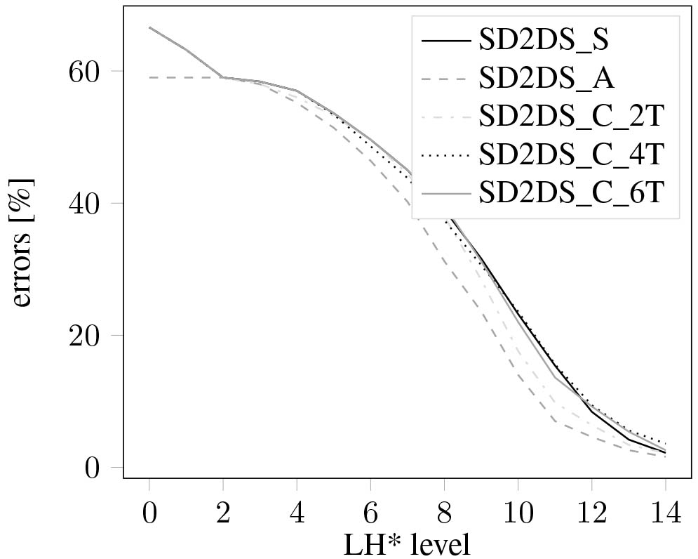
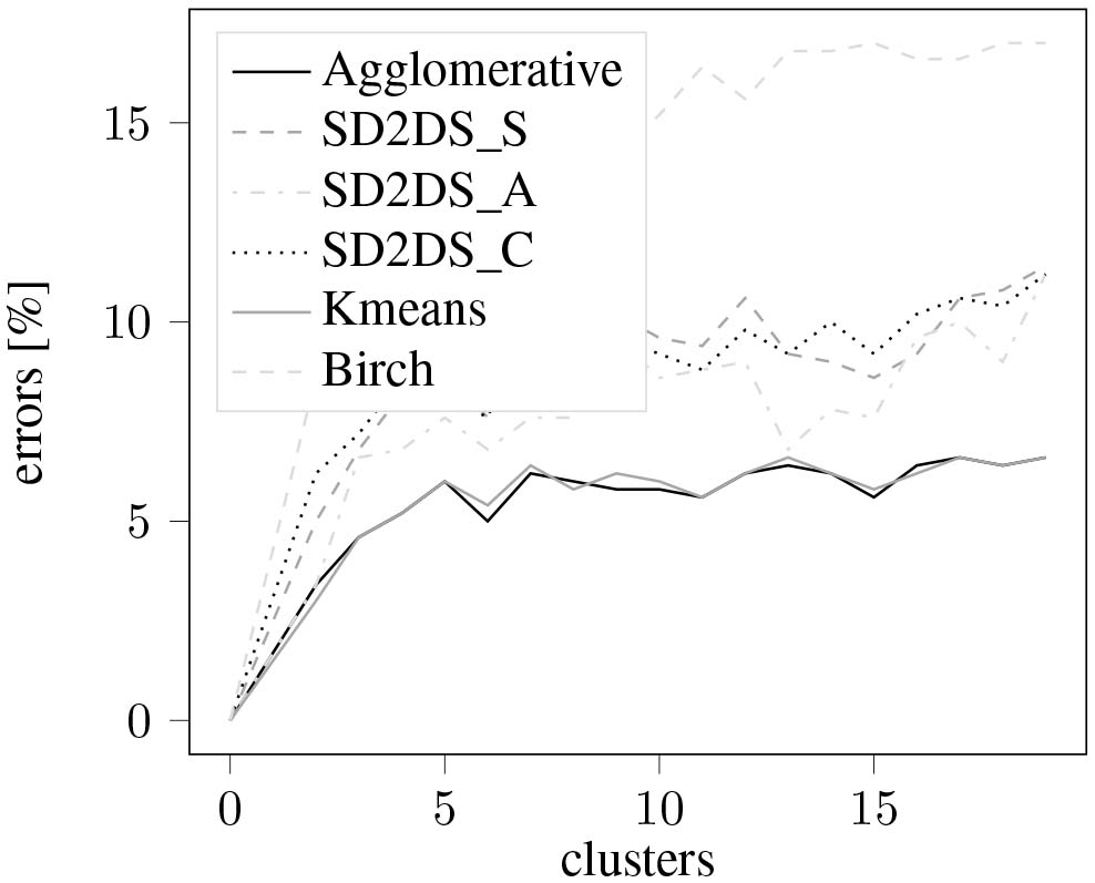
Figure 11 presents the results of clustering errors with the relation to the number of data items. In this figure SD2DS_C_2T, SD2DS_C_4T, SD2DS_C_6T means combined static clustering with threshold set to 2, 4, and 6 respectively. In this case the SD2DS_A generates quite similar results to the k-means and agglomerative clustering which seem to be the most accurate. However, all proposed static clustering techniques seem to be better than birch clustering. The similar conclusions may be drawn from the Fig. 12 in which the clustering errors were evaluated in the relation to the number of clusters.
Figure 11.
The classification errors with relation to the number of data items.
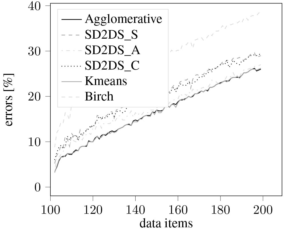
Figure 12.
The classification errors with relation to the number of the clusters.
The evaluation of clustering errors in relation to the number of data features was presented in Figs 13 and 14 with a different data cluster noises (0.5 and 0.9 respectively). As it can be seen for high-dimensional data, the SD2DS_S appears to be the most accurate.
Figure 13.
The classification errors with relation to the number of features (noise
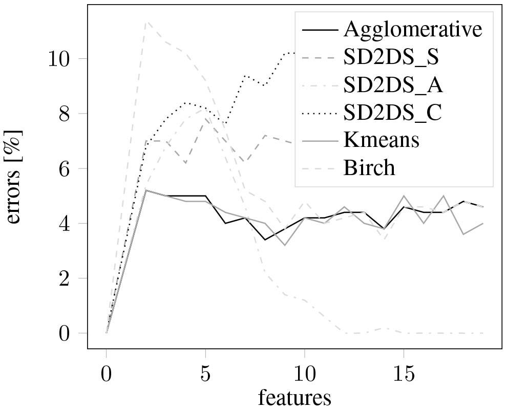
Figure 14.
The classification errors with relation to the number of features (noise

5.2Performance evaluation
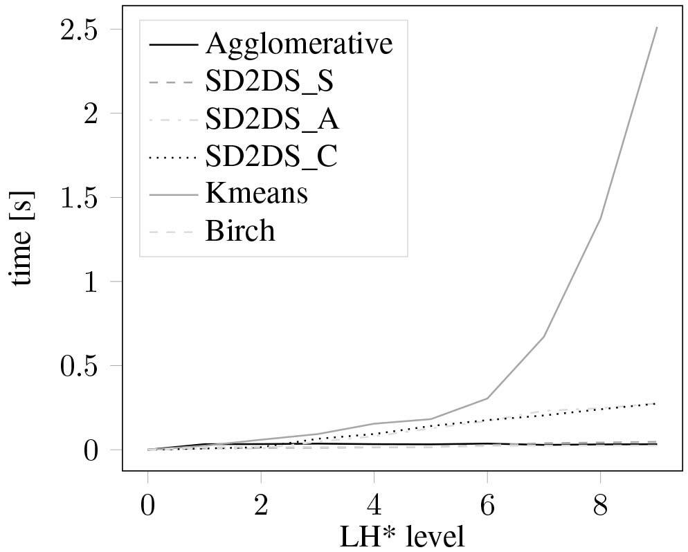
Performance evaluation was carried out by comparing the speed of clustering of a scikit-learn test data set. The speed of clustering with relation to the number of features was presented in Fig. 15. As it can be seen, all proposed algorithms perform faster than traditional k-means technique, however, slower than birch and agglomerative clustering. The evaluation of a clustering speed with relation to the number of data items was presented in Fig. 16. In that case, as the data set grows, the efficiency of a traditional hierarchical, agglomerative method significantly decreases. All the proposed algorithms have much better efficiency than the traditional methods. Similar results were obtained during the evaluation of a speed of clustering with relation to the LH* level. The corresponding result was presented in Fig. 17. In that case the LH* level was correlated with the number of clusters in a form of:
(16)
Figure 15.
The speed of clustering with relation to the number of features.
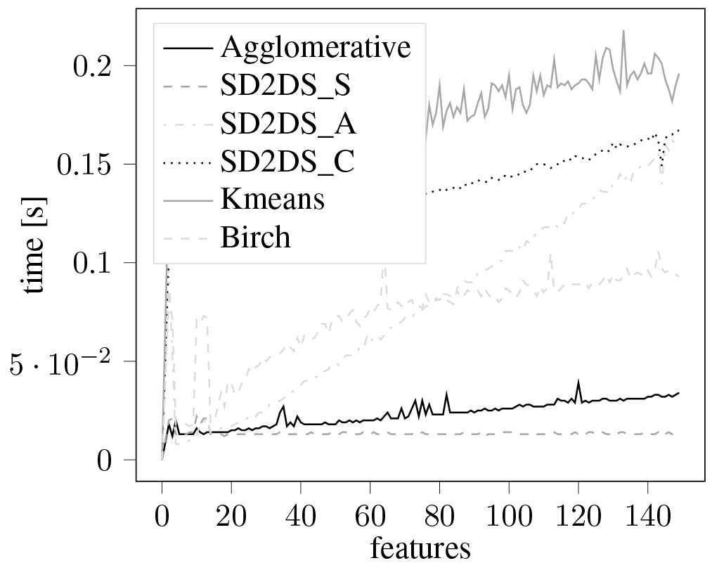
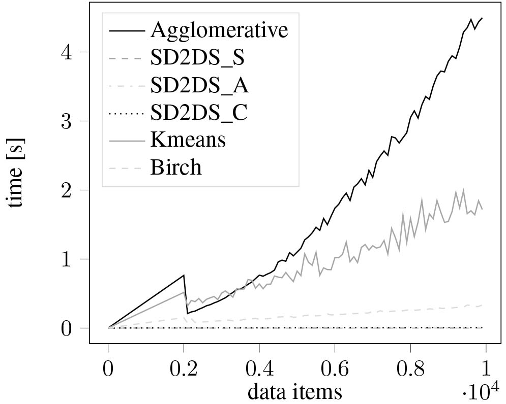
Figure 16.
The speed of clustering with relation to the number of data items.
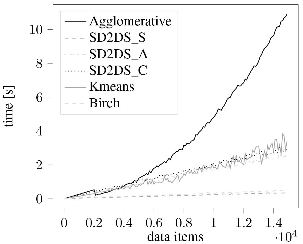
Figure 17.
The speed of clustering with relation to the LH* level.
The next experiment was conducted to evaluate the scalability of all proposed methods. The results were presented in Fig. 18. In the case of inserting additional data item, all the evaluated traditional methods need to process the whole data set to perform clustering. To the contrary, all proposed static clustering techniques allow incremental clustering which can produce almost constant processing time during insertion of additional data items. This is a very important issue for applications with high velocity and volume of the data.
Figure 18.
The scalability of clustering speed with relation to the data items.
5.3Data distribution evaluation
Typical addressing methods in Big Data systems offer a very good data distribution in such a way that all nodes manage a very similar number of data items. This is not the case when the data are distributed based on their content. To measure the quality of data items distribution popular clustering data sets were used from the Fundamental Clustering Problems Suite [41] called LSUN and ATOM.
Figure 19 presents the number of data items that is managed by buckets with different
Figure 19.
Distribution of data items on buckets using LSUN dataset.
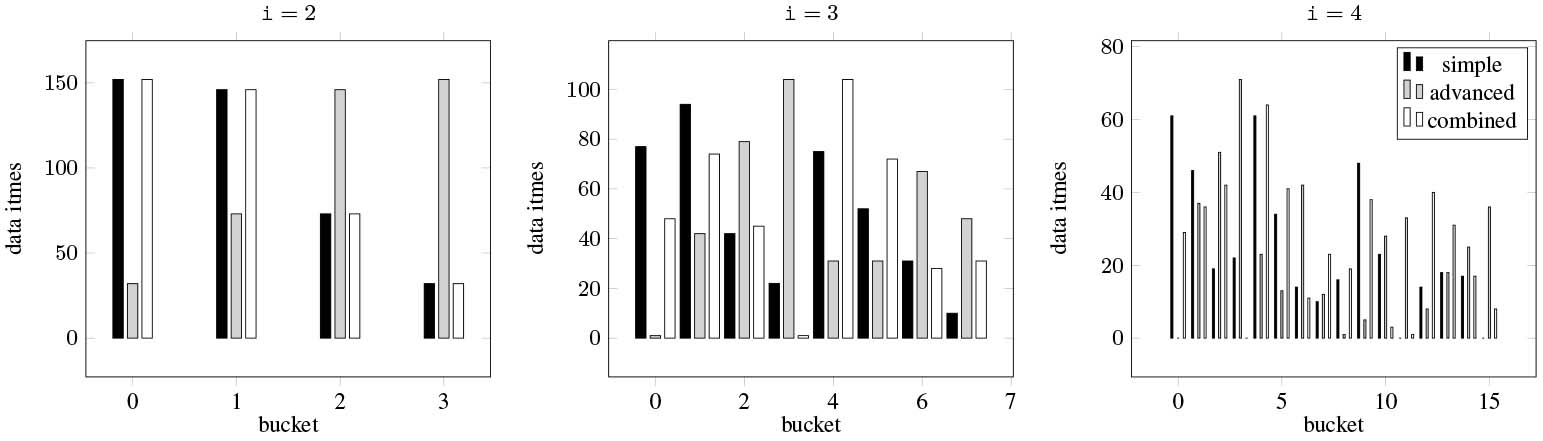
Figure 20.
Standard deviation of bucket load using LSUN dataset.
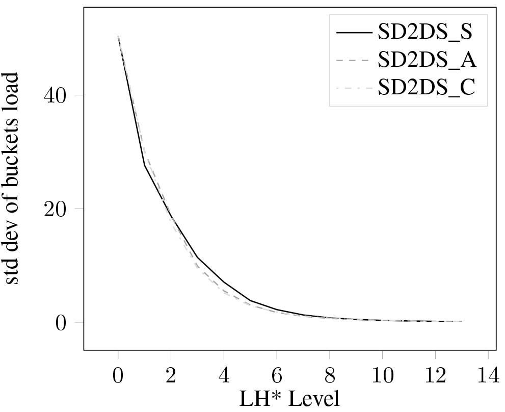
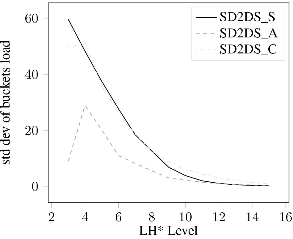
Figure 21.
Standard deviation of bucket load using ATOM dataset.
5.4Big Data evaluation
The most important evaluation was performed on distributed SD2DS implementation on a set of 16 cluster nodes. Additionally, 10 more nodes were used to run clients applications which execute search queries on datastore. The conducted experiments allow to asses how appropriate distribution can help in speeding up the distributed computation. An ATOM [41] data set was used in those experiments. However, this data set is relatively small for big data applications (only 800 samples). That is why it was decided to duplicate data items in such a way that each node consists of even 300.000 data items. In this way by using 16 nodes, the greatest data set consisting of 4.800.000 samples was generated. Duplication was performed simply by inserting each data sample multiple times. No additional noise or other data transformations were introduced. Since all search jobs find all occurrences of searched sample, this simplification does not pose a serious problem. The experiment consisted of performing tasks of searching of data items. Executed jobs, described as MapReduce tasks, are illustrated in Algorithms 5.4 and 23. The Algorithm 5.4 presents a very simple implementation of data items searching that does not consider the data distribution and assumes that each data item may be located on every node (depicted as Naive in the figures). On the other hand, Algorithm 23 is aware of the data distribution in such a way that the Map job searches for the data items only on those nodes that can actually contain them.
Figure 22.
Search time on 960.000 data items with relation to the number of clients.
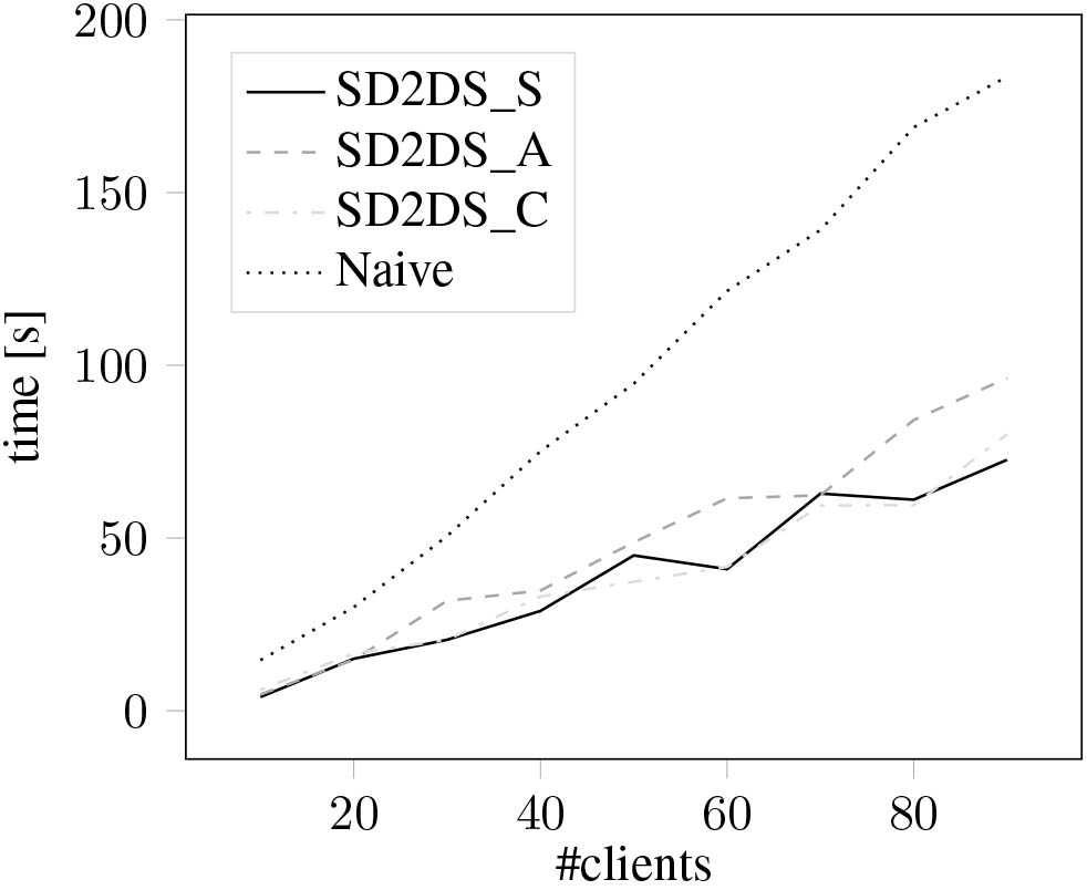
Figure 23.
Search time on 4.800.000 data items with relation to the number of clients.
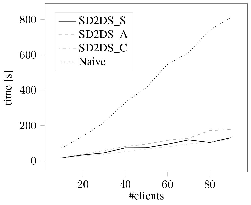
Figures 22 and 23 present comparison of time of searching data items using the proposed distributions with naive approach in a distributed environment with up to 90 clients simultaneously operating on datastorage. Figure 22 presents the result with 960.000 data items stored in the SD2DS while Fig. 23 presents the result with 4.800.000 samples. As it can be seen, the algorithms that are aware of the data items distribution allow to seriously speed up the searching process. All SD2DS specific methods present very similar results while the slowest of them is SD2DS_A method as it is the most computationally expensive.
5.5Discussion
In-depth analysis of all the results allows to draw a conclusion about the comparison of all the proposed methods. In the case of the clustering quality, the proposed SD2DS_A and SD2DS_C methods present the best results, especially with the clusters of complicated shapes. This is especially visible by comparing Figs 8 and 9. Advantages of the quality of the results for the SD2DS_A method are visible when the shapes of the clusters become more and more complicated (i.e. by changing from simple blobs to more complicated moons shapes). However, in the case of the performance the SD2DS_A method appears to be the most time consuming. Previously developed SD2DS_S method is still the fastest one. Since, the scalability of all those methods is very high this performance issue do not pose significant problem.
The ability to deal with arbitrary shape clusters by proposed methods is also visible in the case of the data distribution evaluation. In that case SD2DS_A method is also responsible for generating the best results. In the case of the Big Data evaluation, the difference in performance between SD2DS_S and SD2DS_A method is still visible. As it can be expected, the SD2DS_A is the slowest of all three compared methods.
SD2DS_C method is considered as trade off between the SD2DS_A, time consuming but accurate method, and the fastest SD2DS_S. It allows to increase the quality of the simple method as well as speed up the advanced method. Additionally, a carefully chosen threshold parameter helps to improve the quality result for some problematic clusters (e.g. clusters in the center of the coordinate system).
The most important fact is that all methods present the best quality in terms of the number of errors and data distribution for big values of LH* level. Since the LH* level increases with the overall size of the data set, the quality of the distribution is also strictly correlated with the size of the data.
All proposed methods try to avoid storing dissimilar data items in the same bucket. However, it is possible that similar data items are located on different buckets, especially when the overall number of data items is very high. This should not present a significant problem because a final cluster can be composed from data items from several adjacent buckets. Such buckets, that store similar data items are located very near each other which can be seen for example in Fig. 7.
6.Conclusions
In this paper two new approaches for content aware data items distribution in SD2DS were introduced. The main idea for these methods is to organize the data in the distributed environment and to create an entry point for other data exploration techniques. As it was presented in the paper, the proposed methods are really useful mostly with high-dimensional data. The designed methods allow for creating clusters incrementally which is a great advantage because it does not affect scalability of the datastorage.
It was shown by the experimental results that the two proposed methods (SD2DS_A and SD2DS_C) give better results in terms of clustering quality than previously developed SD2DS_S method. Additionally, those new methods may be considered faster than k-means and agglomerative clustering depending on the nature of the data set (data dimensionality, data item number). All in all, the proposed methods have a very good performance and scalability as well as very similar accuracy to the referenced methods. The combined static clustering (SD2DS_C) appears to be the best methods both in terms of the efficiency and quality compared to the simple static clustering (SD2DS_S) and advanced static clustering (SD2DS_A). Additionally, as it was shown by experiments in real application environment it is possible to create distribution aware algorithms that may seriously speed up the Big Data algorithms. The most important fact is that the accuracy of the proposed methods can be seriously improved with the growth of the whole data set.
As a future work advanced deep learning techniques, like Self Organizing Maps, can be further applied to improve the quality of the static algorithms. It is also possible to verify and improve proposed methods by dynamic clustering methods that run as standard Map Reduce jobs. Dynamic methods will be performed on initially statically partitioned data items, without any additional data transfers, in similar way than using MapReduce, Apache Spark or Apache Kafka. Additionally, the proposed data distribution will be used to develop next efficient Big Data algorithms.
References
[1] | C.C. Aggarwal, S.Y. Philip, J. Han and J. Wang, A framework for clustering evolving data streams, in: Proceedings 2003 VLDB Conference, pages 81–92, Elsevier, (2003) . |
[2] | S. Alam, M. Ata, S. Bailey, F. Beutler, D. Bizyaev, J.A. Blazek, A.S. Bolton, J.R. Brownstein, A. Burden, C.-H. Chuang et al., The clustering of galaxies in the completed sdss-iii baryon oscillation spectroscopic survey: cosmological analysis of the dr12 galaxy sample, Monthly Notices of the Royal Astronomical Society 470: (3) ((2017) ), 2617–2652. |
[3] | R. Altilio, P. Di Lorenzo and M. Panella, Distributed data clustering over networks, Pattern Recognition 93: ((2019) ), 603–620. |
[4] | R. Angles, A comparison of current graph database models, in: 2012 IEEE 28th International Conference on Data Engineering Workshops, pages 171–177, IEEE, (2012) . |
[5] | D. Boley, M. Gini, R. Gross, E.-H.S. Han, K. Hastings, G. Karypis, V. Kumar, B. Mobasher and J. Moore, Partitioning-based clustering for web document categorization, Decision Support Systems 27: (3) ((1999) ), 329–341. |
[6] | A. Bouguettaya, Q. Yu, X. Liu, X. Zhou and A. Song, Efficient agglomerative hierarchical clustering, Expert Systems with Applications 42: (5) ((2015) ), 2785–2797. |
[7] | F. Cao, M. Estert, W. Qian and A. Zhou, Density-based clustering over an evolving data stream with noise, in: Proceedings of the 2006 SIAM International Conference on Data Mining, pages 328–339, SIAM, (2006) . |
[8] | F. Chang, J. Dean, S. Ghemawat, W.C. Hsieh, D.A. Wallach, M. Burrows, T. Chandra, A. Fikes and R.E. Gruber, Bigtable: a distributed storage system for structured data, ACM Transactions on Computer Systems (TOCS) 26: (2) ((2008) ), 1–26. |
[9] | L. Chen, L.-J. Zou and L. Tu, A clustering algorithm for multiple data streams based on spectral component similarity, Information Sciences 183: (1) ((2012) ), 35–47. |
[10] | J. Dean and S. Ghemawat, MapReduce: simplified data processing on large clusters, Communications of the ACM 51: (1) ((2008) ), 107–113. |
[11] | C. Ding, X. He, H. Zha and H.D. Simon, Adaptive dimension reduction for clustering high dimensional data, in: 2002 IEEE International Conference on Data Mining, 2002. Proceedings, pages 147–154, IEEE, (2002) . |
[12] | A. Garg, A. Mangla, N. Gupta and V. Bhatnagar, Pbirch: A scalable parallel clustering algorithm for incremental data, in: 2006 10th International Database Engineering and Applications Symposium (IDEAS’06), pages 315–316, IEEE, (2006) . |
[13] | S. Ghemawat, H. Gobioff and S.-T. Leung, The google file system, in: Proceedings of the Nineteenth ACM Symposium on Operating Systems Principles, pages 29–43, (2003) . |
[14] | K.C. Gowda and G. Krishna, Agglomerative clustering using the concept of mutual nearest neighbourhood, Pattern Recognition 10: (2) ((1978) ), 105–112. |
[15] | J.K. Guest and L.C. Smith Genut, Reducing dimensionality in topology optimization using adaptive design variable fields, International Journal for Numerical Methods in Engineering 81: (8) ((2010) ), 1019–1045. |
[16] | B. Hosseini and K. Kiani, A robust distributed big data clustering-based on adaptive density partitioning using apache spark, Symmetry 10: (8) ((2018) ), 342. |
[17] | S. Hwang, J. Oh, J. Cox, S.J. Tang and H.F. Tibbals, Blood detection in wireless capsule endoscopy using expectation maximization clustering, in: Medical Imaging 2006: Image Processing, Vol. 6144, page 61441P, International Society for Optics and Photonics, (2006) . |
[18] | A.K. Jain, Data clustering: 50 years beyond k-means, Pattern Recognition Letters 31: (8) ((2010) ), 651–666. |
[19] | V. Kalavri and V. Vlassov, Mapreduce: Limitations, optimizations and open issues, in: 2013 12th IEEE International Conference on Trust, Security and Privacy in Computing and Communications, pages 1031–1038, IEEE, (2013) . |
[20] | W. Kim, Parallel clustering algorithms: survey, Parallel Algorithms, Spring 34: ((2009) ), 43. |
[21] | J.M. Kleinberg, An impossibility theorem for clustering, in: Advances in Neural Information Processing Systems, pages 463–470, (2003) . |
[22] | A. Krechowicz, A. Chrobot, S. Deniziak and G. Łukawski, SD2DS-based datastore for large files, in: Federated Conference on Software Development and Object Technologies, pages 150–168, Springer, (2015) . |
[23] | A. Krechowicz and S. Deniziak, Business intelligence platform for big data based on scalable distributed two-layer data store, in: Communication Papers of the 2017 Federated Conference on Computer Science and Information Systems, M. Ganzha, L. Maciaszek, M. Paprzycki (eds). ACSIS, Vol. 13, pages 177–182, (2017) . |
[24] | A. Krechowicz and S. Deniziak, Hierarchical clustering in scalable distributed two-layer datastore for big data as a service, in: 2018 Sixth International Conference on Enterprise Systems (ES), pages 138–145, IEEE, (2018) . |
[25] | A. Krechowicz, S. Deniziak, M. Bedla, A. Chrobot and G. Łukawski, Scalable distributed two-layer block based datastore, in: International Conference on Parallel Processing and Applied Mathematics, pages 302–311, Springer International Publishing, (2015) . |
[26] | Y. Liang, M.-F. Balcan and V. Kanchanapally, Distributed pca and k-means clustering, in: The Big Learning Workshop at NIPS, Vol. 2013, Citeseer, (2013) . |
[27] | W. Litwin, M.-A. Neimat and D.A. Schneider, LH*: Linear Hashing for distributed files, Vol. 22, ACM, (1993) . |
[28] | V. Melnykov and S. Michael, Clustering large datasets by merging k-means solutions, Journal of Classification, pages 1–27, (2019) . |
[29] | J.J. Miller, Graph database applications and concepts with neo4j, in: Proceedings of the Southern Association for Information Systems Conference, Atlanta, GA, USA, Vol. 2324, (2013) . |
[30] | V. Olman, F. Mao, H. Wu and Y. Xu, Parallel clustering algorithm for large data sets with applications in bioinformatics, IEEE/ACM Transactions on Computational Biology and Bioinformatics 6: (2) ((2008) ), 344–352. |
[31] | F. Pedregosa, G. Varoquaux, A. Gramfort, V. Michel, B. Thirion, O. Grisel, M. Blondel, P. Prettenhofer, R. Weiss, V. Dubourg, J. Vanderplas, A. Passos, D. Cournapeau, M. Brucher, M. Perrot and E. Duchesnay, Scikit-learn: machine learning in python, Journal of Machine Learning Research 12: ((2011) ), 2825–2830. |
[32] | E. Plugge, T. Hawkins and P. Membrey, The Definitive Guide to MongoDB: The NoSQL Database for Cloud and Desktop Computing, Apress, Berkely, CA, USA, 1st edition, (2010) . |
[33] | D.G. Reis, F.S. Gasparoni, M. Holanda, M. Victorino, M. Ladeira and E.O. Ribeiro, An evaluation of data model for nosql document-based databases, in: World Conference on Information Systems and Technologies, pages 616–625, Springer, (2018) . |
[34] | R.S. Sangam and H. Om, Equi-clustream: a framework for clustering time evolving mixed data, Advances in Data Analysis and Classification 12: (4) ((2018) ), 973–995. |
[35] | P. Shrivastava, L. Sahoo, M. Pandey and S. Agrawal, Akm-augmentation of k-means clustering algorithm for big data, in: Intelligent Engineering Informatics, pages 103–109, Springer, (2018) . |
[36] | K. Shvachko, H. Kuang, S. Radia and R. Chansler, The hadoop distributed file system, in: 2010 IEEE 26th Symposium on Mass Storage Systems and Technologies (MSST), pages 1–10, Ieee, (2010) . |
[37] | S. Sivasubramanian, Amazon dynamodb: a seamlessly scalable non-relational database service, in: Proceedings of the 2012 ACM SIGMOD International Conference on Management of Data, pages 729–730, (2012) . |
[38] | C. Strauch, U.-L.S. Sites and W. Kriha, Nosql databases, Lecture Notes, Stuttgart Media University 20: ((2011) ), 24. |
[39] | Z. Sun, G. Fox, W. Gu and Z. Li, A parallel clustering method combined information bottleneck theory and centroid-based clustering, The Journal of Supercomputing 69: (1) ((2014) ), 452–467. |
[40] | K.M.M. Thein, Apache kafka: next generation distributed messaging system, International Journal of Scientific Engineering and Technology Research 3: (47) ((2014) ), 9478–9483. |
[41] | A. Ultsch, Fundamental clustering problems suite (fcps), Technical report, Technical report, University of Marburg, (2005) . |
[42] | J. Vesanto and E. Alhoniemi, Clustering of the self-organizing map, IEEE Transactions on Neural Networks 11: (3) ((2000) ), 586–600. |
[43] | M.N. Vora, Hadoop-hbase for large-scale data, in: Proceedings of 2011 International Conference on Computer Science and Network Technology, Vol. 1, pages 601–605, IEEE, (2011) . |
[44] | X. Xu, J. Jäger and H.-P. Kriegel, A fast parallel clustering algorithm for large spatial databases, in: High Performance Data Mining, pages 263–290, Springer, (1999) . |
[45] | X. Yang and J. Sun, An analytical performance model of mapreduce, in: 2011 IEEE International Conference on Cloud Computing and Intelligence Systems, pages 306–310, IEEE, (2011) . |
[46] | M. Zaharia, R.S. Xin, P. Wendell, T. Das, M. Armbrust, A. Dave, X. Meng, J. Rosen, S. Venkataraman, M.J. Franklin et al., Apache spark: a unified engine for big data processing, Communications of the ACM 59: (11) ((2016) ), 56–65. |
[47] | T. Zhang, R. Ramakrishnan and M. Livny, Birch: an efficient data clustering method for very large databases, in: ACM Sigmod Record, Vol. 25, pages 103–114, ACM, (1996) . |
[48] | W. Zhao, H. Ma and Q. He, Parallel k-means clustering based on mapreduce, in: IEEE International Conference on Cloud Computing, pages 674–679, Springer, (2009) . |
[49] | A. Zhou, F. Cao, W. Qian and C. Jin, Tracking clusters in evolving data streams over sliding windows, Knowledge and Information Systems 15: (2) ((2008) ), 181–214. |


