
Efficient surface defect detection in industrial screen printing with minimized labeling effort
Abstract
As part of the evolving Industry 4.0 landscape, machine learning-based visual inspection plays a key role in enhancing production efficiency. Screen printing, a versatile and cost-effective manufacturing technique, is widely applied in industries like electronics, textiles, and automotive. However, the production of complex multilayered designs is error-prone, resulting in a variety of defect appearances and classes. These defects can be characterized as small in relation to large sample areas and weakly pronounced. Sufficient defect visualization and robust defect detection methods are essential to address these challenges, especially considering the permitted design variability. In this work, we present a novel automatic visual inspection system for surface defect detection on decorated foil plates. Customized optical modalities, integrated into a sequential inspection procedure, enable defect visualization of production-related defect classes. The introduced patch-wise defect detection methods, designed to leverage less labeled data, prove effective for industrial defect detection, meeting the given process requirements. In this context, we propose an industry-applicable and scalable data preprocessing workflow that minimizes the overall labeling effort while maintaining high detection performance, as known in supervised settings. Moreover, the presented methods, not relying on any labeled defective training data, outperformed a state-of-the-art unsupervised anomaly detection method in terms of defect detection performance and inference speed.
1.Introduction
Visual quality inspection plays a key role in achieving quality standards of premium manufacturers. As even the smallest defects in high-quality components lead to customer complaints, zero-defect policies are striven, resulting in visual inspection of every produced part. According to the manufacturing industry and the underlying production processes, manual visual inspection is still common. Therefore, huge amounts of human resources are required, conducting elaborate workflows accompanied with monotonous visual inspection tasks. This results in overlooked defects as well as unnecessary rejects of produced parts according to the subjective assessment of the operator [1]. In order to reduce these quality fluctuations and thus improve competitiveness, the automation of quality inspection processes as part of the emerging Industry 4.0 is mandatory [2, 3, 4, 5]. Thus, machine learning-based visual inspection systems [6, 7, 8] are intensively researched and build a crucial part for ensuring 100% fault-free products. High demand for automated visual inspection arises in the electronics industries [9]. Common inspected components include LEDs, semiconductor wafers and printed circuit boards [10]. In addition to electronics, there is high demand in the textile [11, 12, 13], printing [14, 15, 16] and automotive industries [17, 18]. Automatic visual inspection systems can be applied to almost all materials such as polymers, metals, ceramics, glass, etc., regardless of the industry.
1.1Machine vision inspection process
In general, machine vision inspection can be roughly divided into three main stages: defect visualization, preprocessing, and inference. Based on the optical surface properties of the sample under investigation, appropriate optical components must be determined. These components include cameras (sensors incl. optics), illuminations, and filters, which are used to visualize defects and reduce the prominence of unimportant features. Thus, the objective of defect visualization is to maximize the contrast of imperfections on product surfaces in digital images, making them more easily identifiable and analyzable. Determining suitable optical components typically requires extensive laboratory experiments and domain knowledge. General approaches for automatically characterizing defect visibility, applicable to various surfaces and defect textures, remain an active area of research [19, 20, 21].
In addition to the common RGB and monochrome sensors in the visible range, sensors operating in the ultraviolet (UV) or infrared (IR) ranges can offer advantages for specific features. For instance, UV sensors (200–400 nm) reveal fine scratches on polished surfaces that are barely visible to the human eye (e.g. Sony’s IMX487 [22]). Shortwave infrared (SWIR) sensors (900–1700 nm) are increasingly applied in the electronics and semiconductor industries to uncover subsurface defects [23]. Multi- or hyperspectral cameras, which combine different spectral bands (e.g. visible and IR), reveal spatial physical and chemical properties of the samples being examined [24, 25]. These imaging techniques are particularly valuable in the food, waste management, packaging, agricultural, and pharmaceutical sectors [26, 27]. However, exploiting additional spectral bands is accompanied by an increased workload for data processing. Besides the selected spectrum, the optimal optical modality is determined by the illumination conditions, including the illumination characteristics (e.g. direct, diffuse, structured) and its position relative to the surface and sensor (bright field, dark field or transmission).
In addition to the defect visualization capabilities, factors such as system integration complexity, data processing bandwidth and software interoperability, are crucial in selecting appropriate hardware for industrial applications.
Image preprocessing prepares the captured data for inference with the selected defect detection methods. This stage may involve tasks such as image registration, masking, resizing or data normalization, to name a few. Finally, inference is used for the decision-making, classifying the inspected product as normal or defective.
1.2Industrial defect detection methods
With the rise of affordable computing power, deep learning-based research has gained significant momentum in machine vision tasks. Deep convolutional neural networks (DCNN) have shown superior performance over traditional defect detection methods that rely on manual feature engineering [28]. The performance of deep learning methods typically scales with the amount of available training data. However, collecting large quantities of labeled data is labor-intensive and often impractical for many industrial applications. In the context of surface defect inspection using supervised neural networks, this is a major limitation, as an extensive labeling process is required for each new product type to meet inspection standards. Consequently, current research focuses on semi- or unsupervised defect detection methods [29, 30], which require minimal or no defective samples for training and are therefore of particular interest for industrial applications. By modeling the underlying data distribution of fault-free (normal) samples, unsupervised methods overcome possible generalization problems of supervised methods.
Since the publication of industrial defect detection datasets such as MVTec [31], several anomaly detection methods have emerged. These unsupervised methods can be broadly categorized into representation-based [32, 33, 34, 35], generative model-based [36, 37, 38, 39, 40, 41, 42], and flow-based [43, 44] approaches. Representation-based methods compare test data features with learned normal representations to measure feature similarity or distance. Flow-based methods map feature distributions to multivariate Gaussian distributions using normalizing flows, with deviations indicating anomalies. Both approaches use DCNN feature extractors pretrained on large datasets like ImageNet [45]. These methods are often memory and computationally intensive due to their architectures and algorithms, such as k-nearest neighbor. Furthermore, the feature extractors are biased towards the dataset used for pre-training, which leads to performance degradation in case of significantly different examined data distributions.
Generative models are designed to reconstruct normal data, failing to properly reconstruct defective regions resulting in anomaly scores. Despite progress with autoencoders [36], generative adversarial networks (GANs) [46, 38, 39] and denoising diffusion models [40, 41, 42], challenges persist in overcoming reconstruction limitations for fine-grained patterns as well as computational efficiency.
Additional approaches include synthesizing defective data samples for self-supervised pretraining or data augmentation [47, 48, 49, 50, 51]. However, GAN-based synthetization tends to generate simple defect structures and struggles with complex patterns. In addition, these methods rely on large datasets including defective samples for the initial training process. Recent research on few-shot generative models, including diffusion-based approaches, aims to address these issues [52, 53, 54, 55].
Given the specific data distributions and detection tasks in industrial applications, specialized methods are crucial. The high permissible variability in complex design patterns of screen-printed products and their diverse product portfolio demands robust and adaptable methods. In addition, short inference times are mandatory in order to achieve the required process cycle times.
1.3Related work
Ongoing research on defect detection of screen-printed products is being increasingly applied in the electronics industry. In Zhao et al. [56], the screen-print of batteries is inspected using a multi-level block template matching and k-nearest neighbor method. The presented inspection system enables the detection of defects, such as blurred prints, local defects or scratches of the printed product logo, QR code and fabrication number. Further work presents an automatic inspection system for surface defect detection of screen-printed mobile phone back glasses [57]. A dual brightfield imaging system is demonstrated for defect visualization. It consists of a coaxial bright field and a low angle bright field illumination, enabling the visualization of defects such as scratches, dents and discolorations. Defect detection was performed with a symmetric semantic segmentation network trained in a supervised manner. The training dataset consisted of 34 550 images (6742 defectives), achieving an average test precision and recall of 91.8 and 95.3%. Another inspection solution for mobile phone cover glasses is presented in [58]. The system adopts backlight imaging in combination with a segmentation method trained in an adversarial manner utilizing a novel data generation process. A further defect detection method applied to a screen-printing process is based on an optimized U-Net++ [59] architecture, which is described in [60]. To enable accurate detection of small defects in relation to the product size, only image patches were evaluated rather than the entire image. The visualization of the defects was done with a white backlight and a blue incident illumination. Using the patch-split method and a customized loss function, a dice score of 0.73 was achieved. Gafurov et al. [61] investigated smearing effects of screen-printed lines using deep neural networks (DNN) and CCD cameras, installed subsequent to the screen-printing process. For this purpose, a screen-printing mask was designed containing different line widths and spacings as well as a variation of squeegee directions. Using an adapted U-Net architecture, it was possible to detect smearing defects in various printing conditions.
Commercially available automatic visual inspection systems are known in the printing, glass and weaving industries [62, 63, 64, 65, 66, 67, 68, 69, 70]. However, inspection solutions for defect detection in the field of screen-printing are rather limited. The company OMSO [71] offers a product for optical inspection of decorations on cylindrically shaped objects such as bottles, tubes and jars. Cugher’s glass inspection system [72] enables the detection of defects on the screen-print designs of glass panels. Keko Equipment Ltd. [73] offers an automatic inspection system to inspect prints on multilayer green ceramic productions. The inspection software leverages e.g. golden template comparison applicable for max. inspection areas of 220
1.4Contributions
The aforementioned studies and commercial automated inspection systems mostly contain inspection solutions for printed product designs such as logos and labels, showing clearly defined geometries and image features. Due to non-complex print designs, e.g. by using only a few print layers, the spectrum of possible defect causes and subsequent diverse defect appearances is reduced, which limits the effort of defect visualization. Frequently used deep learning-based segmentation models rely on pixel-wise labeled ground truth masks for supervised training and are therefore dependent on the amount and quality of labeled data.
The products studied for the given publication are designed for use as decorative patterns in a variety of applications, including products used in the automotive industry. In order to meet the customer’s needs and requirements, complex designs are developed and manufactured under high quality standards. To achieve the desired visual impression of the decorative pattern, numerous manufacturing steps are necessary, resulting in a complex multilayered design. Therefore, the aim of this work was to develop an automatic visual inspection system that inspects decorated foil plates for production-related surface defects. Generally, the defects appear small in relation to the sample size being examined. The developed optical modalities must be able to display the different defect classes with sufficient contrast. Given the large product portfolio, the adaptability of the system to new product designs is of great importance. In addition, the applicability of automated visual inspection in the production line should be ensured with regard to important process requirements such as cycle times. Due to the high labor involved in data acquisition and labeling, defect detection methods that provide sufficient detection performance with as little labeling effort as possible are emphasized. Furthermore, they must be capable of handling the allowed product to product variability.
Currently, there is no available inspection system for automated full-surface defect detection of decorated foil plates, accounting for allowed design and product variability and adaptability. It has to be mentioned that this publication builds upon the research work presented at the ASPAI 2022 [75]. Optical modalities were introduced that enable the visualization of production-related defects with sufficient contrast. Therefore, laboratory experiments were conducted to analyze various design patterns of different products. The possible integration of investigated optical modalities into the production line as part of an inspection approach was outlined. By assigning the detected defect classes to the individual production steps, deviations in the production process will be detected at an early stage.
Thus, the main contributions of this work can be summarized as follows:
• Investigation and application of developed optical modalities for sufficient defect visualization in a sequential inspection process, given production related requirements. This includes adaptability to different product sizes with a “field of view” (FOV) of up to 1200 mm, as well as to product designs with their various defect appearances and resulting defect classes.
• Introduction of scalable patch-wise defect detection methods utilizing less labeled data, applicable for automatic full-surface defect detection. Therefore, a data preparation and preprocessing workflow is presented, that minimizes the overall labeling effort in supervised training settings, applicable to various industrial manufacturing processes. This enables fast adaptability as allowable product-to-product variations and unseen defect types during production emerge.
• Development and implementation of an inspection system demonstrator in an industrial setting, capable of automatic defect detection on decorated foil plates.
Section 2 illustrates the structure of decorated foil plates and briefly describes the manufacturing process. Frequently occurring defects are visualized and the formation process of selected ones is described. In Section 3 experimentally explored optical modalities are specified, followed by an introduction of the inspection system and its underlying procedures in Section 4. Section 5 presents the investigated defect detection methods. Section 6 gives an evaluation of their defect detection performance as well as inference speed and overall inspection time. Section 7 provides a summary of the key findings and an outlook for future improvements.
2.Decorated foil plate
The manufacturing process underlying the products studied is known as screen printing or silk screen printing. This is a cost-effective and versatile printing process that can be applied to a wide range of different materials such as textiles, metals, glass, wood and polymers [76]. The process is suitable for automation and is widely used in industries such as textiles, automotive and electronics [77]. Thereby, ink is deposited on the sample through a screen with a defined design. The screen consists of a frame with close-meshed fibers, forming a grid, onto which a UV-active photo emulsion is evenly applied. Once the emulsion has dried, the desired design is transferred to the screen using a film exposed to a UV light source. Areas that have not been exposed to UV light are then washed out and are permeable to the ink. In the subsequent printing process, the ink is transferred through the created stencil to the underlying sample. The sequential repetition of these production steps using separate screens for each ink layer enables the production of multilayer decorative patterns. The correct alignment of the individual layers to each other and the quality of each production step have an influence on the final print result.
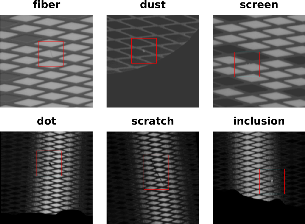
Figure 1.
Schematic multilayered design of a decorated foil plate showing possible defective (red) and fault-free patches (blue). Defects appear small (few pixels in extension) in relation to the investigated sample size of up to 106 mm2.
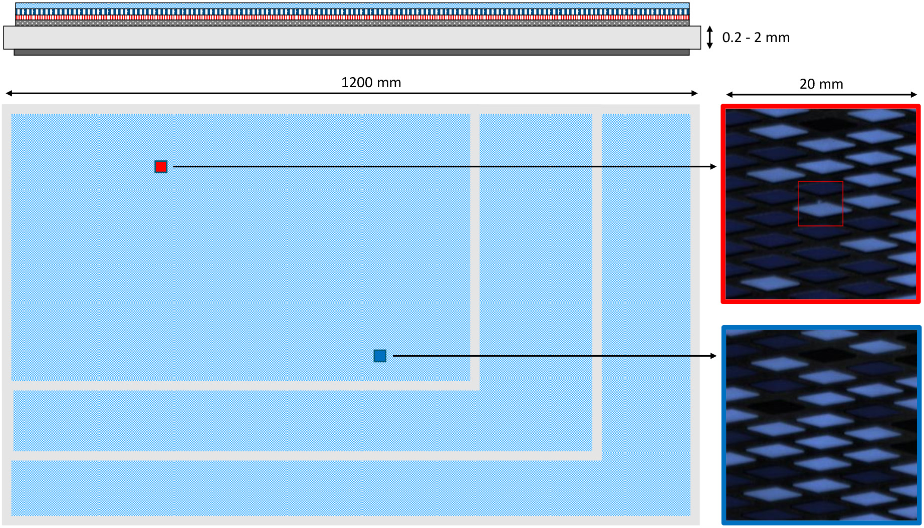
Figure 1 schematically shows a typical structure of a decorated foil plate. Depending on the product design the dimensions of the carrier foil vary from A4 format to a width of 1200 mm. Typical materials are polymers such as polycarbonate (PC), poly(methyl methacrylate) (PMMA), acrylonitrile butadiene styrene (ABS), polyethylene terephthalate (PET) or polyvinyl chloride (PVC). The decorative pattern is formed by sequentially depositing ink layers on the front- and/or backside of the carrier foil. The customized screens determine the design as well as the possible print resolution, which is defined by the number of meshes per inch and the ratio of thread diameter to mesh opening [78]. Depending on the complexity of the decorative design, more than 10 different colored layers are applied. As a result, high-quality appealing decorative patterns are obtained, which in some applications can yield a visual 3D effect.
2.1Defect formation process and defect classes
The complex manufacturing process results in a large number of possible defect causes. Basically, defects can occur in every manufacturing step, which cumulatively affect the final product. Understanding the origin of defects and their visual appearance is of central importance for optimizing the quality standards in the manufacturing processes and, in the event of their occurrence, for taking corrective action. In this work, possible process-related surface defects are investigated. In the case of surface defect detection, a defect can be generally described as any sufficient deviation from the normal sample, considering the allowable product variability. Typical defect classes include e.g. printing defects, inclusions, mechanical deformations, scratches, smears, squeegee strokes, pinholes, dust and misregistered control markers. On the right side of Fig. 1, two image patches on a structured decorative pattern are illustrated. The defects appear small (approx. 0.07 mm2 on the upper right defective patch), i.e. only a few pixels in size, relative to the product size of up to 106 mm2. A further characteristic is the high permissible design variability of the structured patterns. This is evident when comparing the variance in contrasts of the patches mentioned above. Depending on the location of occurrence and product design, these defects can also be defined as weakly contrasted.
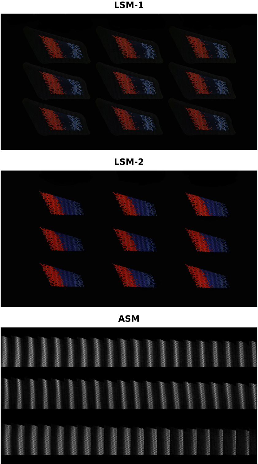
Figure 2.
Visualized defective patches of selected production-related defect classes captured by means of the customized optical modalities. Each row corresponds to a modality, from top to bottom: Line Scan Modality 1, Line Scan Modality 2, Area Scan Modality. Depending on their spatial appearance, defects can be divided into point defects such as inclusions (1A), screen or print defects (1B), scratches or dots (3A/3B) and pinholes (2A), or area defects such as pattern misalignment (1C/2C), inhomogeneities (2B) or squeegee strokes (3C).
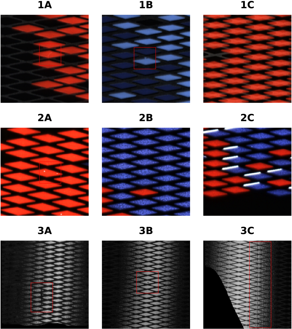
Figure 3.
Relative positioning of the camera sensors and illuminations regarding the utilized optical modalities: Line Scan Modality 1 (LSM-1), Line Scan Modality 2 (LSM-2) and Area Scan Modality (ASM), as presented at the ASPAI 2022 [75].
![Relative positioning of the camera sensors and illuminations regarding the utilized optical modalities: Line Scan Modality 1 (LSM-1), Line Scan Modality 2 (LSM-2) and Area Scan Modality (ASM), as presented at the ASPAI 2022 [75].](https://content.iospress.com:443/media/ica/2025/32-1/ica-32-1-ica240742/ica-32-ica240742-g003.jpg)
Prior to each print cycle, the new print layer is precisely aligned to the existing layers. Any misalignment of individual print layers during this registration process will be visible in the printed pattern by a so-called pattern misalignment, which is apparent across the entire surface (Fig. 2, 1C/2C). Deviations during the ink application process, e.g. regions with too less ink application, lead to pinholes or inhomogeneities (Fig. 2, 2A/2B). Inhomogeneities are print layers with too low optical density and high variance in color values. Pinholes, in turn, appear as dot-shaped holes in the print pattern. Impermissible holes or closed meshes in the stencil of the screen can lead to screen and print defects (Fig. 2, 1B). Typical inclusions in individual ink layers, such as dust and fibers (Fig. 2, 1A), are caused by impurities in the process environment and electrostatic charge on the foil plates. Due to an electrostatic interaction with charged particles in certain inks, static splashes or stains may also occur. Automatic or manual product handling can cause scratches or dots (Fig. 2, 3A/3B), as well as two-dimensional mechanical deformations, within the topcoat layer. Changes in the uniformity of the squeegee pressure and the dwell time of the ink on the screen can lead to a variable ink application. These so-called squeegee strokes (Fig. 2, 3C) are characterized as area defects and are affected by the printing direction.
3.Defect visualization
Defect visualization with sufficient contrast forms the basis of surface defect detection. Due to the characteristic design of decorated foil plates, a large number of defect classes emerge, which only become visible using certain optical modalities. In addition, some defect classes only occur in distinct decorative patterns. To find the best possible optical modalities, optical experiments were performed on a variety of decorative patterns and designs. According to the compliance standards of the project partner, however, only images of a selected decorative pattern are illustrated in the given publication. The experiments included different sensor designs (area, line sensor) as well as illumination techniques (brightfield, darkfield, and transmission) in the visible range. As presented in [75] it turned out that three different optical modalities are necessary to visualize the wide range of defect classes. The optical modalities: Line Scan Modality 1 (LSM-1), Line Scan Modality 2 (LSM-2) and Area Scan Modality (ASM), consisting of camera and illumination as well as their positioning in relation to each other, are schematically visualized in Fig. 3.
3.1Line scan modality 1
LSM-1 consists of an RGB linescan camera and a high intensity LED line bar (white, 6200 K). The illumination is equipped with a special lens and light amplifier foil to ensure the most directional and brightest illumination in the focal zone. The optimum distance, determined by the optical characteristics of the line bar, is approximately 50 mm above the sample’s surface. The relative arrangement of light source and camera, enable a dark field illumination. The camera is placed planar to the sample’s surface and the angle of incidence of the illumination is chosen as steep as possible w.r.t. the horizontal plane. This positioning avoids strong shadowing in complex decorative patterns showing a 3D effect. Patches 1A–1C in Fig. 2 were recorded by means of this setup. Small punctual defects such as screen defects or inclusions that stand out only slightly from the background, are displayed in good contrast. Furthermore, area defects such as the pattern misalignment of an entire print layer, occurring as semitransparent white overlay in patch 1C, is clearly pronounced. This setup is applicable for defects affecting the decorated pattern like slurred prints. In addition, it addresses “sawtooth” defects, defined as continuous eroding at patterned edges, as well as misregistered control markers.
3.2Line scan modality 2
LSM-2 similarly utilizes an RGB line scan camera and a high intensity LED line bar. The illumination is placed planar and opposite to the camera aligned to its optical axis. As shown in Fig. 3, this setup allows transmission measurements of the investigated sample. As in LSM-1, the optimal distance is determined by the optical characteristics of the line bar (approx. 50 mm behind the sample) to achieve the highest possible illumination intensity. A planar alignment of sensor and illumination to the sample’s surface is mandatory to reliably investigate thicker layers on large-sized samples, mitigating geometrical influences on the optical path. As in the LSM-1 setup, the camera distance is determined by the demanded maximum FOV as well as the required object pixel size and can be greater than 1000 mm dependent on the sensor design. In addition to defects such as pinholes or pattern misalignment (Fig. 2, 2A/2C), it is also possible to display unwanted inhomogeneities in semitransparent colored print layers (Fig. 2, 2B). Line scan cameras in combination with high intensity line bars are generally the appropriate choice for the dynamic inspection of flat surfaces, as they are capable of capturing high resolution images at high measurement speeds, regardless of the sample size in the transport direction. However, the experiments conducted with the line scan camera revealed that the detection of defects on the transparent top layer was not satisfactory.
3.3Area scan modality
To overcome above mentioned limitations an optical modality, consisting of an area scan camera and a light bar aligned in direct reflection, was designed (ASM in Fig. 3). Therefore, the LED light bar (white, 6200 K) is placed as far away as possible from the specimen’s surface to create a large optical lever with respect to the monochromatic camera sensor. As shown in Fig. 2 3A–3C, this illumination method produces a bright area of direct reflection in the center, which decreases and fades out to the margins. Defects such as squeegee strokes or smears are only visible with high contrast in this transition area of reflection (Fig. 2, 3C). In general, bright-field images differ significantly from dark-field images in the LSM-1 and reveal defects in the transparent top layer, such as scratches and mechanical deformations (Fig. 2, 3A/3B). The majority of defects in the transparent top layer are only visible using this modality.
Utilizing all three modalities it was feasible to visualize the required production-related defect classes with sufficient contrast within the range of a few pixels in extension and minimum object pixel sizes of approx. 75
4.Inspection system
The optical modalities enable a visualization of the production-specific defect classes with sufficient contrast. In order to perform an automatic visual product inspection using these modalities, an inspection system demonstrator was designed and installed at the project partner’s production facility. The following main system requirements were considered: 1) Maximum product inspection time is determined by the conveyor speed and transport length and ranges between 15–30 s. 2) Product sizes of up to 1200 mm (FOV) should be examinable. 3) Adaptivity to different products and designs must be provided. 4) The defect detection methods must be able to detect smallest defects in relation to product sizes considering the allowed product to product variations. Furthermore, little efforts in data labeling as well as inference speeds applicable for in-line inspection are demanded.
Figure 4.
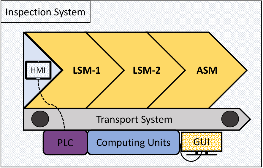
Main components of the inspection system demonstrator, installed at the production site: Measurement chambers as LSM-1, LSM-2 and ASM; Programmable Logic Controller as PLC; Human Machine Interface as HMI; Graphical User Interface as GUI.
4.1Inspection procedure
As shown in Fig. 4, the inspection system demonstrator consists of three measurement chambers, respectively one for each modality LSM-1, LSM-2 and ASM, which are arranged in sequence. Each measurement chamber is optically shielded to avoid both ambient light and unwanted reflections from different chambers. Regarding the above stated system requirements as well as required optical modalities, suitable hardware components had to be selected. The hardware components of the measurement chamber LSM-1 and LSM-2 consist of commercial 16k RGB line scan cameras including optics and commercial high-power LED line bars according to Section 3. Due to the large required FOV of 1200 mm, 4 side by side monochrome area scan cameras (2.2 MP) incl. optics in combination with a high-power bar light are mounted in ASM. During each measurement cycle, the sample is manually placed on a conveyor belt and sequentially transported through all three measurement chambers. An installed rotary encoder generates trigger signals that enable distortion-free image acquisition at different conveyor speeds. Optical sensors detect the onset of the sample’s surface and thus start image acquisition. Furthermore, the sensors characteristics were calibrated for a variety of decorated surfaces. The system parameters such as i.e. conveyor speed, illumination characteristics and sensor data are centrally controlled by means of a Programmable Logic Controller (PLC) and can be adjusted via an Human Machine Interface (HMI) panel. The inspection software operates on a distributed infrastructure. The computing unit consists of two computers, each with an NVIDIA GPU (GeForce RTX 2080 Ti resp. RTX 3090), a multicore processor and frame grabbers for the cameras.
Figure 5.
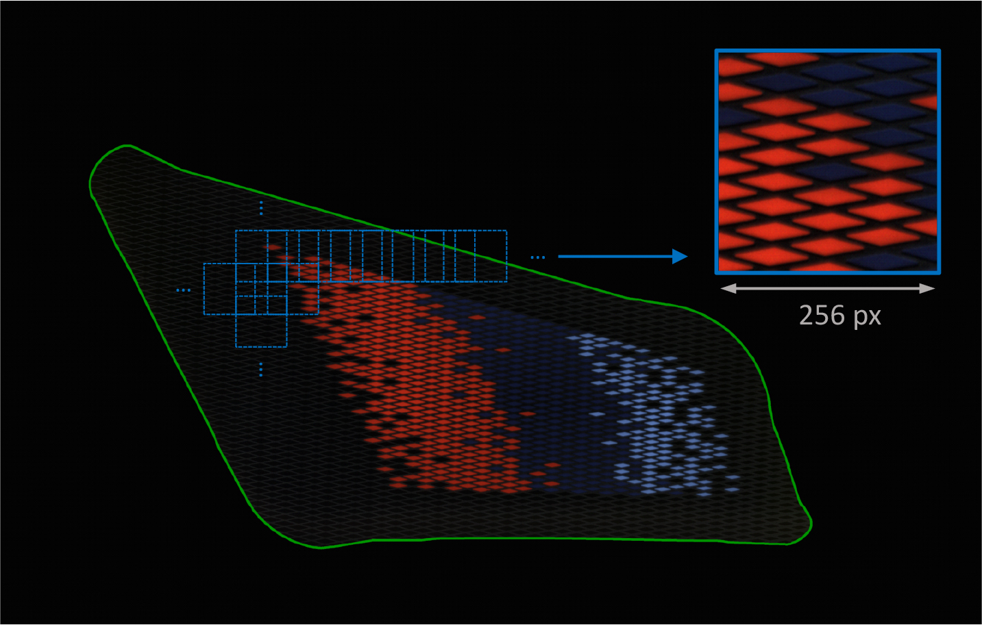
Illustration of the patch extraction process in the defined ROI. Overlapping patches (blue squares) are extracted within the entire ROI-area (green), ensuring a minimum covered sample area at the borders.
4.2Data processing
The images of the LSM-1 and LSM-2 measurement chambers consist of 16384
Figure 6.
Excerpts of masked sample images, acquired by means of the three measurement chambers: LSM-1, LSM-2 and ASM within a sequential run.
4.3Calibration and image acquisition
The calibration of the measurement modalities included optimizations of the rotary encoder settings, photo responsive non-uniformity corrections, fixed pattern noise corrections as well as white balancing. Depending on the modality, minimum exposure times of 100
5.Defect detection methods
The characteristics of the surface defects to be detected and the processing of large amounts of data within the production related cycle times pose a challenge for the selection of suitable defect detection methods. The evaluation of thousands of patches, most of which are fault-free, results in an imbalanced data distribution. In addition to a low false positive rate, defect detection methods are required that exhibit sufficient inference speed. In order to minimize the adaptation effort per product, defect detection methods with as little labeling effort as possible are preferred, while maintaining sufficient defect detection performance. The following section describes the defect detection methods utilized in each of the measurement chambers, as well as the data set preparation and method settings. As a baseline for benchmarking defect detection performance and inference speed, a state-of-the-art unsupervised anomaly detection method is introduced.
5.1Supervised oversampling method
A widely used approach in machine learning to compensate for imbalanced data distributions are resampling techniques such as random undersampling or oversampling [80, 81]. In the case of an imbalanced data distribution of majority and minority classes, the samples from the respective class are randomly eliminated (undersampling) or copied (oversampling) to create a revised balanced dataset. In the course of this work, a scalable patch-wise oversampling method is introduced that enables efficient use of scarce and imbalanced data available. The following steps are necessary in providing fault-free (majority class) and defective data (minority class):
1. Masking of the individual ROI’s of fault-free and defective samples and setting “out-of-ROI-values” to a integer value, e.g. zero.
2. Extraction of patches at random positions within the individual ROIs of the fault-free samples in the size of 512
3. Augmentation of the extracted patches using random affine transformations (rotation, shearing, etc.) and random color transformations (brightness, contrast, etc.).
4. Centre cropping of 1/2 of the original patch size (height, width) to avoid image borders, caused by augmentation.
5. The resulting fault-free and augmented patches of size 256
6. Extraction of defective patches of size 512
7. Training of a (pretrained) DCNN in a supervised manner, whereby the defective patches are injected with a probability of 50% into the stream of fault-free patches. This step utilizes the same augmentation settings as described in 3, including center cropping (256
Parameters such as the minimum ROI area covered per extracted patch and the maximum distance of random translations during augmentation, determined by defect type and patch size, must be carefully chosen. It is crucial to ensure that product surfaces are sufficiently represented and defects are covered after extraction and augmentation, to avoid e.g. generating defective patches that miss defective areas.
The samples used are pre-sorted by a domain expert prior to image acquisition, with separate samples for fault-free and defective data. This task eliminates any unwanted correlation between defective and fault-free patches in the subsequent data set generation. Thus, the labeling effort is limited only to the defective data at known regions, since the extraction of fault-free patches is integrated into an automated process (step 1 to 5). Furthermore no elaborate pixelwise labeling of ground truths as in in segmentation based approaches is required. By extracting patches at random positions, the original dataset can be exploited as much as possible (several 100 000 patches from a few acquired images with large FOVs). Moreover, it is theoretically possible to collect an endless stream of fault-free patches. Another advantage of patch-wise evaluation is that the patch context focuses on image features that are relevant for defect detection, while ignoring unimportant ones. As with other supervised methods that use oversampling techniques, attention must be given to possible overfitting. However, this method is easily scalable depending on data availability and thus can be fine-tuned as new defects emerge throughout the production process.
Above tasks can be seen as an applicable data-preparation as well as preprocessing workflow in industrial applications, reducing elaborate labeling only to known defective samples and sample regions.
5.2Synthetic defect method
Another method used in this publication is based on the synthesis of artificial defects [48]. This algorithm enables the synthetization of defects with a wide range of appearances, imitating a large proportion of real occurring defects. Basically, the synthetization algorithm consists of four steps:
1. Generation of a binary defect skeleton, that is based on a stochastic process resembling a random walk with momentum.
2. Generation of a random defect texture, based on the previously generated binary defect skeleton.
3. Modification of the fault-free image patch by means of the randomly generated defect texture.
4. Assessment of defect visibility and rejection of synthesized defects below the visibility threshold.
By utilizing different sets of hyperparameters of the random variables used in steps 1–3, it is possible to generate a variety of different defect morphologies (straight, jagged, curved, circular skeletons, etc.) and characteristics (contrast, intensity distribution). Depending on the appearance of the real defects to be imitated (elongated, punctual as in Fig. 2), the hyperparameters that determine the distribution of the random variables must be chosen selectively.
Due to the transition region of direct reflection as well as the frequent occurring ROI borders, above described method was adapted to generate visually apparent defects in both bright and dark contrasted areas, exclusively within the ROIs. Thus, defect synthetization categories and their underlying hyperparameters were adjusted based on real defects to produce bright and dark contrasted punctate and filamentous morphologies of different sizes and characteristics as depicted in Fig. 7. The preprocessing to generate the training and validation dataset follows almost the same procedure as steps 1–5 in Section 5.1. Additionally, following the central cropping in step 4, defects are generated in 50% of the fault-free patches. As a result, the generated training and validation datasets are balanced. With this method, it is therefore possible to perform balanced supervised training without the need for defective data. However, the generalization ability is only assessable using a test dataset containing real defects. Since the synthetization algorithm is based on grayscale, RGB images, if present, must either be converted or their channels processed independently.
Figure 7.
Synthetic generated defects on fault-free patches of LSM-1 (top row) and ASM (bottom row). Hyperparameters were chosen to mimic punctual and elongated “real” defects as shown in Fig. 2.
5.3Thresholding algorithm
LSM-2 enables the detection of pinholes, pattern misalignments or general inhomogeneities with low optical density. Due to the characteristics of the transmission measurement, defect features typically appear as white dots or areas of certain dimensions (Fig. 2, 2A/2C) within the image patch. To detect these features, a thresholding algorithm was developed, which is briefly described in the pseudo code of Algorithm 5.5.
The connected_components() function groups connected regions and assigns labels to the binarized image patches. These labels are then used to calculate the area of each defective region by counting the number of connected pixels per label. In order to utilize GPU-level parallelization the pseudo code shown in Algorithm 5.5 was implemented in a batchwise manner. With the help of this algorithm it is possible to tune parameters like RGB-thresholds and min. / max. defect areas, depending on the given quality requirements. As with other traditional image processing methods, no training data is demanded.
5.4Baseline method
The representation-based method by Roth et.al [32], namely PatchCore, is based on the extraction of mid-level features of fault-free patches using a pre-trained DCNN. During the training phase, subsamples of these locally aware patch features are stored in a memory bank. During inference, these features are compared to the extracted features of the image using a nearest neighbor search, resulting in anomaly scores. This method achieves SOTA anomaly detection performance on the MVTec dataset, resulting in an image-levelAUROC of up to 99.6%.
5.5Dataset and method settings
In order to evaluate methods described in section 5, image data were acquired by means of all three measurement chambers (LSM-1, LSM-2, ASM) of the inspection system demonstrator. Pre-sorted fault-free samples as well as defective samples of different defect classes were captured. The samples taken are in a state in which the printing process, including drying, has already been completed. Therefore, defects that occurred during printing are treated as fixed at this stage and no further significant changes are expected. However, the samples originate from different production batches and therefore have a desirable permitted design variability.
A training, validation and test dataset was created for each measurement modality. Each dataset consists of patches cropped from the respective ROIs of the acquired samples, resulting in an evaluation patch size of 256
0 -1
– Image Batch
– Threshold
– Maximum pixel sum above threshold
– Minimum and maximum feature areas
– Filter kernel size
– Image margin indices
– Predictions if patches are defective or fault-free
– Areas of connected components
patch in batch
patch[r] AND patch[g] AND patch[b]
dilated_patch
predictions
predictions, areas Thresholding Algorithm
5.5.1Supervised oversampling/synthetic defect training settings
For both methods, network training was performed using the stochastic gradient descent optimizer with parameters (learning rate as 5
5.5.2Thresholding algorithm settings
The thresholding algorithm (Algorithm 5.5) basically contains a set of seven values out of four parameters to be adjusted depending on the quality requirements e.g. defect sizes. The three threshold values of the RGB color channels, the min. and max. number of connected pixels above the previously set threshold, and a filter kernel size. The maximum pixel sum parameter is introduced for reasons of computational speed. Furthermore, it is possible to account for ignoring image margins in strided patch-wise extraction scenarios. Threshold values and other parameters were selected according to the best detection performance based on a predefined validation dataset as described in Section 5.5. Therefore, the optimal parameters were chosen as follows: Threshold RGB for all channels as 90 (uint8), min. and max. defect area as 1 and 3000, the maximum pixel sum as 15 000, the filter kernel size as 3. Patch margins with a size of 40 px were ignored during inference.
5.5.3Baseline settings: PatchCore
For reasons of adaptability, this paper investigates a self-implemented version according to [32]. As feature extractor, layers 2 and 3 of a ResNet50 resp. wide ResNet50 [85] pretrained on ImageNet were chosen with a kernel size of 3 and stride of 1 used for average pooling. IndexFlatL2 of the GPU-based Faiss library [86] was selected for feature embedding, while omitting coreset subsampling in order to exclude any defect detection performance loss. For all datasets, all available training patches were used for feature embedding, with the upper limit set to 500 and the number of nearest neighbors set to 3 resp. 5. Patch margins with a size of 40 px were ignored during feature embedding and evaluation of LSM-1 and LSM-2 to avoid common false positive detections in these areas. Furthermore, this is accompanied by an acceleration of inference speed. For LSM-1, an additional brightness adjustment was performed. As with the supervised methods above, the anomaly threshold for the binary classification task was chosen on the basis of the optimal F1-score. Prior to the experiments, the method was validated on the MVTec dataset and resulted in an average image level AUROC of 98.5% for image sizes of 256
All methods were implemented in Python (version
6.Method and inspection system evaluation
Experiments by means of the defect detection methods presented in Section 5 were conducted and evaluated regarding the patch-wise defect detection performance (Tables 1, 2) and the inference speed (Table 3). In addition, the overall inspection time of the implemented inspection system demonstrator was determined. As shown in Table 1, the defect detection performance is measured based on the entries in the confusion matrix, true negatives (TN), true positives (TP), false negatives (FN) and false positives (FP), and metrics obtained such as Matthews correlation coefficient (MCC) and false positive rate (FPR) as well as recall. Negatives correspond to fault-free patches, while positives represent defective ones. Commonly used metrics such as accuracy, F1-score or ROC-AUC are biased towards the majority class in the case of imbalanced data distributions. The MCC, with values ranging from
Table 1
Patch-wise defect detection performance metrics of leveraged methods; supervised oversampling method (Oversampling), synthetic defect method (Synthetic defects), threshold algorithm and the baseline method PatchCore. The test datasets are imbalanced to mimic typical inspection data distributions that overrepresent fault-free samples. The best performing method of each optical modality are highlighted in bold
| Modality | Method | #Real defects | TN | TP | FN | FP | MCC | Recall (%) | FPR (%) |
|---|---|---|---|---|---|---|---|---|---|
| LSM-1 | Oversampling | 42 | 1493 | 69 | 26 | 5 | 0.81 | 72.6 | 0.3 |
| 129 | 1495 | 77 | 18 | 3 | 0.88 | 81.1 | 0.2 | ||
| Synthetic defects | 0 | 1495 | 72 | 23 | 3 | 0.85 | 75.8 | 0.2 | |
| PatchCore | 0 | 1478 | 49 | 46 | 20 | 0.58 | 51.6 | 1.3 | |
| LSM-2 | Thresholding | 0 | 393 | 109 | 1 | 0 | 0.99 | 99.1 | 0.0 |
| PatchCore | 0 | 390 | 104 | 6 | 3 | 0.95 | 94.5 | 0.8 | |
| ASM | Synthetic defects | 0 | 2049 | 50 | 24 | 11 | 0.74 | 67.6 | 0.5 |
| PatchCore | 0 | 1954 | 29 | 45 | 106 | 0.26 | 39.2 | 5.1 |
6.1Patch-wise defect detection performance
The following section provides a detailed analysis of the method’s patch-wise defect detection performance, considering typical imbalanced inspection data distributions. The best performing method of each optical modality are highlighted in bold (Table 1). As in LSM-1, the supervised oversampling method achieved an MCC of 0.88 at an FPR of 0.2%, closely followed by synthetic defect training with an MCC of 0.85 and the same FPR. PatchCore resulted in a 6 times higher FPR and an MCC of 0.58. With the ASM setup, the best results were achieved through synthetic defect training with an MCC of 0.74 and an FPR of 0.5%. PatchCore performed even less well than in LSM-1, with an MCC of 0.26 and ten times higher FPR of 5.1%. In the absence of a sufficient number of defective samples, the supervised oversampling in ASM was skipped. Due to the clearly pronounced features in LSM-2, PatchCore performed robustly with an MCC of up to 0.95 and a comparatively low FPR of 0.8%. The thresholding algorithm presented in Algorithm 5.5 resulted in an MCC of 0.99 with only one overlooked defect.
Figure 8.
TP, FN and FP (columns) patch inference results of LSM-1, LSM-2 and ASM (rows) using PatchCore. Large area defects, such as the grid defect in 1A as well as the pattern misalignment in 2A produced clearly pronounced areas of anomaly. However, small and weakly contrasted point defects, such as the print defect and the pinhole (1B/2B), were overlooked. Feature variations in the vicinity of masked border regions (2C/3C) and transition regions of direct reflexion (3A) introduced many false positives.
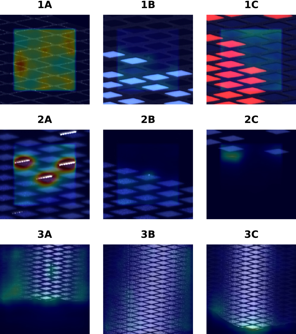
Figure 8 shows the inference results by means of the PatchCore method including anomaly overlay. Rows 1–3 follow the optical modalities LSM-1, LSM-2 and ASM. Columns A–C are arranged according to TP, FN and FP classification. The image margins ignored during inference are clearly visible in 1A–2C. Large area defects, such as the grid defect in 1A, produced clearly pronounced areas of anomaly, whereas point defects, such as the print defect in 1B, were overlooked. The high allowable variance of the structured pattern, as shown in 1C, led to a large amount of false positive patches. Large distinct defects, such as the pattern misalignment in 2A and high contrasted pinholes, produced large deviating feature vectors with respect to the learned feature embedding, leading to proper defect detection. However, small and low contrasted pinholes as illustrated in 2B were more likely to be missed. As with LSM-1, small feature variations in the vicinity of masked border regions also led to anomaly scores, resulting in false positives as in 2C. The ASM dataset poses a challenge regarding defect detection due to its high contrast variance in the transition region of direct reflection and its frequently appearing masked ROI regions. As shown in patches 3A and 3C, many false positives occurred at the border areas of the ROI as well as in before mentioned transition regions. Possible imperfect ROI segmentation also introduced additional feature variance, leading to false positives. Frequently, TP patches were classified as defective because of these detected regions, whereas large area defects such as squeegee strokes in 3B were partially or not detected at all.
Table 2
Patch-wise defect detection performance metrics comparing the methods supervised oversampling (Oversampling) and defect synthetization (Synthetic defects) by means of the defect groups Area and Points. The test datasets are imbalanced to mimic typical inspection data distributions that overrepresent fault-free samples. The best performing method of each defect group are highlighted in bold
| Modality | Defect group | Method | TN | TP | FN | FP | MCC | Recall (%) |
|---|---|---|---|---|---|---|---|---|
| LSM-1 | Area | Oversampling | 1498 | 49 | 0 | 3 | 0.97 | 100.0 |
| Synthetic defects | 1495 | 42 | 7 | 3 | 0.89 | 85.7 | ||
| ASM | 2049 | 14 | 19 | 11 | 0.48 | 42.4 | ||
| LSM-1 | Points | Oversampling | 1495 | 28 | 18 | 3 | 0.74 | 60.9 |
| Synthetic defects | 1495 | 30 | 16 | 3 | 0.76 | 65.2 | ||
| ASM | 2051 | 36 | 5 | 11 | 0.82 | 87.8 |
Table 2 illustrates the performance metrics obtained by means of the oversampling and synthetic defect methods in LSM-1 and ASM. For this purpose, the metrics previously shown in Table 1 were divided into their individual defect groups, point and area. In case of the supervised oversampling method in LSM-1, no area defect was overlooked, resulting in a recall of 100%. By utilizing synthetically generated defects as visualized in Fig. 7, a recall of 86% was obtained. Overall, area defects have not been synthesized and their morphology is completely different with respect to their optical modality in LSM-1 and ASM. This can be observed in Fig. 8, comparing the grid defect in 1A with the squeegee stroke defect in 3B. The grid defect contains punctate features, comparable to some synthesized point defects in LSM-1, thus potentially led to a robust recall of the above described 86%. The synthetic defect method performed slightly better than the supervised oversampling method in detecting point defects, resulting in a recall of 65%. In general, the detection of small sized defects in this modality is challenging, due to their weak appearance in surrounded structured patterns (Fig. 2 1A).
However, in the case of ASM, the detection of point defects was superior to LSM-1 with a recall of 88%. Although the morphology of the synthesized defects in ASM is completely different from that of area defects (as shown in Fig. 2, 3C), this defect group achieved a recall of 42%. This can be seen as the ability to learn the underlying distribution of the fault-free data using the influence of the vast amounts of augmented fault-free and synthetic defect patches.
Furthermore, the low FPR of 0.2–0.5% observed with these supervised learning procedures, with respect to the remaining high recall of certain defect groups, indicates strong generalization ability. Another indicator of its robustness is that possible imperfect ROI segmentations, such as those seen in ASM (e.g. holes within darkly contrasted ROI regions), which lead to false positives in PatchCore, are not noticeable during inference utilizing the synthetic defect method.
As shown in Table 1, the supervised oversampling method achieved an MCC of 0.81 and an FPR of 0.3% by leveraging a reduced set of 42 labeled defects. This gives an indication of the scalability of this method when compared to the metrics obtained using 129 labeled defects. As stated above 170–300 patches per ROI are evaluated, thus to avoid any false alarms FPR less than 0.59 resp. 0.33% are required to be applicable for inspection runs. Despite PatchCore, struggling with high FPR, introduced methods are capable of achieving even lower FPR.
6.2Inspection speed
In addition to the evaluation of defect detection performance, the inference speed of the applied defect detection methods was determined. As shown in Table 3, the inference times and their reciprocal, the throughput of patches per second, were measured in combination with their CUDA memory footprint. According to the image processing pipeline as described in Section 4.2, image batches with batch sizes of 128 were chosen for evaluation. However, in the case of PatchCore, the batch size was reduced to one. The use of large feature embeddings of 1.5 and 3.1 GiB resulted in a high computational GPU utilization of up to 91%, preventing any noticeable speed-up by means of larger batch sizes. The test image batches consisted of either dummy data sampled from a uniform distribution, or selected defective and fault-free patches yielding to torch tensors (float32) allocated on the GPU.
Table 3
Patch-wise inference speed measurements of utilized methods resp. their underlying architectures; supervised oversampling method and synthetic defect method (ResNet18), thresholding algorithm and the baseline method PatchCore
| Method | Data | Margin | Inference time | Throughput | Memory-Footprint |
|---|---|---|---|---|---|
| px | ms | patches/s | GiB | ||
| Thresholding | Dummy | 0 | 1.81 | 552 | 1.2 |
| 40 | 1.18 | 847 | |||
| Defective | 40 | 1.13 | 885 | ||
| Fault-free | 0 | 0.58 | 1724 | ||
| PatchCore | Defective | 0 | 118.89 | 8 | 6.0 |
| Defective | 40 | 32.95 | 30 | 4.5 | |
| ResNet18 | Dummy | 0 | 0.18 | 5556 | 2.3 |
The performance measures shown in Table 3 were determined using the arithmetic mean of 5 cycles with 100 repetitions, including preprocessing of the respective methods. Prior to each measurement cycles, a GPU warm-up of 10 repetitions was performed. To account for asynchronous CUDA data processing, inference times were measured using PyTorch’s synchronized CUDA events [88]. The GPU memory footprint of each method was determined using torch.cuda.mem_get_info(), deducting PyTorch’s CUDA context of approximately 1.3 GiB.
As expected, the ResNet18 architecture, used by means of the supervised oversampling and the synthetic defect method, achieved the lowest inference time of 0.18 ms, resulting in a throughput of 5556 patches/s. Inference times larger than 1000 patches/s have already been reported for ResNet architectures in [89]. The dependence of the threshold algorithm on the input data is clearly visible in Table 3. The highest inference time was measured with 1.81 ms in the case of the dummy data and 0.58 ms for fault-free data, missing defective pixels and thus skipping the computation of defective areas. These values represent the estimated upper and lower bounds. Thus, in an industrial setting with a majority of fault-free patches per batch, throughputs of up to 1724 patches/s can be achieved. Due to the exhaustive nearest neighbor search in large feature embeddings, PatchCore led to by far the highest inference times of 32.95 and 118.89 ms. This means that both the thresholding algorithm and the methods that utilize the ResNet18 are approx. 57–183 times faster compared to the PatchCore configuration, that ignores image margins. Although, ignoring image margins for feature embedding and subsequent feature comparison led to a approx. 3.6 times reduction in inference time. For comparison, a thorough evaluation of SOTA anomaly detection methods inference speeds, including PatchCore, can be explored on p. 21 in [35]. The proposed method, namely EfficientAD, achieved the highest throughput of up to 614 patches/s, including CPU to GPU transfers. Thus, in inspection settings described above, embedding-based methods like PatchCore would lead to bottleneck the overall inspection process, not achieving required cycle times. In terms of memory footprint, the thresholding algorithm exhibits the smallest value with 1.2 GiB, followed by ResNet18 with 2.3 Gib and PatchCore with up to 6.0 GiB.
6.3Inspection system demonstrator performance
The inference times determined above do not include all data processing steps during defect inspection as described in Section 4.2, such as registration, ROI segmentation or patch extraction, etc. To account for these computationally intensive tasks and to estimate the overall inspection time of the implemented inspection system demonstrator, separate runs of the samples through all measurement chambers were performed. The best performing methods regarding defect detection performance (bold in Table 1) were therefore chosen for each modality. The time measurements started at the onset of image acquisition in LSM-1 and ended after finishing the post-processing of all modalities to ensure the availability of patch-wise inference results. A total of 10 inspection runs with various samples resulted in an average inspection time of 20.25
In terms of defect detection performance, it was qualitatively observed that the used defect detection methods are capable of detecting the wide range of different defect classes with high sensitivity at low false positive rates, confirming the metrics in Table 1. In the case of LSM-1, small defects that differ only slightly from their surroundings are more likely to be overlooked than area defects that are pronounced over the entire ROI. Despite the observation of missed defects (mostly area defects) in the test dataset of ASM resulting in a relatively low MCC of 0.74 compared to other modalities, this was not the case when performing inspection. Due to the high frame rates in ASM, the possibility of a defect occurring in more than one patch as well as in different illumination regions is increased and thus counteracts the determined dataset-specific recall. However, a thorough quantitative evaluation of the system’s defect detection performance, considering the quality standards of the project partner, should be carried out in the future.
7.Conclusions and outlook
This work presents a novel automatic visual inspection system for decorated foil plates, applicable for full-surface defect detection. Developed optical modalities embedded in a sequential inspection procedure, enable defect visualization of production related defect classes with sufficient contrast. Thereby, applicability and adaptability to various product sizes with FOV’s of up to 1200 mm as well as different product designs is ensured. Introduced patch-wise defect detection methods namely, supervised oversampling-, synthetic defect method as well as the thresholding algorithm are applicable for full-surface defect detection of small defects (few px in extension) in relation to large sized samples of up to 106 mm2. Therefore, defect detection performance and inference speeds considering inspection related requirements such as e.g. FPR and cycle times were determined. The synthetic defect method as well as the thresholding algorithm do not rely on any labeled defective training data. By means of these methods it was possible to achieve MCC’s of up to 0.85 resp. 0.99, thus outperforming SOTA unsupervised anomaly detection method PatchCore. The obtained metrics of the synthetic defect method underline their applicability on structured patterns, although the determination of suitable hyperparameters is time-consuming. Its automatization would be beneficial for increasing further usability.
In terms of defect inspection, area defects that are pronounced over large sample areas are statistically more likely to be detected by patch-wise inference than the less sampled point defects. Additionally, area defects are more apparent than weakly pronounced point defects in terms of defect visualization. Furthermore, area defects, such as pattern misalignments, generate numerous defective patches per sample that can be used for subsequent training. Thus, point defects are more relevant to defect synthesis as they are easier to overlook and more sparse.
Furthermore, an industry-applicable data preprocessing workflow has been introduced, minimizing the labeling effort in supervised settings. This workflow leverages the automatic extraction of patches from preselected fault-free samples, eliminating the need for exhaustive screening of thousands of patches. Overlooked defects, such as potential process contamination, had no significant impact on the training process. This is likely due to the extraction of a large number of patches (100 000) and the clean sample preparation by domain experts. Thus, manual labeling is limited to the extraction of defective patches at known positions on separate defective samples. This scalable balanced learning procedure is able to achieve the demanded FPR as well as recall, due to the possible utilization of available fault-free resp. defective samples during production. The proposed workflow is not limited to screen-printed products with flat surfaces. Tests on 3D-shaped products using additional viewpoints indicated its applicability to various industrial manufacturing processes (e.g. injection molding, forging, additive manufacturing), minimizing the overall labeling effort.
Defect detection of small and weakly pronounced defects in its underlying structured patterns remain challenging as in case of point defects in LSM-1. Optimization in recall could be obtained by separately training of area and point defect groups, assuming sufficient defective data is available for each class. Additionally, subsequent classification of individual defect classes would be possible enabling logging of defects statistics. Exploiting fault-free data of all modalities and performing a self-supervised pretext task (e.g. with synthetic defects) would generate a robust feature extractor, applicable for subsequent fine-tuning with collected defective samples on same or similar patterns. Furthermore, including available defective data samples during synthetic defect training as presented in [90] would be another viable strategy in improving detection performance.
Regarding the thresholding algorithm, attention has to be given to product designs with low optical density, introducing possible false alarms. One strategy could be appropriate masking ignoring these specific regions. In case of defect visualization in ASM, one has to keep in mind that orientation dependent defect classes such as e.g. weak appearing squeegee strokes might be overlooked. Therefore, proper sample alignment must be ensured prior to inspection. In addition, attention must be given to the presence of contamination such as dust in the inspection environment to avoid potential false alarms. The possible in-line integration of the inspection system into a closed manufacturing cycle is part of further research work.
It can be highlighted that the evaluation of methods to be capable for industry applications is highly dependent on the experimental design. This includes proper dataset generation mimicking the imbalanced inspection scenario as well as choosing suitable performance metrics. The choice of demanded recall and precision is dependent on the quality requirements of the application as well as on the method itself, e.g. patch-wise processing. Enabling demanded defect detection performance among required inspection speeds is challenging, thus further research has to be conducted regarding industry applicable defect detection methods. Due to fast emerging unsupervised anomaly detection methods as listed in [33, 34, 35, 41, 44], it is planned to investigate their capability of defect detection on these challenging structured patterns in future research.
Acknowledgments
The research work was performed within the COMET-project “Deep on-line learning for highly adaptable polymer surface inspection systems” (project-no.: 879785) at the Polymer Competence Center Leoben GmbH (PCCL, Austria) within the framework of the COMET-program of the Federal Ministry for Climate Action, Environment, Energy, Mobility, Innovation and Technology and the Federal Ministry for Digital and Economic Affairs and with contributions by Burg Design GmbH. The PCCL is funded by the Austrian Government and the State Governments of Styria, Lower Austria and Upper Austria.
References
[1] | See JE, Drury CG, Speed A, Williams A, Khalandi N. The Role of Visual Inspection in the 21st Century. Proceedings of the Human Factors and Ergonomics Society Annual Meeting. (2017) ; 61: (1): 262-6. Available from: doi: 10.1177/. |
[2] | Peres RS, Jia X, Lee J, Sun K, Colombo AW, Barata J. Industrial Artificial Intelligence in Industry 4.0 – Systematic Review, Challenges and Outlook. IEEE Access. (2020) ; 8: : 220121-39. |
[3] | Aminabadi SS, Tabatabai P, Steiner A, Gruber DP, Friesenbichler W, Habersohn C, et al. Industry 4.0 In-Line AI Quality Control of Plastic Injection Molded Parts. Polymers. (2022) ; 14: (17). |
[4] | Javaid M, Haleem A, Singh RP, Rab S, Suman R. Exploring impact and features of machine vision for progressive industry 4.0 culture. Sensors International. (2022) ; 3: : 100132. |
[5] | Ruiz L, González J, Cavas F. Improving the competitiveness of aircraft manufacturing automated processes by a deep neural network. Integrated Computer-Aided Engineering. (2023) 05; 30: : 1-12. |
[6] | Chin RT, Harlow CA. Automated Visual Inspection: A Survey. IEEE Transactions on Pattern Analysis and Machine Intelligence. (1982) ; PAMI-4: (6): 557-73. |
[7] | Ren Z, Fang F, Yan N, Wu Y. State of the Art in Defect Detection Based on Machine Vision. International Journal of Precision Engineering and Manufacturing-Green Technology. (2022) ; 9: (2): 661-91. |
[8] | Silva RL, Rudek M, Szejka AL, Junior OC. Machine Vision Systems for Industrial Quality Control Inspections. In: Chiabert P, Bouras A, Noël F, Ríos J, editors. Product Lifecycle Management to Support Industry 4.0 Cham: Springer International Publishing; (2018) . pp. 631-41. |
[9] | Ebayyeh AARMA, Mousavi A. A Review and Analysis of Automatic Optical Inspection and Quality Monitoring Methods in Electronics Industry. IEEE Access. (2020) ; 8: : 183192-271. |
[10] | Huang SH, Pan YC. Automated visual inspection in the semiconductor industry: A survey. Computers in Industry. (2015) ; 66: : 1-10. Available from: https://www.sciencedirect.com/science/article/pii/s0166361514001845 https://www.sciencedirect.com/science/article/pii/s0166361514001845. |
[11] | Kumar A. Computer-Vision-Based Fabric Defect Detection: A Survey. IEEE Transactions on Industrial Electronics. (2008) ; 55: (1): 348-63. |
[12] | Hanbay K, Talu MF, Özgüven ÖF. Fabric defect detection systems and methods – A systematic literature review. Optik. (2016) ; 127: (24: 11960-73. Available from: https://www.sciencedirect.com/science/article/pii/s0030402616311366 https://www.sciencedirect.com/science/article/pii/s0030402616311366. |
[13] | Kuo CFJ, Wang WR, Barman J. Automated Optical Inspection for Defect Identification and Classification in Actual Woven Fabric Production Lines. Sensors. (2022) ; 22: (19): 7246. Available from: https://www.mdpi.com/1424-8220/22/19/7246. |
[14] | Vans M, Schein S, Staelin C, Kisilev P, Simske S, Dagan R, et al. Automatic visual inspection and defect detection on variable data prints. Journal of Electronic Imaging. (2011) ; 20: (1): 013010-0. |
[15] | Zhang E, Chen Y, Gao M, Duan J, Jing C. Automatic Defect Detection for Web Offset Printing Based on Machine Vision. Applied Sciences. (2019) ; 9: (17): 3598. Available from: https://www.mdpi.com/2076-3417/9/17/3598 https://www.mdpi.com/2076-3417/9/17/3598. |
[16] | Sun N, Cao B. Real-Time Image Defect Detection System of Cloth Digital Printing Machine. Computational Intelligence and Neuroscience. (2022) ; 2022: : 5625945. Available from: https://www.hindawi.com/journals/cin/2022/5625945/https://www.hindawi.com/journals/cin/2022/5625945/. |
[17] | Hachem CE, Perrot G, Painvin L, Couturier R. Automation of Quality Control in the Automotive Industry Using Deep Learning Algorithms. In: 2021 International Conference on Computer, Control and Robotics (ICCCR); (2021) . pp. 123-7. |
[18] | Zhou Q, Chen R, Huang B, Liu C, Yu J, Yu X. An Automatic Surface Defect Inspection System for Automobiles Using Machine Vision Methods. Sensors. (2019) ; 19: (3): 644. Available from: https://www.mdpi.com/1424-8220/19/3/644. |
[19] | Gruber DP, Macher J, Haba D, Berger GR, Pacher G, Friesenbichler W. Measurement of the visual perceptibility of sink marks on injection molding parts by a new fast processing model. Polymer Testing. (2014) ; 33: : 7-12. |
[20] | Gospodnetić P, Hirschenberger F. Detection and Visibility Estimation of Surface Defects Under Various Illumination Angles Using Bidirectional Distribution Function and Local Binary Pattern. In: Lončarić S, Cupec R, editors. Proceedings of the Croatian Compter Vision Workshop, Year 4. Center of Excellence for Computer Vision. Osijek: University of Zagreb; (2016) . pp. 9-14. Available from: doi: 10.20532/ccvw.2016.0002. |
[21] | Lin HI, Wibowo FS. Image Data Assessment Approach for Deep Learning-Based Metal Surface Defect-Detection Systems. IEEE Access. (2021) ; 9: : 47621-38. |
[22] | Ultraviolet (UV) Image Sensor | Products & Solutions | Sony Semiconductor Solutions Group [homepage on the Internet]; cited 2024-05-28. Available from: https://www.sony-semicon.com/en/products/is/industry/uv.html https://www.sony-semicon.com/en/products/is/industry/uv.html. |
[23] | Hashagen J. Seeing Beyond the Visible. Optik & Photonik. (2015) ; 10: (3): 34-7. |
[24] | Amigo JM, Grassi S. Configuration of hyperspectral and multispectral imaging systems. In: Hyperspectral Imaging. vol. 32 of Data Handling in Science and Technology. Elsevier; (2019) . pp. 17-34. |
[25] | Feng CH, Makino Y, Oshita S, García Martín JF. Hyperspectral imaging and multispectral imaging as the novel techniques for detecting defects in raw and processed meat products: Current state-of-the-art research advances. Food Control. (2018) ; 84: : 165-76. |
[26] | Calvini R, Ulrici A, Amigo JM. Growing applications of hyperspectral and multispectral imaging. In: Hyperspectral Imaging. vol. 32 of Data Handling in Science and Technology. Elsevier; (2019) . pp. 605-29. |
[27] | Serranti S, Bonifazi G. Hyperspectral imaging and its applications. In: Berghmans F, Mignani AG, editors. Optical Sensing and Detection IV. SPIE Proceedings. SPIE; (2016) ; p. 98990P. |
[28] | Prunella M, Scardigno RM, Buongiorno D, Brunetti A, Longo N, Carli R, et al. Deep Learning for Automatic Vision-Based Recognition of Industrial Surface Defects: A Survey. IEEE Access. (2023) ; 11: : 43370-423. |
[29] | Qi S, Yang J, Zhong Z. A Review on Industrial Surface Defect Detection Based on Deep Learning Technology. In: 2020 The 3rd International Conference on Machine Learning and Machine Intelligence. New York, NY, USA: ACM; (2020) . pp. 24-30. |
[30] | Jin Q, Chen L. A survey of surface defect detection of industrial products based on a small number of labeled data. arXiv preprint arXiv:220305733. (2022) . Available from: doi: 10.48550/arXiv.2203.05733. |
[31] | Bergmann P, Batzner K, Fauser M, Sattlegger D, Steger C. The MVTec Anomaly Detection Dataset: A Comprehensive Real-World Dataset for Unsupervised Anomaly Detection. International Journal of Computer Vision. (2021) ; 129: (4): 1038-59. |
[32] | Roth K, Pemula L, Zepeda J, Scholkopf B, Brox T, Gehler P. Towards Total Recall in Industrial Anomaly Detection. In: 2022 IEEE/CVF Conference on Computer Vision and Pattern Recognition (CVPR). IEEE Computer Society; 6/18/2022–6/24/2022. pp. 14298-308. |
[33] | Xie G, Wang J, Liu J, Zheng F, Jin Y. Pushing the Limits of Fewshot Anomaly Detection in Industry Vision: Graphcore. arXiv e-prints. 2023. Available from: https://arxiv.org/pdf/2301.12082.pdfhttps://arxiv.org/pdf/2301.12082.pdf. |
[34] | Li H, Hu J, Li B, Chen H, Zheng Y, Shen C. Target before Shooting: Accurate Anomaly Detection and Localization under One Millisecond via Cascade Patch Retrieval. arXiv e-prints. 2023. Available from: https://arxiv.org/pdf/2308.06748v1.pdf. |
[35] | Batzner K, Heckler L, König R. EfficientAD: Accurate Visual Anomaly Detection at Millisecond-Level Latencies. arXiv e-prints. 2023. Available from: https://arxiv.org/pdf/2303.14535.pdfhttps://arxiv.org/pdf/2303.14535.pdf. |
[36] | Bergmann P, Löwe S, Fauser M, Sattlegger D, Steger C. Improving Unsupervised Defect Segmentation by Applying Structural Similarity to Autoencoders. (2019) ; 372-80. Available from: https://arxiv.org/pdf/1807.02011v3. |
[37] | Zavrtanik V, Kristan M, Skočaj D. DRAEM – A Discriminatively Trained Reconstruction Embedding for Surface Anomaly Detection. In: Proceedings of the IEEE/CVF International Conference on Computer Vision (ICCV); (2021) ; pp. 8330-9. |
[38] | Schlegl T, Seeböck P, Waldstein SM, Schmidt-Erfurth U, Langs G. Unsupervised anomaly detection with generative adversarial networks to guide marker discovery. In: International conference on information processing in medical imaging. Springer; (2017) ; pp. 146-57. |
[39] | Zhang L, Dai Y, Fan F, He C. Anomaly Detection of GAN Industrial Image Based on Attention Feature Fusion. Sensors (Basel, Switzerland). (2022) ; 23: (1). |
[40] | Zhang H, Wang Z, Wu Z, Jiang YG. Diffusionad: Denoising diffusion for anomaly detection. arXiv preprint arXiv: 230308730. 2023. Available from: doi: 10.48550/arXiv.2303.08730. |
[41] | Mousakhan A, Brox T, Tayyub J. Anomaly Detection with Conditioned Denoising Diffusion Models. arXiv e-prints. 2023. Available from: https://arxiv.org/pdf/2305.15956.pdf. |
[42] | Tebbe J, Tayyub J. D3AD: Dynamic Denoising Diffusion Probabilistic Model for Anomaly Detection. arXiv preprint arXiv:240104463. 2024. Available from: doi: 10.48550/arXiv.2401.04463. |
[43] | Yu J, Zheng Y, Wang X, Li W, Wu Y, Zhao R, et al. FastFlow: Unsupervised Anomaly Detection and Localization via 2D Normalizing Flows. arXiv e-prints. 2021. Available from: https://arxiv.org/pdf/2111.07677.pdf. |
[44] | Zhou Y, Xu X, Song J, Shen F, Shen HT. MSFlow: Multi-Scale Flow-based Framework for Unsupervised Anomaly Detection. arXiv e-prints. 2023. Available from: https://arxiv.org/pdf/2308.15300v1.pdfhttps://arxiv.org/pdf/2308.15300v1.pdf. |
[45] | Deng J, Dong W, Socher R, Li LJ, Li K, Fei-Fei L. Imagenet: A large-scale hierarchical image database. In: 2009 IEEE conference on computer vision and pattern recognition. IEEE; (2009) . pp. 248-55. |
[46] | Goodfellow I, Pouget-Abadie J, Mirza M, Xu B, Warde-Farley D, Ozair S, et al. Generative adversarial nets. Advances in Neural Information Processing Systems. (2014) ; 27: . |
[47] | Li CL, Sohn K, Yoon J, Pfister T. Cutpaste: Self-supervised learning for anomaly detection and localization. In: Proceedings of the IEEE/CVF conference on computer vision and pattern recognition; (2021) ; pp. 9664-74. |
[48] | Haselmann M, Gruber D. Supervised Machine Learning Based Surface Inspection by Synthetizing Artificial Defects. In: International Conference on Machine Learning and Applications Cancún Mt, editor. ICMLA 2017: proceedings 16th IEEE International Conference on Machine Learning and Applications: 18–21 December 2017, Cancun, Mexico. IEEE; (2017) . pp. 390-5. |
[49] | Niu S, Li B, Wang X, Lin H. Defect Image Sample Generation With GAN for Improving Defect Recognition. IEEE Transactions on Automation Science and Engineering. (2020) ; 1-12. |
[50] | He X, Luo Z, Li Q, Chen H, Li F. DG-GAN: A High Quality Defect Image Generation Method for Defect Detection. Sensors (Basel, Switzerland). (2023) ; 23: (13). |
[51] | Zhong X, Zhu J, Liu W, Hu C, Deng Y, Wu Z. An Overview of Image Generation of Industrial Surface Defects. Sensors. (2023) ; 23: (19): 8160. |
[52] | Duan Y, Hong Y, Niu L, Zhang L. Few-shot defect image generation via defect-aware feature manipulation. In: Proceedings of the AAAI Conference on Artificial Intelligence. vol. 37: ; (2023) . pp. 571-8. |
[53] | Hu T, Zhang J, Yi R, Du Y, Chen X, Liu L, et al. Anomalydiffusion: Few-shot anomaly image generation with diffusion model. In: Proceedings of the AAAI Conference on Artificial Intelligence. vol. 38: ; (2024) . pp. 8526-34. |
[54] | Tai Y, Yang K, Peng T, Huang Z, Zhang Z. Defect Image Sample Generation With Diffusion Prior for Steel Surface Defect Recognition. arXiv preprint arXiv:240501872. (2024) . Available from: doi: 10.48550/arXiv.2405.01872. |
[55] | Capogrosso L, Girella F, Taioli F, Chiara M, Aqeel M, Fummi F, et al. Diffusion-Based Image Generation for In-Distribution Data Augmentation in Surface Defect Detection. In: Proceedings of the 19th International Joint Conference on Computer Vision, Imaging and Computer Graphics Theory and Applications-(Volume 2). SciTePress; (2024) . pp. 409-16. |
[56] | Zhao Z, Li B, Liu T, Zhang S, Lu J, Geng L, et al. Visual inspection system for battery screen print using joint method with multi-level block matching and K nearest neighbor algorithm. Optik. (2022) ; 250: : 168332. Available from: https://www.sciencedirect.com/science/article/pii/S0030402621018453 https://www.sciencedirect.com/science/article/pii/S0030402621018453. |
[57] | Jiang J, Cao P, Lu Z, Lou W, Yang Y. Surface Defect Detection for Mobile Phone Back Glass Based on Symmetric Convolutional Neural Network Deep Learning. Applied Sciences. (2020) ; 10: (10): 3621. |
[58] | Yuan ZC, Zhang ZT, Su H, Zhang L, Shen F, Zhang F. Vision-Based Defect Detection for Mobile Phone Cover Glass using Deep Neural Networks. International Journal of Precision Engineering and Manufacturing. (2018) ; 19: (6): 801-10. |
[59] | Zhou Z, Rahman Siddiquee MM, Tajbakhsh N, Liang J. UNet++: A Nested U-Net Architecture for Medical Image Segmentation. In: International Conference on Machine Learning and Applications Cancún Mt, editor. ICMLA 2017: proceedings 16th IEEE International Conference on Machine Learning and Applications: 18–21 December 2017, Cancun, Mexico. IEEE; (2017) . pp. 3-11. Available from: https://link.springer.com/chapter/10.1007/978-3-030-00889-5_1 https://link.springer.com/chapter/10.1007/978-3-030-00889-5_1. |
[60] | Yoon B, Lee H, Jeong J. Improved U-Net++ with Patch Split for Micro-Defect Inspection in Silk Screen Printing. Applied Sciences. (2022) ; 12: (9): 4679. |
[61] | Gafurov AN, Phung TH, Ryu BH, Kim I, Lee TM. AI-Aided Printed Line Smearing Analysis of the Roll-to-Roll Screen Printing Process for Printed Electronics. International Journal of Precision Engineering and Manufacturing-Green Technology. (2023) ; 10: (2): 339-52. |
[62] | Deltamax [homepage on the Internet]; cited 2024-02-07. Available from: https://deltamax.eu/en/products/glassinspector/. |
[63] | Elunic [homepage on the Internet]; cited 2024-02-07. Available from: https://www.elunic.com/de/aisee/qualitaetssicherung-presswerk-ki/ https://www.elunic.com/de/aisee/qualitaetssicherung-presswerk-ki/. |
[64] | Lake Image [homepage on the Internet]; cited 2024-02-07. Available from: https://lakeimage.com/products/discovery-roll-inspector/ https://lakeimage.com/products/discovery-roll-inspector/. |
[65] | Nireco Corporation [homepage on the Internet]; cited 2024-02-07. Available from: https://nireco.com/en/product/surface-inspection/mujiken-plus.html https://nireco.com/en/product/surface-inspection/mujiken-plus.html. |
[66] | Solomon [homepage on the Internet]. cited 2024-02-07. Available from: https://www.solomon-3d.com/solomon-vision. |
[67] | Stoba [homepage on the Internet]; cited 2024-02-07. Available from: https://www.stoba.one/en/customized-machinery/technologies/visual-inspection https://www.stoba.one/en/customized-machinery/technologies/visual-inspection. |
[68] | Dr. Schenk GmbH [homepage on the Internet]; cited 2024-02-07. Available from: https://www.drschenk.com/products.html. |
[69] | ColorBrain [homepage on the Internet]; cited 2024-02-07. Available from: https://www.baumerinspection.com/us/en/baumer-inspection-navigation/products/colourbrain-decoinspector/a/decoinspector https://www.baumerinspection.com/us/en/baumer-inspection-navigation/products/colourbrain-decoinspector/a/decoinspector. |
[70] | In-Core Systemes [homepage on the Internet]; cited 2024-02-07. Available from: https://www.incore-systemes.com/composites-materials/ https://www.incore-systemes.com/composites-materials/. |
[71] | Omso [homepage on the Internet]; cited 2024-02-07. Available from: https://www.omso.it/en/p/ecolin. |
[72] | Cugher [homepage on the Internet]. cited 2024-02-07. Available from: https://www.cugher.com/increased-quality-control-and-production-monitoring-for-industry-4-0 https://www.cugher.com/increased-quality-control-and-production-monitoring-for-industry-4-0. |
[73] | Keko Equipment [homepage on the Internet]; cited 2024-02-07. Available from: https://www.keko-equipment.com/Inspection.php https://www.keko-equipment.com/Inspection.php. |
[74] | Sakurai Graphic Systems Corporation [homepage on the Internet]; cited 2024-02-07. Available from: https://www.sakurai-gs.co.jp/en/products/process/si.html https://www.sakurai-gs.co.jp/en/products/process/si.html. |
[75] | Krassnig PJ, Haselmann M, Gruber DP. Inspection Approach for Automated In-line Defect Detection on Decorated Foil Plates. Advances in Signal Processing and Artificial Intelligence: Proceedings of the 4th International Conference on Advances in Signal Processing and Artificial Intelligence 19–21 October 2022 Corfu, Greece. (2022) : 84-5. |
[76] | Biegeleisen JI. Complete Book of Silk Screen Printing Production. Dover Publications; (2012) ; Available from: https://books.google.at/books?id=o8sKJSHeU-MC https://books.google.at/books?id=o8sKJSHeU-MC. |
[77] | Sauer M, Meilchen S, Kalleder A, Mennig M, Schmidt H. Screen Printing. In: Aegerter MA, editor. Sol gel technologies for glass producers and users. New York, NY: Springer Science |
[78] | Handbook for screen printers. Thal, Switzerland: Sefar; (2006) . |
[79] | ISO 12233:2000(en) [homepage on the Internet]; cited 2024-02-07. Available from: https://www.iso.org/obp/ui. |
[80] | Haixiang G, Yijing L, Shang J, Mingyun G, Yuanyue H, Bing G. Learning from class-imbalanced data: Review of methods and applications. Expert Systems with Applications. (2017) ; 73: : 220-39. Available from: https://www.sciencedirect.com/science/article/pii/S0957417416307175 https://www.sciencedirect.com/science/article/pii/S0957417416307175. |
[81] | He H, Garcia EA. Learning from Imbalanced Data. IEEE Transactions on Knowledge and Data Engineering. (2009) ; 21: (9): 1263-84. |
[82] | Hambardzumyan S, Tuli A, Ghukasyan L, Rahman F, Topchyan H, Isayan D, et al. Deep Lake: a Lakehouse for Deep Learning. arXiv e-prints. 2022arXiv:2209.10785. |
[83] | He K, Zhang X, Ren S, Sun J. Deep Residual Learning for Image Recognition. In: Proceedings of the IEEE Conference on Computer Vision and Pattern Recognition (CVPR); (2016) . |
[84] | Loshchilov I, Hutter F. SGDR: Stochastic Gradient Descent with Warm Restarts. arXiv e-prints. 2016. Available from: https://arxiv.org/pdf/1608.03983.pdf https://arxiv.org/pdf/1608.03983.pdf. |
[85] | Zagoruyko S, Komodakis N. Wide Residual Networks. arXiv e-prints. 2016. Available from: https://arxiv.org/pdf/1605.07146.pdf https://arxiv.org/pdf/1605.07146.pdf. |
[86] | Johnson J, Douze M, Jegou H. Billion-Scale Similarity Search with GPUs. IEEE Transactions on Big Data. (2021) ; 7: (3): 535-47. |
[87] | Chicco D, Jurman G. The Matthews correlation coefficient (MCC) should replace the ROC AUC as the standard metric for assessing binary classification. BioData Mining. (2023) ; 16: (1): 4. Available from: https://biodatamining.biomedcentral.com/articles/10.1186/s13040-023-00322-4 https://biodatamining.biomedcentral.com/articles/10.1186/s13040-023-00322-4. |
[88] | Event – PyTorch 2.1. documentation [homepage on the Internet]; cited 2024-02-07. Available from: https://pytorch.org/docs/stable/generated/torch.cuda.Event.html https://pytorch.org/docs/stable/generated/torch.cuda.Event.html. |
[89] | Bianco S, Cadene R, Celona L, Napoletano P. Benchmark Analysis of Representative Deep Neural Network Architectures. IEEE Access. (2018) ; 6: : 64270-7. |
[90] | Haselmann M, Krassnig PJ, Gruber DP. Visual inspection of patterned surfaces with supervised deep learning using both real and synthetic defects. Advances in Signal Processing and Artificial Intelligence: Proceedings of the 4th International Conference on Advances in Signal Processing and Artificial Intelligence 19–21 October 2022 Corfu, Greece. (2022) : 138-9. |


