
A General Framework for Providing Interval Representations of Pareto Optimal Outcomes for Large-Scale Bi- and Tri-Criteria MIP Problems
Abstract
The Multi-Objective Mixed-Integer Programming (MOMIP) problem is one of the most challenging. To derive its Pareto optimal solutions one can use the well-known Chebyshev scalarization and Mixed-Integer Programming (MIP) solvers. However, for a large-scale instance of the MOMIP problem, its scalarization may not be solved to optimality, even by state-of-the-art optimization packages, within the time limit imposed on optimization. If a MIP solver cannot derive the optimal solution within the assumed time limit, it provides the optimality gap, which gauges the quality of the approximate solution. However, for the MOMIP case, no information is provided on the lower and upper bounds of the components of the Pareto optimal outcome. For the MOMIP problem with two and three objective functions, an algorithm is proposed to provide the so-called interval representation of the Pareto optimal outcome designated by the weighting vector when there is a time limit on solving the Chebyshev scalarization. Such interval representations can be used to navigate on the Pareto front. The results of several numerical experiments on selected large-scale instances of the multi-objective multidimensional 0–1 knapsack problem illustrate the proposed approach. The limitations and possible enhancements of the proposed method are also discussed.
1Introduction
The derivation of optimal solutions to large-scale instances of the Mixed-Integer Programming (MIP) problem can be impossible within a reasonable time limit even for contemporary commercial MIP solvers, e.g. GUROBI (Gurobi, 2023), CPLEX (IBM, 2023). In this case, a MIP solver provides the optimality gap (MIP gap) that gauges the quality of the approximate solution, i.e. the last feasible solution (incumbent). This optimality gap is calculated based on the incumbent and the so-called MIP best bound.
In the case of the Multi-Objective MIP (MOMIP) problem, scalarization techniques and MIP solvers can be used to derive Pareto optimal solutions (see, e.g. Miettinen, 1999; Ehrgott, 2005). Examples of applying MIP packages to solve multi-criteria decision problems are shown in, e.g. Ahmadi et al. (2012), Delorme et al. (2014), Eiselt and Marianov (2014), Oke and Siddiqui (2015), Samanlioglu (2013). As a scalarization technique, one can use the Chebyshev scalarization that guarantees the derivation of each (properly) Pareto optimal solution (see, e.g. Kaliszewski, 2006). Other advantages of using this scalarization in the context of decision-making and expressing the decision maker’s preferences are discussed in, e.g. Miroforidis (2021).
In the current work, we say that an instance of the MOMIP problem is large-scale if its Chebyshev scalarization cannot be solved to optimality by a MIP solver within an assumed time limit that is reasonable in the decision-making process. The existence of this limit is justified in solving practical multi-criteria decision-making problems. When there is a time limit on deriving a single Pareto optimal solution, the Chebyshev scalarization of the instance may not be solved to optimality. The decision maker (DM) then obtains the incumbent, i.e. the approximation of the Pareto optimal solution, as well as the MIP gap of the single-objective optimization problem. However, based on this information, the quality of the approximation of a single component (namely its lower and upper bounds) of the Pareto optimal outcome, i.e. the image of the Pareto optimal solution in the objective space cannot be shown to the DM. And it is based on these components that the DM navigates on the Pareto front (set of Pareto optimal outcomes). Fortunately, there is a method to provide the DM with such lower and upper bounds in the literature.
In Kaliszewski and Miroforidis (2019), a general methodology for multi-objective optimization to provide lower and upper bounds on objective function values of a Pareto optimal solution designated by a vector of weights of the Chebyshev scalarization of a multi-objective optimization problem has been proposed. The bounds form the so-called interval representation of the Pareto optimal outcome. The DM can use interval representations instead of (unknown to him/her) Pareto optimal outcomes, to navigate on the Pareto front. To derive them, one needs the so-called lower shells and upper shells whose images in the objective space are finite two-sided approximations of the Pareto front (see, e.g. Kaliszewski and Miroforidis, 2014).
In Kaliszewski and Miroforidis (2022), it has been shown how to provide lower and upper shells to large-scale instances of the MOMIP problem. In that work, lower shells are composed of incumbents to the Chebyshev scalarization of the MOMIP problem derived within the time limit, and upper shells consist of elements that are solutions to the Chebyshev scalarization of a relaxation of the MOMIP problem.
However, there is a lack of an algorithmic method for deriving an upper shell that is necessary to calculate the interval representation of the Pareto optimal outcome designated by a given vector of weights of the Chebyshev scalarizing function. The idea of how to derive such useful upper shells for the MOMIP problem with two objective functions has been shown in our earlier works (Kaliszewski and Miroforidis, 2021) and (Miroforidis, 2021).
In the current work, we combine ideas from works (Kaliszewski and Miroforidis, 2019, 2021, 2022), and (Miroforidis, 2021). For this reason, our work is an incremental one. For the MOMIP problem with up to three objective functions, we propose an algorithmic method of deriving upper shells that can be used to calculate the interval representation of a single Pareto optimal outcome designated by a given vector of weights of the Chebyshev scalarizing function. This opens the way for providing the DM with this representation when there is a time limit for deriving a single Pareto optimal solution. Because of the need to derive the appropriate upper shells, additional time is needed for optimization, but as we show in numerical experiments, this time can be a fraction of the assumed time limit. To illustrate our method, we present results of several numerical experiments with selected large-scale instances of the multi-objective multidimensional 0–1 knapsack problem.
To our best knowledge, the method we propose is the only algorithmic method for determining the interval representation of the Pareto optimal outcome given by weights of the Chebyshev scalarizing function for large-scale instances of the MOMIP problem, assuming the existence of a time budget for optimization.
The main contribution of this article is summarized as follows:
• We propose a generic framework for providing interval representations of Pareto optimal outcomes, designated by weights of the Chebyshev scalarization, of the MOMIP problem when there is a time budget for optimization.
• We propose two algorithms, which are realizations of the framework.
• We demonstrate the operation of these algorithms on computationally demanding large-scale instances of the MOMIP problem up to three objective functions.
• We discuss possible directions for changing the framework to better adapt it to the realities of decision-making and the budgeting of calculations.
The current work is organized as follows. In Section 2, we formulate the MOMIP problem and we recall a method for the derivation of Pareto optimal solutions with the use of the Chebyshev scalarization. In Section 3, we briefly recall the theory of parametric lower and upper bounds. There, we also introduce the concept of the interval representation of the implicit Pareto optimal outcome as well as an indicator measuring its quality. In Section 4, we present two versions of an algorithm for deriving interval representations of implicit Pareto optimal outcomes. In Section 5, we conduct extensive numerical experiments, as well as discuss their results. In Section 6, we show the limitations of the proposed method, as well as discuss how to eliminate them. Section 7 contains some final remarks.
2Background
In this section, we formulate the MOMIP problem, and we recall a method for the derivation of Pareto optimal solutions with the use of the Chebyshev scalarization.
Let
(1)
According to well-established knowledge (Ehrgott, 2005; Kaliszewski, 2006; Kaliszewski et al., 2016; Miettinen, 1999), solution x is Pareto optimal (actually, x is properly Pareto optimal, see, e.g. Ehrgott, 2005; Kaliszewski, 2006; Kaliszewski et al., 2016; Miettinen, 1999) if and only if it solves the Chebyshev scalarization of problem (1), namely
(2)
The linearized version of problem (2) is the following.
(3)
Given λ,
3Lower and Upper Bounds on Components of Implicit Pareto Optimal Outcomes
This section contains a brief description of the general theory of lower and upper bounds on components of implicit Pareto optimal outcomes proposed in Kaliszewski and Miroforidis (2019).
To calculate the bounds, one needs two finite sets (that satisfy certain properties) namely a lower shell (
Given λ,
(4)
In addition, and of great relevance to the current work, the theory specifies that only elements
Lemma 1.
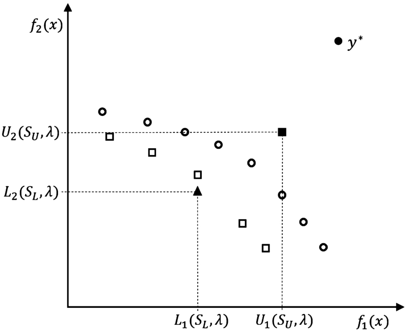
Given lower shell
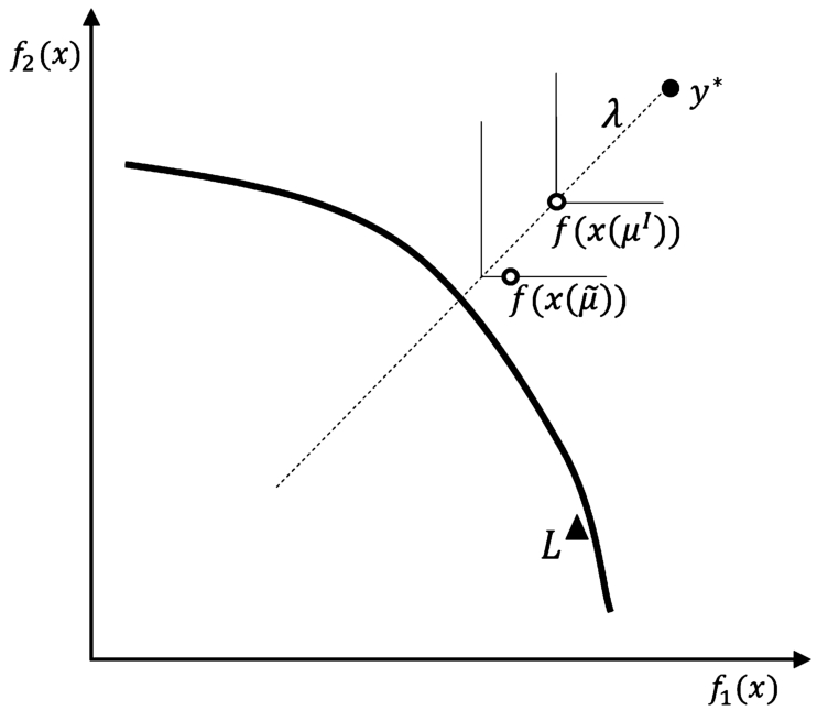
Let
Fig. 1
Components of
Further on,
3.1The Interval Representation of the Implicit Pareto Optimal Outcome
Given λ,
For
To gauge the quality of
(5)
4Providing Interval Representations of Implicit Pareto Optimal Outcomes
In this section, we develop a generic framework for providing interval representations of Pareto optimal outcomes, designated by weights of the Chebyshev scalarization, of the MOMIP problem when there is a time limit for optimization.
Given λ, we assume that there is a time limit
4.1The Derivation of Lower and Upper Shells
As in Kaliszewski and Miroforidis (2022), we will use
To populate upper shell
Lemma 2.
Given
Lemma 3.
If x is a Pareto optimal solution to the relaxation of problem (1) with
Given
The surrogate relaxation of problem (1) with
Given λ and
Fig. 2
Deriving upper shell
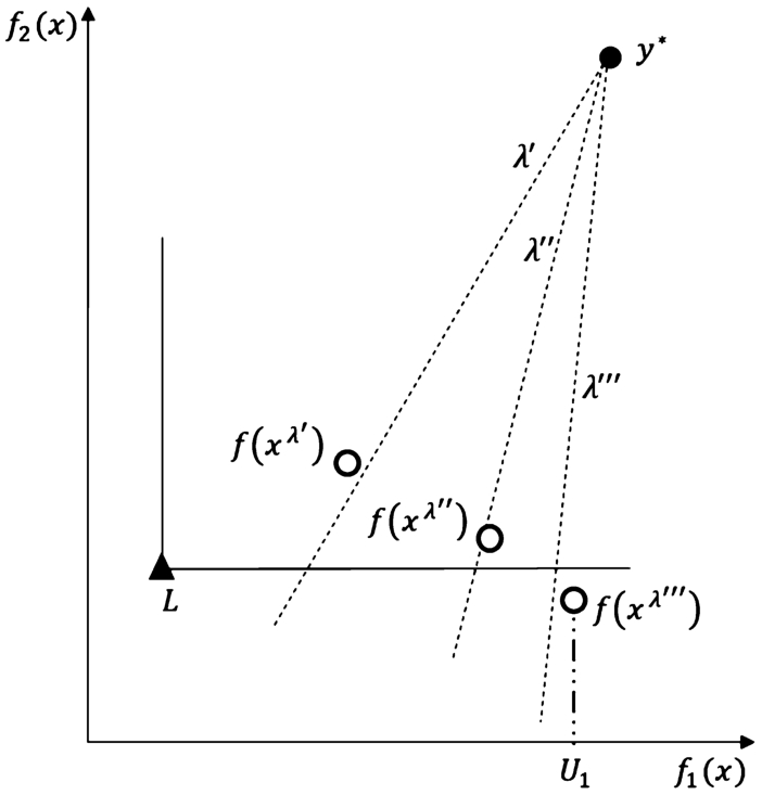
For
Iteration 1. We set the first probing vector
Iteration 2. We set
Iteration 3. We set
As elements
To obtain an upper bound on
Given
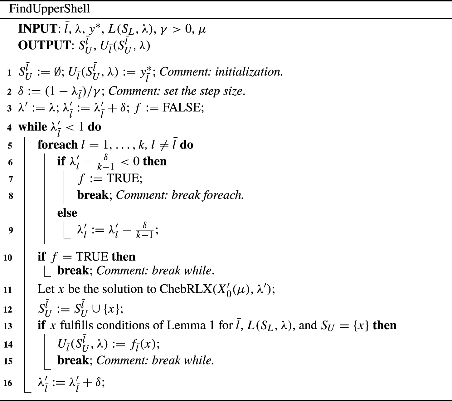
In Line 2, we set step size δ that is used to modify components of consecutive probing vectors
If no element of
4.2Calculating Interval Representations
Based on the above elements, an interval representation of the Pareto optimal outcome given by vector λ can be calculated with the use of the Chute algorithm. Along with the interval representation, this algorithm also returns lower and upper shells that were determined during its operation. In Section 5.7, we explain why the algorithm also returns lower and upper shells.
Line 4 of the algorithm needs clarification. Vector μ can be set as shown in Kaliszewski and Miroforidis (2022), namely by taking
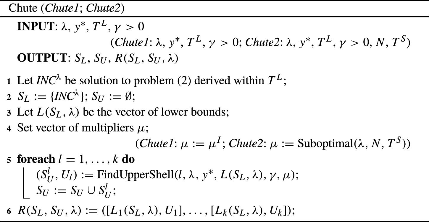
Yet, in Kaliszewski and Miroforidis (2022), in the section “Final remarks”, it has been suggested that “Tighter bounds might be obtained with other values of the multipliers. This possibility is worth exploring in future works.”. Unfortunately, there is no idea there how to select a vector of surrogate multipliers other than
Given μ, λ, let x be the solution to
Given λ, the best (highest) lower bound
(6)
“Number of iterations without improving the value of the objective function in problem (6) is greater than N” OR “time limit on optimization is greater than
In the current work, we set time limits on computation, hence the above stopping condition is justified in practice.
We will use vector
We shall call a version of the Chute algorithm that uses (in Line 4) the Suboptimal algorithm to set vector of surrogate multipiers μ for a given λ Chute2. It has two additional input parameters N and
Let us note that in the Chute2 algorithm, we set the vector of surrogate multipliers once for a given λ. The FindUpperShell algorithm uses perturbations of the λ vector to sample the objective space, and for all these perturbations the same vector μ is used. It is our heuristic assumption that even using the same vector μ for various vectors
Fig. 3
The idea of deriving upper shell
The idea (for
5Computational Experiments
In this section, we present the results of two experiments where we apply algorithms Chute1 and Chute2 presented in Section 4.2 to selected instances of the Multi-Objective Multidimensional 0–1 Knapsack Problem (MOMKP) with two and three objective functions. The instances are demanding for modern MIP solvers.
5.1Multi-Objective Multidimensional 0–1 Knapsack Problem
For
(7)
5.2Test Instances of the MOMIP Problem
As tri-criteria instances of the MOMKP, we take two instances from Kaliszewski and Miroforidis (2022) that were generated based on the 1st problem of the 6th group (
By removing the third objective function of problem Three6.1, we create a bi-criteria instance called Bi6.1. Analogously, by removing the third objective function of problem Three9.1, we create a bi-criteria instance called Bi9.1.
Bi6.1, Bi9.1, Three6.1, and Three9.1 are our test instances of the MOMIP problem.11
5.3Experimental Setting
Gurobi (version 10.0.0) for Microsoft Windows (x64) is our selected MIP solver. The optimizer is installed on the Intel Core i7-7700HQ-based laptop with 16 GB RAM.
To be consistent with limiting optimization time, we do not derive element
Table 1
Vectors λ and lower bounds for test problems Bi6.1 and Bi9.1.
| No. | λ | |||||
| 1 | 0.055 | 0.945 | 114253.29 | 130251.56 | 104466.45 | 118482.17 |
| 2 | 0.116 | 0.884 | 116707.61 | 129508.69 | 107215.43 | 117756.82 |
| 3 | 0.733 | 0.267 | 125690.15 | 122399.79 | 116288.83 | 110899.20 |
| 4 | 0.397 | 0.603 | 122075.81 | 126638.06 | 112806.06 | 115033.24 |
| 5 | 0.439 | 0.561 | 122514.80 | 126139.05 | 113385.01 | 114671.51 |
We set
For instances Bi6.1 and Bi9.1, we generate one set of five vectors λ uniformly sampled from two-dimensional unit simplex (see Smith and Tromble, 2004), and obtain corresponding vectors of lower bounds
Table 2
Vectors λ and lower bounds
| No. | λ | |||||
| 1 | 0.187 | 0.770 | 0.043 | 118622.54 | 128616.78 | 87944.84 |
| 2 | 0.521 | 0.324 | 0.155 | 124156.03 | 123541.43 | 115957.65 |
| 3 | 0.067 | 0.680 | 0.253 | 90480.66 | 127282.50 | 121460.00 |
| 4 | 0.359 | 0.295 | 0.346 | 120988.48 | 121527.94 | 123559.14 |
| 5 | 0.136 | 0.078 | 0.786 | 115623.82 | 108141.30 | 129431.77 |
Table 3
Vectors λ and lower bounds
| No. | λ | |||||
| 1 | 0.351 | 0.351 | 0.298 | 111876.06 | 111861.18 | 109288.07 |
| 2 | 0.243 | 0.143 | 0.614 | 110262.24 | 103915.65 | 114504.59 |
| 3 | 0.278 | 0.494 | 0.228 | 110549.31 | 114387.77 | 107363.36 |
| 4 | 0.179 | 0.471 | 0.350 | 105139.63 | 113934.39 | 110819.31 |
| 5 | 0.407 | 0.014 | 0.579 | 112514.84 | 0.00 | 113292.80 |
For all problem instances, for no vector λ, the selected MIP solver derived the solution to problem (2) in the assumed
We conduct two numerical experiments. In experiment 1, we test the behaviour of algorithm Chute1. In experiment 2, we test the behaviour of algorithm Chute2. In both experiments, on generated test instances, we test the behaviour of the Chute algorithm for
In the tables with results of the experiments, the meaning of the columns is as follows.
•
•
•
• Time
In bold, we indicate the improvement of a single component of
5.4Experiment 1 – Deriving Interval Representations with the Chute1 Algorithm
In this experiment, we check the behaviour of the Chute1 algorithm.
Table 4
Chute1, vectors of upper bounds for test problem Bi6.1 and
| No. | ||||||
| 1 | 120964.00 | 131117.00 | 120466.00 | 131117.00 | 120093.00 | 131117.00 |
| 2 | 121666.00 | 131117.00 | 121666.00 | 131117.00 | 121441.00 | 131117.00 |
| 3 | 127790.00 | 126078.00 | 127635.00 | 125842.00 | 127646.00 | 125642.00 |
| 4 | 125252.00 | 128990.00 | 124924.00 | 128990.00 | 124852.00 | 128990.00 |
| 5 | 125502.00 | 128779.00 | 125335.00 | 128665.00 | 125307.00 | 128710.00 |
Table 5
Chute1,
| No. | ||||||
| 1 | 5.55 | 0.66 | 5.16 | 0.66 | 4.86 | 0.66 |
| 2 | 4.08 | 1.23 | 4.08 | 1.23 | 3.90 | 1.23 |
| 3 | 1.64 | 2.92 | 1.52 | 2.74 | 1.53 | 2.58 |
| 4 | 2.54 | 1.82 | 2.28 | 1.82 | 2.22 | 1.82 |
| 5 | 2.38 | 2.05 | 2.25 | 1.96 | 2.23 | 2.00 |
Table 6
Chute1, values of
| No. | Time | |||||
| 1 | 11 | 32 | 52 | 1.90 | 8.00 | 11.49 |
| 2 | 11 | 33 | 54 | 2.02 | 5.97 | 11.52 |
| 3 | 8 | 21 | 34 | 2.07 | 4.26 | 9.12 |
| 4 | 7 | 19 | 31 | 2.38 | 5.90 | 9.50 |
| 5 | 7 | 19 | 32 | 2.08 | 5.63 | 8.59 |
Table 7
Chute1, vectors of upper bounds for test problem Bi9.1 and
| No. | ||||||
| 1 | 116289.00 | 119365.00 | 116289.00 | 119365.00 | 116193.00 | 119365.00 |
| 2 | 117277.00 | 119365.00 | 117050.00 | 119365.00 | 117057.00 | 119365.00 |
| 3 | 119379.88 | 118456.00 | 119379.88 | 118456.00 | 119379.88 | 118404.00 |
| 4 | 119379.88 | 119365.00 | 119295.00 | 119365.00 | 119329.00 | 119365.00 |
| 5 | 119379.88 | 119365.00 | 119379.88 | 119365.00 | 119379.88 | 119365.00 |
The results for instance Bi6.1 are shown in Tables 4–6, and the results for instance Bi9.1 are shown in Tables 7–9. The results for instance Three6.1 are shown in Tables 10–12, and the results for instance Three9.1 are shown in Tables 13–15.
Table 8
Chute1,
| No. | ||||||
| 1 | 10.17 | 0.74 | 10.17 | 0.74 | 10.09 | 0.74 |
| 2 | 8.58 | 1.35 | 8.40 | 1.35 | 8.41 | 1.35 |
| 3 | 2.59 | 6.38 | 2.59 | 6.38 | 2.59 | 6.34 |
| 4 | 5.51 | 3.63 | 5.44 | 3.63 | 5.47 | 3.63 |
| 5 | 5.02 | 3.93 | 5.02 | 3.93 | 5.02 | 3.93 |
Table 9
Chute1, values of
| No. | Time | |||||
| 1 | 12 | 36 | 59 | 3.06 | 11.22 | 20.44 |
| 2 | 14 | 40 | 67 | 3.91 | 10.70 | 17.21 |
| 3 | 17 | 51 | 84 | 3.82 | 13.05 | 21.78 |
| 4 | 20 | 59 | 99 | 59 | 13.79 | 24.32 |
| 5 | 20 | 60 | 100 | 60 | 14.84 | 21.51 |
Table 10
Chute1, vectors of upper bounds for test problem Three6.1 and
| No. | |||||||||
| 1 | 128872.00 | 131116.00 | 122914.00 | 128872.00 | 131116.00 | 122471.00 | 128872.00 | 131116.00 | 122387.00 |
| 2 | 127143.00 | 127325.00 | 124450.00 | 127069.00 | 127325.00 | 123193.00 | 127105.00 | 127325.00 | 122899.00 |
| 3 | 124359.00 | 131116.00 | 131738.00 | 124359.00 | 131116.00 | 131738.00 | 124217.00 | 131116.00 | 131738.00 |
| 4 | 125062.00 | 125714.00 | 126639.00 | 124809.00 | 125327.00 | 126342.00 | 124747.00 | 125273.00 | 126099.00 |
| 5 | 128872.00 | 120016.00 | 131738.00 | 128872.00 | 120016.00 | 131738.00 | 128872.00 | 119610.00 | 131738.00 |
Table 11
Chute1,
| No. | |||||||||
| 1 | 7.95 | 1.91 | 28.45 | 7.95 | 1.91 | 28.19 | 7.95 | 1.91 | 28.14 |
| 2 | 2.35 | 2.97 | 6.82 | 2.29 | 2.97 | 5.87 | 2.32 | 2.97 | 5.65 |
| 3 | 27.24 | 2.92 | 7.80 | 27.24 | 2.92 | 7.80 | 27.16 | 2.92 | 7.80 |
| 4 | 3.26 | 3.33 | 2.43 | 3.06 | 3.03 | 2.20 | 3.01 | 2.99 | 2.01 |
| 5 | 10.28 | 9.89 | 1.75 | 10.28 | 9.89 | 1.75 | 10.28 | 9.59 | 1.75 |
Table 12
Chute1, values
| No. | Time | |||||
| 1 | 8 | 14 | 33 | 2.69 | 4.46 | 10.48 |
| 2 | 11 | 21 | 50 | 3.39 | 7.80 | 23.98 |
| 3 | 11 | 21 | 49 | 5.37 | 11.84 | 22.38 |
| 4 | 7 | 12 | 28 | 5.46 | 9.28 | 24.29 |
| 5 | 11 | 21 | 51 | 3.27 | 6.54 | 16.37 |
Table 13
Chute1, vectors of upper bounds for test problem Three9.1 and
| No. | |||||||||
| 1 | 119379.88 | 119365.00 | 117516.00 | 119379.8835 | 119365.00 | 117398.00 | 119379.8835 | 119365.00 | 117362.00 |
| 2 | 119379.88 | 119365.00 | 118122.00 | 119379.8835 | 119365.00 | 118122.00 | 119379.8835 | 119365.00 | 118122.00 |
| 3 | 119379.88 | 119365.00 | 118122.00 | 119379.8835 | 119365.00 | 118122.00 | 119379.8835 | 119365.00 | 118122.00 |
| 4 | 119379.88 | 119365.00 | 118122.00 | 119379.8835 | 119365.00 | 118122.00 | 119379.8835 | 119365.00 | 118122.00 |
| 5 | 119379.88 | 119365.00 | 118122.00 | 119379.8835 | 119365.00 | 118122.00 | 119379.8835 | 119365.00 | 118122.00 |
Table 14
Chute1,
| No. | |||||||||
| 1 | 6.29 | 6.29 | 7.00 | 6.29 | 6.29 | 6.91 | 6.29 | 6.29 | 6.88 |
| 2 | 7.64 | 12.94 | 3.06 | 7.64 | 12.94 | 3.06 | 7.64 | 12.94 | 3.06 |
| 3 | 7.40 | 4.17 | 9.11 | 7.40 | 4.17 | 9.11 | 7.40 | 4.17 | 9.11 |
| 4 | 11.93 | 4.55 | 6.18 | 11.93 | 4.55 | 6.18 | 11.93 | 4.55 | 6.18 |
| 5 | 5.75 | 100.00 | 4.09 | 5.75 | 100.00 | 4.09 | 5.75 | 100.00 | 4.09 |
Table 15
Chute1, values of
| No. | Time | |||||
| 1 | 28 | 79 | 130 | 50.09 | 163.04 | 237.71 |
| 2 | 18 | 53 | 86 | 46.24 | 324.61 | 413.15 |
| 3 | 25 | 69 | 115 | 79.80 | 222.40 | 387.76 |
| 4 | 22 | 64 | 105 | 36.09 | 104.40 | 175.58 |
| 5 | 11 | 29 | 49 | 11.38 | 50.33 | 101.04 |
For instance Bi6.1, when changing
When changing
For instance Bi9.1, we observe a similar phenomenon (an improvement, as well as a deterioration), although when changing
For instances Bi6.1 and Bi9.1, the higher the value of parameter γ (higher sampling density of the objective space), the more numerous the derived upper shells are. For each vector λ, the time to derive the corresponding upper shell is a small fraction of the assumed time limit
Let us check the results for tri-criteria instances. For instance Three6.1, when changing
We checked that for all instances, for no vector λ, the MIP solver derived the optimal solution to problem (2) within time limit
5.5Experiment 2 – Deriving Interval Representations with the Chute2 Algorithm
In this experiment, we check the behaviour of the Chute2 algorithm with
The results for instance Bi6.1 are shown in Tables 16–18, and the results for instance Bi9.1 are shown in Tables 19–21. The results for instance Three6.1 are shown in Tables 22–24, and the results for instance Three9.1 are shown in Tables 25–27.
Table 16
Chute2, upper bounds for test problem Bi6.1 and
| No. | ||||||
| 1 | 118423.00 | 130703.00 | 116671.00 | 130703.00 | 116230.00 | 130703.00 |
| 2 | 119507.00 | 130021.00 | 118226.00 | 129980.00 | 117969.00 | 129946.00 |
| 3 | 126391.00 | 123927.00 | 126213.00 | 123235.00 | 126179.00 | 123296.00 |
| 4 | 123079.00 | 127228.00 | 122598.00 | 127102.00 | 122657.00 | 127146.00 |
| 5 | 123474.00 | 126864.00 | 123273.00 | 126864.00 | 123233.00 | 126766.00 |
Table 17
Chute2,
| No. | ||||||
| 1 | 3.52 | 0.35 | 2.07 | 0.35 | 1.70 | 0.35 |
| 2 | 2.34 | 0.39 | 1.28 | 0.36 | 1.07 | 0.34 |
| 3 | 0.55 | 1.23 | 0.41 | 0.68 | 0.39 | 0.73 |
| 4 | 0.82 | 0.46 | 0.43 | 0.37 | 0.47 | 0.40 |
| 5 | 0.78 | 0.57 | 0.62 | 0.57 | 0.58 | 0.49 |
Table 18
Chute2,
| No. | Time | |||||
| 1 | 6 | 16 | 26 | 81.16 (78.64) | 84.79 (77.97) | 91.44 (79.81) |
| 2 | 4 | 9 | 13 | 182.12 (180.58) | 215.77 (211.45) | 197.74 (192.33) |
| 3 | 3 | 5 | 8 | 37.59 (36.74) | 41.65 (38.50) | 42.82 (37.99) |
| 4 | 2 | 3 | 6 | 42.39 (41.04) | 41.65 (40.42) | 44.57 (41.78) |
| 5 | 2 | 5 | 7 | 44.07 (43.33) | 41.28 (39.66) | 39.82 (37.83) |
Table 19
Chute2, upper bounds for test problem Bi9.1 and
| No. | ||||||
| 1 | 110646.00 | 119365.00 | 109109.00 | 119365.00 | 109313.00 | 119365.00 |
| 2 | 111592.00 | 119218.00 | 111080.00 | 119124.00 | 110985.00 | 119105.00 |
| 3 | 118331.00 | 114263.00 | 118172.00 | 113760.00 | 118138.00 | 113655.00 |
| 4 | 115241.00 | 116795.00 | 115230.00 | 116781.00 | 115121.00 | 116732.00 |
| 5 | 115443.00 | 116518.00 | 115426.00 | 116271.00 | 115321.00 | 116233.00 |
Table 20
Chute2,
| No. | ||||||
| 1 | 5.58 | 0.74 | 4.25 | 0.74 | 4.43 | 0.74 |
| 2 | 3.92 | 1.23 | 3.48 | 1.15 | 3.40 | 1.13 |
| 3 | 1.73 | 2.94 | 1.59 | 2.51 | 1.57 | 2.42 |
| 4 | 2.11 | 1.51 | 2.10 | 1.50 | 2.01 | 1.46 |
| 5 | 1.78 | 1.58 | 1.77 | 1.38 | 1.68 | 1.34 |
Table 21
Chute2,
| No. | Time | |||||
| 1 | 11 | 31 | 52 | 439.96 (411.14) | 515.48 (402.94) | 665.55 (404.57) |
| 2 | 10 | 27 | 44 | 482.23 (407.04) | 678.38 (402.56) | 765.19 (409.44) |
| 3 | 8 | 20 | 32 | 443.50 (406.40) | 534.97 (410.38) | 667.23 (404.69) |
| 4 | 5 | 15 | 23 | 424.95 (403.06) | 465.13 (400.30) | 484.92 (402.56) |
| 5 | 5 | 13 | 20 | 432.90 (400.51) | 485.67 (404.07) | 512.03 (403.40) |
For instance Bi6.1, when changing
Table 22
Chute2, upper bounds for test problem Three6.1 and
| No. | |||||||||
| 1 | 128872.00 | 131116.00 | 122259.00 | 128872.00 | 131116.00 | 120988.00 | 128872.00 | 131116.00 | 120434.00 |
| 2 | 125477.00 | 125196.00 | 121464.00 | 125483.00 | 125196.00 | 120230.00 | 125477.00 | 125196.00 | 119034.00 |
| 3 | 122652.00 | 131116.00 | 131738.00 | 122094.00 | 131116.00 | 131738.00 | 122334.00 | 131116.00 | 131738.00 |
| 4 | 122671.00 | 123772.00 | 125154.00 | 122242.00 | 123201.00 | 124765.00 | 122404.00 | 123097.00 | 124677.00 |
| 5 | 128872.00 | 119155.00 | 131738.00 | 128872.00 | 118229.00 | 131738.00 | 128872.00 | 117837.00 | 131738.00 |
Table 23
Chute2,
| No. | |||||||||
| 1 | 7.95 | 1.91 | 28.07 | 7.95 | 1.91 | 27.31 | 7.95 | 1.91 | 26.98 |
| 2 | 1.05 | 1.32 | 4.53 | 1.06 | 1.32 | 3.55 | 1.05 | 1.32 | 2.58 |
| 3 | 26.23 | 2.92 | 7.80 | 25.89 | 2.92 | 7.80 | 26.04 | 2.92 | 7.80 |
| 4 | 1.37 | 1.81 | 1.27 | 1.03 | 1.36 | 0.97 | 1.16 | 1.27 | 0.90 |
| 5 | 10.28 | 9.24 | 1.75 | 10.28 | 8.53 | 1.75 | 10.28 | 8.23 | 1.75 |
Table 24
Chute2,
| No. | Time | |||||
| 1 | 8 | 20 | 31 | 106.30 (104.24) | 133.88 (121.32) | 118.75 (102.00) |
| 2 | 4 | 11 | 17 | 413.24 (408.25) | 436.70 (409.23) | 429.80 (401.94) |
| 3 | 10 | 27 | 44 | 50.87 (47.43) | 76.35 (61.08) | 60.59 (41.18) |
| 4 | 3 | 6 | 10 | 293.45 (289.56) | 380.25 (365.56) | 353.60 (319.88) |
| 5 | 11 | 30 | 50 | 56.90 (51.22) | 66.93 (51.58) | 79.55 (50.46) |
Table 25
Chute2, upper bounds for test problem Three9.1 and
| No. | |||||||||
| 1 | 115765.00 | 115804.00 | 113089.00 | 115250.00 | 115546.00 | 112742.00 | 115126.00 | 115335.00 | 112656.00 |
| 2 | 114092.00 | 113121.00 | 118122.00 | 113842.00 | 112477.00 | 117089.00 | 113861.00 | 112778.00 | 118122.00 |
| 3 | 116240.00 | 117966.00 | 112426.00 | 116229.00 | 117577.00 | 111977.00 | 116160.00 | 117657.00 | 111578.00 |
| 4 | 112893.00 | 116633.00 | 114061.00 | 112291.00 | 116382.00 | 113713.00 | 112177.00 | 116438.00 | 113665.00 |
| 5 | 119379.88 | 112286.00 | 118122.00 | 119379.88 | 111440.00 | 118122.00 | 119379.88 | 111242.00 | 118122.00 |
Table 26
Chute2,
| No. | |||||||||
| 1 | 3.36 | 3.40 | 3.36 | 2.93 | 3.19 | 3.06 | 2.82 | 3.01 | 2.99 |
| 2 | 3.36 | 8.14 | 3.06 | 3.14 | 7.61 | 2.21 | 3.16 | 7.86 | 3.06 |
| 3 | 4.90 | 3.03 | 4.50 | 4.89 | 2.71 | 4.12 | 4.83 | 2.78 | 3.78 |
| 4 | 6.87 | 2.31 | 2.84 | 6.37 | 2.10 | 2.54 | 6.27 | 2.15 | 2.50 |
| 5 | 5.75 | 100.00 | 4.09 | 5.75 | 100.00 | 4.09 | 5.75 | 100.00 | 4.09 |
Table 27
Chute2,
| No. | Time | |||||
| 1 | 8 | 20 | 31 | 519.63 (420.77) | 548.70 (400.11) | 654.78 (411.71) |
| 2 | 12 | 32 | 55 | 412.71 (403.34) | 478.80 (409.01) | 521.99 (401.65) |
| 3 | 12 | 32 | 52 | 444.12 (400.92) | 527.00 (404.25) | 605.74 (405.75) |
| 4 | 9 | 22 | 36 | 425.02 (400.11) | 462.81 (405.86) | 515.93 (405.72) |
| 5 | 5 | 12 | 20 | 325.93 (323.31) | 335.62 (324.23) | 360.17 (330.95) |
For instance Bi9.1, when changing
For instances Bi6.1 and Bi9.1, the higher the value of parameter γ (higher sampling density of the objective space), the more numerous the derived upper shells are. For instance Bi6.1, average times over all vectors λ to derive the upper shell for
Let us check the results for tri-criteria instances. For instance Three6.1, when changing
For instance Three9.1, when changing
For instances Three6.1 and Three9.1, the higher the value of parameter γ (higher sampling density of the objective space), the more numerous the derived upper shells are. For instance Three9.1, average times over all vectors λ to derive the upper shell for
We checked that for all instances, for no vector λ, the MIP solver derived the optimal solution to problem (2) within time limit
5.6Comparing Chute2 with Chute1
When comparing Chute2 to Chute1, for all tested instances and all values of the γ parameter, we observe no deterioration of any component of
For instance Bi6.1, for all values of γ, all components of
For instance Bi9.1, for
For instance Three6.1, for
For instance Three9.1, for all γ, at least one component of
Table 28 shows times of deriving upper shells averaged over all vectors λ for both tested algorithms. We observe a significant increase in these times for Chute2 compared to Chute1. It should be recalled here that Chute2 uses the Suboptimal algorithm, for which the stopping condition depends on the assumed for this algorithm time limit
Table 28
Average times of deriving upper shells for Chute1 and Chute2.
| γ | AVG Time | AVG Time |
| Chute1 | Chute2 | |
| Bi6.1 | ||
| 10 | 2.09 | 77.47 (76.07) |
| 30 | 5.95 | 85.03 (81.60) |
| 50 | 10.04 | 83.28 (77.95) |
| Bi9.1 | ||
| 10 | 4.02 | 444.71 (405.63) |
| 30 | 12.72 | 535.92 (404.05) |
| 50 | 21.05 | 618.98 (404.93) |
| Three6.1 | ||
| 10 | 4.04 | 184.15 (180.14) |
| 30 | 7.98 | 218.82 (201.75) |
| 50 | 19.50 | 208.46 (183.09) |
| Three9.1 | ||
| 10 | 44.72 | 425.48 (389.69) |
| 30 | 172.96 | 470.58 (388.69) |
| 50 | 263.05 | 531.72 (391.16) |
5.7Discussion
For all test instances of the MOMIP problem, with time limits set, algorithm Chute2 determines tighter upper bounds measured with the help of
The deterioration of some of the components of
Parameters affecting the operation of algorithms Chute1 and Chute2 (in particular, time limits for optimization, as well as parameter γ) were arbitrarily set for the numerical experiments conducted on the selected test instances. We can not recommend the adopted parameter values (e.g.
As Chute1 and Chute2 use a MIP solver as a black box, it is difficult to provide their theoretical performance, especially since they can work with any instance of the MOMIP problem that meets the very generic assumptions made in this work. During their operation, multiple instances of the single-objective MIP problem are solved, which are parameterized by λ in the case of Chute1 and (
The Chute algorithm returns not only the interval representation but also lower and upper shells. Let us assume that for a given set
Fig. 4
A finite two-sided approximation of the Pareto front: □, ∘ – images of lower shell
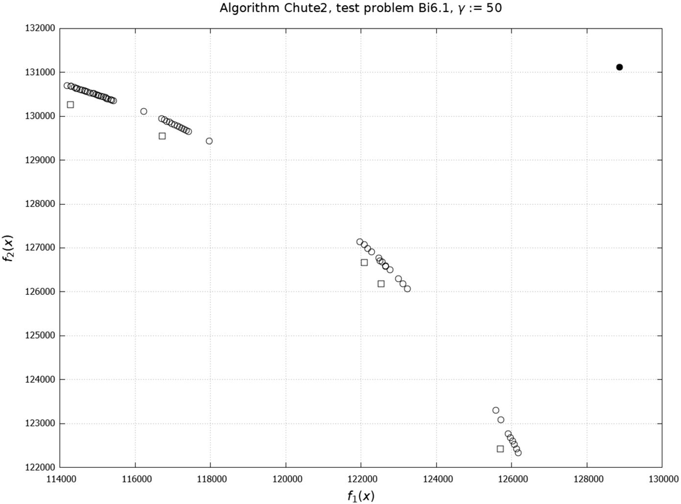
We can say that we obtained the two-sided approximation of the Pareto front, shaped by the DM’s preferences expressed with the help of vectors λ.
Although we aim not to derive approximations of the entire Pareto front (as in multi-objective branch and bound, see, e.g. Przybylski and Gandibleux, 2017; Forget et al., 2022) for
6Limitations of the Chute Algorithm and Its Possible Enhancements
In this section, we discuss the limitations and possible enhancements of the Chute algorithm to better adapt it to the realities of decision-making and the budgeting of calculations.
In the Chute algorithm, we have assumed that for all probing vectors
However, one can imagine version Chute3 of the Chute algorithm in which the determination of vector μ takes place in the FindUpperShell algorithm for each probing
In a real decision-making process using the Chute algorithm, it is possible to calculate a more adjusted value of parameter γ for a new vector λ based on the properties of the lower and upper shells obtained for previous vectors λ, and with which this algorithm was called. Let us look, for example, at Table 18. For
In the proposed method of deriving upper shells (algorithm FindUpperShell), there is no single parameter to limit optimization time for getting theirs. Yet, such a time limit can be incorporated relatively easily as an additional stop condition in FindUpperShell. More generally, it could be even desirable to introduce in the Chute algorithm a time limit for determining the interval representation of the implicit Pareto optimal outcome for a given vector λ. The DM would give, for example, in addition to λ and
Based on the above alone, one can imagine many schemes for budgeting calculations, leading to providing interval representations in a decision-making system based on the Chute algorithm.
In our approach, to find elements of the upper shell we solve to optimality the Chebyshev scalarization of the surrogate relaxation of the MOMIP problem. For instances of the MOMIP problem with a large number of constraints (e.g. 1000), even with a suboptimal vector of multipliers μ provided by the Suboptimal algorithm (that is, with a single constraint that mimics the original set of constraints of the MOMIP problem), the FindUpperShell procedure may not derive elements x of the upper shell that
To find (sub)optimal values of multipliers
Within the generic framework presented, other methods of deriving upper shells in the FindUpperShell procedure can also be applied, e.g. a method shown in Miroforidis (2021).
7Final Remarks
It has been shown how to algorithmically derive lower and upper shells to the MOMIP problem (for any
We conducted some preliminary experiments with the Chute algorithm on instances of the MOMKP with four objective functions. However, due to the mechanism adopted in the FindUpperShell algorithm for changing the probing λ vectors, the results achieved were not satisfactory.
In our future work, we want to improve the method of populating upper shells (in quest of finding their elements that can provide upper bounds) by changing the scheme of probing the objective space. We want it to determine upper shells with the desired properties for four and more objective functions. We also want to apply the presented generic approach to other instances of the MOMIP problem, especially ones connected to real-life problems. This would help verify the practicality of the proposed general method and identify those elements that could be tailored for specific instances of this problem. Possible modifications to the proposed method are indicated in Section 6. These are also worth considering in further work.
Notes
1 The instances can be made available to the reader by e-mail upon request.
Acknowledgements
We thank two anonymous reviewers for their helpful comments.
References
1 | Ahmadi, A., Aghaei, J., Shayanfar, H.A., Rabiee, A. ((2012) ). Mixed integer programming of multiobjective hydro-thermal self scheduling. Applied Soft Computing, 12: , 2137–2146. https://doi.org/10.1016/j.asoc.2012.03.020. |
2 | Delorme, X., Battaïa, O., Dolgui, A. ((2014) ). Multi-objective approaches for design of assembly lines. In: Benyoucef, L., Hennet, C., J., Tiwari, M. (Eds.), Applications of Multi-Criteria and Game Theory Approaches: Manufacturing and Logistics. Springer, London, pp. 31–56. https://doi.org/10.1007/978-1-4471-5295-8_2. |
3 | Dyer, M.E. ((1980) ). Calculating Surrogate Constraints. Mathematical Programming, 19: , 255–278. https://doi.org/10.1007/BF01581647. |
4 | Ehrgott, M. ((2005) ). Multicriteria Optimization. Springer, Berlin, Heidelberg. https://doi.org/10.1007/3-540-27659-9. |
5 | Eiselt, H.A., Marianov, V. ((2014) ). A bi-objective model for the location of landfills for municipal solid waste. European Journal of Operational Research, 235: 1, 187–194. https://doi.org/10.1016/j.ejor.2013.10.005. |
6 | Forget, N., Gadegaard, S.L., Klamroth, K., Nielsen, L.R., Przybylski, A. ((2022) ). Branch-and-bound and objective branching with three or more objectives. Computers & Operations Research, 148: , 106012. https://doi.org/10.1016/j.cor.2022.106012. |
7 | Glover, F. ((1965) ). A multiphase-dual algorithm for the zero-one integer programming problem. Operations Research, 13: (6), 879–919. https://doi.org/10.1287/opre.13.6.879. |
8 | Glover, F. ((1968) ). Surrogate constraints. Operations Research, 16: 4, 741–749. https://doi.org/10.1287/opre.16.4.741. |
9 | Gurobi (2023). GUROBI. Last accessed March 31, 2023. https://www.gurobi.com/. |
10 | IBM (2023). CPLEX. Last accessed March 31, 2023. https://www.ibm.com/products/ilog-cplex-optimization-studio. |
11 | Kaliszewski, I. ((2006) ). Soft Computing for Complex Multiple Criteria Decision Making. Springer, New York. https://doi.org/10.1007/0-387-30177-1. |
12 | Kaliszewski, I., Miroforidis, J. ((2014) ). Two-sided Pareto front approximations. Journal of Optimization Theory and Its Applications, 162: , 845–855. https://doi.org/10.1007/s10957-013-0498-y. |
13 | Kaliszewski, I., Miroforidis, J. ((2019) ). Lower and upper bounds for the general multiobjective optimization problem. AIP Conference Proceedings, 2070: , 020038. https://doi.org/10.1063/1.5090005. |
14 | Kaliszewski, I., Miroforidis, J. ((2021) ). Cooperative multiobjective optimization with bounds on objective functions. Journal of Global Optimization, 79: , 369–385. https://doi.org/10.1007/s10898-020-00946-4. |
15 | Kaliszewski, I., Miroforidis, J. ((2022) ). Probing the Pareto front of a large-scale multiobjective problem with a MIP solver. Operational Research, 22: , 5617–5673. https://doi.org/10.1007/s12351-022-00708-y. |
16 | Kaliszewski, I., Miroforidis, J., Podkopaev, D. ((2016) ). Multiple Criteria Decision Making by Multiobjective Optimization – A Toolbox. Springer Cham. https://doi.org/10.1007/978-3-319-32756-3. |
17 | Miettinen, K.M. ((1999) ). Nonlinear Multiobjective Optimization. Kluwer Academic Publishers. https://doi.org/10.1007/978-1-4615-5563-6. |
18 | Miroforidis, J. ((2021) ). Bounds on efficient outcomes for large-scale cardinality-constrained Markowitz problems. Journal of Global Optimization, 80: , 617–634. https://doi.org/10.1007/s10898-021-01022-1. |
19 | Narciso, M.G., Lorena, L.A.N. ((1999) ). Lagrangean/surrogate relaxation for generalized assignment problems. European Journal of Operational Research, 114: (1), 165–177. https://doi.org/10.1016/S0377-2217(98)00038-1. |
20 | Oke, O., Siddiqui, S. ((2015) ). Efficient automated schematic map drawing using multiobjective mixed integer programming. Computers & Operations Research, 61: , 1–17. https://doi.org/10.1016/j.cor.2015.02.010. |
21 | Przybylski, A., Gandibleux, X. ((2017) ). Multi-objective branch and bound. European Journal of Operational Research, 260: (3), 856–872. https://doi.org/10.1016/j.ejor.2017.01.032. |
22 | Samanlioglu, F. ((2013) ). A multi-objective mathematical model for the industrial hazardous waste location-routing problem. European Journal of Operational Research, 226: (2), 332–340. https://doi.org/10.1016/j.ejor.2012.11.019. |
23 | Sikorski, J. ((1986) ). Quasi–Subgradient algorithms for calculating surrogate constraints. In: Malanowski, K., Mizukami, K. (Eds.), Analysis and Algorithms of Optimization Problems, Lecture Notes in Control and Information Sciences, Vol. 82: . Springer Berlin Heidelberg, Berlin, Heidelberg, pp. 202–236. https://doi.org/10.1007/BFb0007163. |
24 | Smith, N.A., Tromble, R.W. ((2004) ). Sampling Uniformly from the Unit Simplex. Department of Computer Science, Center for Language and Speech Recognition, Johns Hopkins University. |


