
An Extended EDAS Approach Based on Cumulative Prospect Theory for Multiple Attributes Group Decision Making with Interval-Valued Intuitionistic Fuzzy Information
Abstract
The interval-valued intuitionistic fuzzy sets (IVIFSs), based on the intuitionistic fuzzy sets (IFSs), combine the classical decision method and its research and application is attracting attention. After a comparative analysis, it becomes clear that multiple classical methods with IVIFSs’ information have been applied to many practical issues. In this paper, we extended the classical EDAS method based on the Cumulative Prospect Theory (CPT) considering the decision experts (DEs)’ psychological factors under IVIFSs. Taking the fuzzy and uncertain character of the IVIFSs and the psychological preference into consideration, an original EDAS method, based on the CPT under IVIFSs (IVIF-CPT-EDAS) method, is created for multiple-attribute group decision making (MAGDM) issues. Meanwhile, the information entropy method is used to evaluate the attribute weight. Finally, a numerical example for Green Technology Venture Capital (GTVC) project selection is given, some comparisons are used to illustrate the advantages of the IVIF-CPT-EDAS method and a sensitivity analysis is applied to prove the effectiveness and stability of this new method.
1Introduction
During the long history of humanity, conflicts between environmental issues and economic growth have always been one of the key issues (Yang et al., 2022) discussed by various researchers. Especially after the Industrial Revolution, while human society greatly improved production efficiency and promoted economic development, the environmental pollution caused by industrial production and manufacturing also constantly threatened human health and survival. Therefore, in order to ensure stable economic development, we should seek a more long-term and sustainable development path. Specifically, the GTVC (Dong et al., 2021; Dhayal et al., 2023), created by integrating the concept of green development into the traditional financial system, is in line with the demand. It is an emerging project technology related to protecting and improving the environment. In the processes of GTVC, project screening and evaluation are important. However, project evaluation often involves many qualitative indicators, coupled with the cognitive limitations of DEs and the complexity of actual decision making (DM) scenarios, which may lead to significant ambiguity in input information.
On the other hand, multiple criteria decision-making (MCDM) is usually classified (Hashemi-Tabatabaei et al., 2019; Keshavarz-Ghorabaee, 2021; Keshavarz-Ghorabaee et al., 2018, 2021, 2016) into two categories: multiple attribute decision-making (MADM) (Ning et al., 2022; Zhang et al., 2021) and multiple objective decision-making (MODM), based on whether the DM scheme is finite or infinite. MODM refers to the DM problem that only considers two or more objectives simultaneously. MADM, also known as finite alternative MODM, refers to the decision problem of selecting the optimal alternative solution considering multiple attributes. MAGDM is an important component of modern decision science, as it integrates the advantages of MADM and group DM (GDM). Currently, the relative theories and methods on MAGDM (Y. Li et al., 2021; Ning et al., 2023; Zhang et al., 2023) are widely applied in fields such as investment risk and economic management. Moreover, MAGDM technology can utilize a systematic and logical approach to collect and process multidimensional fuzzy evaluation information to determine the best alternative.
That being the case, it is necessary to design a suitable and advanced MAGDM model in a fuzzy environment to select the optimal GTVC project. To enhance the readability of the proposed research work, we have sorted out some important abbreviations, as shown in Table 1.
Table 1
Description of abbreviations.
| Abbreviations | Description |
| DE | Decision expert |
| DM | Decision making |
| FS | Fuzzy set |
| IFS | Intuitionistic fuzzy set |
| IVIFS | Interval valued intuitionistic fuzzy set |
| IVIFN | Interval valued intuitionistic fuzzy number |
| IVIFWA | Interval valued intuitionistic fuzzy weighted averaging |
| IVIFWG | Interval valued intuitionistic fuzzy geometric |
| SF | Score function |
| AF | Accuracy function |
| CPT | Cumulative prospect theory |
| GTVC | Green technology venture capital |
| PDA(NDA) | Positive (Negative) distance from average |
| MAGDM | Multiple attribute group decision making |
| CRITIC | CRiteria importance through intercriteria correlation |
| EDAS | Evaluation based on distance from average solution |
| TOPSIS | Technique for order preference by similarity to ideal solution |
| TODIM | An acronym in Portuguese for interactive and multicriteria decision making |
| MABAC | Muti-attributive border approximation area comparison |
1.1Motivations and Contributions for Proposed Research
The motivations of this study are given below:
(1) With the increasing complexity of DM problems and the ambiguity of informative data, DEs find it is difficult to accurately quantify their evaluations using single numerals, but their preferences can be expressed more completely in natural language. Linguistic IVIFS theory is one of the most effective generalizations in FS theory, which can describe the assessment information of DEs in even more detail.
(2) Compared with other evaluation methods, the EDAS method is a highly effective tool to execute classification and decision for contradictory attributes in MAGDM. Classical EDAS algorithms assume that all decision makers are perfectly rational, but people have different views on the same level of risks and benefits in practical environments. They are more conservative when facing equal risks than when facing returns. Therefore, it is necessary to develop a technology that simulates the real DM environment to model IVIF information and evaluate the weights of attributes. From this perspective, it is necessary to integrate the CPT, which takes the DEs’ risk preference into consideration, and the IVIF-EDAS method.
(3) Due to the fact that the entropy method determines attribute weights based on the degree of the indicator confusion, the higher the degree of indicator information confusion, the greater the entropy value, and the smaller the assigned weights. Combined with the advantages of the EDAS method in solving DM problems with conflicting attributes, it is necessary to extend the information entropy method to handle qualitative information in the IVIF environment to guarantee the stability of the entire DM system.
(4) As a key research issue in the MAGDM field, the selection of high-quality GTVC projects has a great significance for environmental protection and sustainable economic development. In this regard, considering the advantages of the EDAS method, the CPT’s characteristics and the IVIFSs which may contain more information, the aim of this paper is to extend the EDAS method based on CPT for MAGDM under IVIFSs and apply it to the GTVC project selection.
The contributions of this paper are as follows:
(1) The integration of CPT and the EDAS method in IVIFSs, named as the IVIF-CPT-EDAS method, is discussed to determine which GTVC project is suitable. The attribute weights are determined by using IVIF-entropy method and alternatives are ranked by using CPT-EDAS method in a IVIF context. Therefore, our proposed method combines DEs evaluation values which makes it more profitable to use and the decision results more precise.
(2) The IVIF-CPT-EDAS method, which considers not only the relatively simple and reasonable classical method, but also the psychological state of DEs, which is more realistic, has been constructed.
(3) We implement the constructed approach to a numerical example for GTVC project selection to demonstrate the applicability of our proposed methodology.
(4) We compare the constructed approach with the existing methods to illustrate the advantages of the IVIF-CPT-EDAS method. Furthermore, comparative analysis and sensitivity analysis are used to illustrate the effectiveness and authenticity of the developed approach.
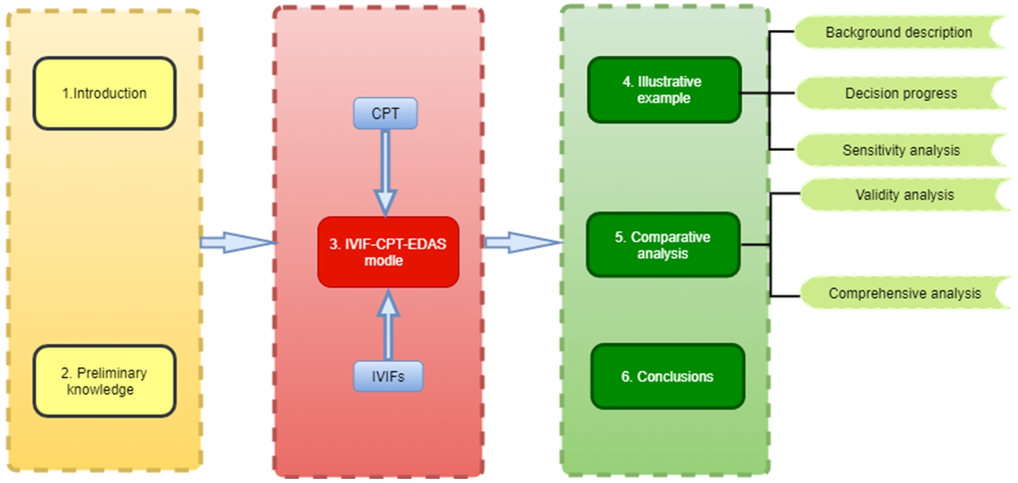
In order to do so, the overall structure of the article is as follows: the basic knowledge of IVIFSs is briefly introduced in Section 2, then the IVIF-CPT-EDAS method is constructed in Section 3. Section 4 gives a numerical study for GTVC project selection, and the corresponding parameters’ sensitivity, and in Section 5, a comparison analysis is made to prove its effectiveness and stability. In Section 6, conclusions are made to summarize this paper. Figure 1 represents the full framework of our study.
Fig. 1
Full text framework diagram.
1.2Literature Review
In most practical decisions, the DEs’ evaluation of an index cannot be simply expressed by real numbers (Ye, 2017; Liu and You, 2019; Gao et al., 2019a, 2019b). Therefore, Zadeh (1965) introduced fuzzy sets (FSs), and later this theory and its extensions have been applied to many fields (Zeng et al., 2018; Chen, 2018). An extension of the FSs, such as the IFSs (Atanassov, 1986), is the classical fuzzy set, and due to the fact that the IFSs are in the range of real numbers, the IVIFSs can extend the IFSs with the interval numbers to fully express different conditions of the DM. Atanassov and Gargov (1989) proposed the IVIFSs, and the corresponding operators (Atanassov, 1994), and with some basic research made, the corresponding innovation of IVIFSs has been proposed. Grzegorzewski (2004) proposed a new distance assessment based on Hausdorff metric which is the well-known Hamming distance. Based on some operational laws of IVIFSs, TOPSIS method (Lin et al., 2019; Yue and Zhang, 2020; Zulqarnain et al., 2021; Chen, 2015), Grey Relational Analysis method (Fankang et al., 2020; Hongjiu et al., 2019; Wei and Lan, 2008; Zhang and Wang, 2022), VIKOR method (Dammak et al., 2020; Salimian et al., 2022a; Wu et al., 2019), TODIM method (Krohling and Pacheco, 2014; Lin et al., 2020; Zhao et al., 2021; Zindani et al., 2021), MABAC method (Keshavarz-Ghorabaee et al., 2015; Liu et al., 2019; Mahmoudi et al., 2019; Salimian et al., 2022b), and other methods have been applied to the IVIFSs (Kumar and Chen, 2022; Li et al., 2012, 2021; Lee, 2009; Ye et al., 2021).
The EDAS method (Huang and Lin, 2021; Karunanithi et al., 2015; Keshavarz-Ghorabaee et al., 2015) assesses the alternatives by the positive (negative) distance from average (PDA and NDA). In other words, the higher value of the PDA or the lower value of the NDA means a more optimal alternative. Among numerous evaluation methods, EDAS not only has much easier formulas, but also has unique advantages in resolving conflicts between economic development and green technology evaluation elements, making it more efficient and accurate than others. On the one hand, the EDAS method has been applied to many fuzzy sets (Agrawal et al., 2023; Ecer et al., 2022; Zolfani et al., 2021), for instance, IFSs (Kahraman et al., 2017), interval-valued fuzzy soft sets (Peng et al., 2017), hesitant fuzzy linguistic sets (Feng et al., 2018), interval-valued neutronsophic sets (Karasan and Kahraman, 2018), and so on. On the other hand, it can be seen that the EDAS method has good adaptability in the DM fields. Dinghong and Wenhua (2021) applied the EDAS method to the selection of smart zero waste cities, and Mishra et al. (2020) applied the EDAS method to the selection of medical waste treatment technologies. Although Li and Wang (2020) extended the EDAS method to IVIFSs, this model cannot take the risk reference of DEs into consideration. Due to the fact that most methods are based on the utility theory which considers that DEs are entirely rational, the combination of CPT (Tversky and Kahneman, 1992) and the classical EDAS method are now applied to some FSs, such as probabilistic hesitant fuzzy sets (Liao et al., 2023) and picture fuzzy sets (Jiang et al., 2022). We discussed some important previously proposed models and methods in Table 2 to highlight the superiority of our study.
Table 2
Characteristic table of different approaches.
| Year | Approach | Linguistic data | Fuzzy information form | Application |
| 2012 | IVIF-TOPSIS (Izadikhah, 2012) | ✓ | Intuitionistic fuzzy number | Supplier selection |
| 2018 | EHFLTS-EDAS (Feng et al., 2018) | ✓ | Hesitant fuzzy linguistic term set | Company project selection |
| 2019 | IVIF-VIKOR (Wu et al., 2019) | ✕ | Interval-valued intuitionistic fuzzy set | Financing risk assessment |
| 2020 | IVIF-EDAS (Li and Wang, 2020) | ✕ | Intuitionistic fuzzy number | Computer network system assessment |
| 2022 | F-SECA (Keshavarz-Ghorabaee et al., 2022) | ✓ | Triangular fuzzy numbers | E-waste scenario evaluation |
| 2022 | F-SBWM (Amiri et al., 2023) | ✓ | Triangular fuzzy numbers | Warehouse location and medical selection |
| 2022 | PDHFWEPGMSM (Ning et al., 2022) | ✕ | Probabilistic dual hesitant fuzzy set | Sustainable supplier selection |
| 2022 | IVIF-GRA (Zhang and Wang, 2022) | ✕ | Interval-valued intuitionistic fuzzy set | The service quality evaluation of agricultural e-commerce |
| 2023 | SF-CPT-TODIM (Zhang et al., 2023) | ✕ | Spherical fuzzy set | Commercial insurance selection |
| 2023 | PHF-CPT-EDAS (Liao et al., 2023) | ✕ | Probabilistic hesitant fuzzy set | Commercial vehicles and green supplier selection |
| Current study | ✓ | Interval-valued intuitionistic fuzzy set | Green technology venture capital selection | |
1.3Research Gaps
1. According to the literature review, it is evident that while some scholars have successfully utilized the CPT-EDAS method in various fuzzy environments (Zhang et al., 2022), its application under the IVIF environment is inadequate. Additionally, there are still deficiencies in certain existing methods for enhancing EDAS that require further investigation to better meet vague and variable DM environments.
2. In the entire process of GTVC, project screening and evaluation are crucial steps. However, since GTVC primarily focuses on emerging technology projects related to environmental protection and improvement, the evaluation of such projects often involves numerous qualitative indicators and cognitive limitations, which can also cause significant ambiguity. To address this issue, it is important to construct a scientific evaluation index system for green finance risk capital projects and establish an appropriate evaluation model. This will bridge the gap and help venture investors make informed and optimal investment decisions related to these projects.
3. After reviewing the existing research on GTVC projects, we can state that there is a lack of emphasis on the psychological well-being. However, the psychological state of DM is an inevitable objective presence in influencing their investment decisions. In order to address this gap, the improved EDAS algorithm has been applied to GTVC, offering new methods and tools for venture capitalists to effectively screen green investment projects.
Overall, it is meaningful to use the IVIF-CPT-EDAS method for the GTVC project selection. This study aims to promote the future development of the venture capital field, provide solutions to guide practical cases, and also provide references for research on DM methods and theories.
2Preliminary Knowledge
In order to better understand the content of this article, in this section, we will review some basic concepts of FSs and aggregation operators of IVIFSs.
Definition 1
Definition 1(Zadeh, 1965).
Set T as a finitely non-empty set, and the FSs on T is described as follows:
(1)
Definition 2
Definition 2(Atanassov, 1986).
Set T as a finitely non-empty set, and the IFSs on T is described as follows:
(2)
(3)
(4)
(5)
(6)
Definition 3
Definition 3(Atanassov and Gargov, 1989).
Set T as a finitely non-empty set, and the IVIFSs on T is described as follows:
(7)
(8)
(9)
(10)
(11)
Usually, the interval-valued intuitionistic fuzzy number (IVIFN) (Xu and Chen, 2007) of IVIFSs in Eq. (7) is shown in Eq. (12):
(12)
(13)
Especially when
Definition 4
Definition 4(Xu, 2007).
Suppose any three IVIFNs
(1)
(2)
(3)
(4)
(5)
(6)
(8)
i. Commutative laws:
a)
b)
ii. Associative laws:
a)
b)
iii. Distributive laws:
a)
b)
iv. Exponential operation laws:
wherea)
b)
Definition 5
Definition 5(Wang and Chen, 2018).
Let
(14)
(15)
Example 1.
If
Definition 6
Definition 6(Wang and Chen, 2018).
According to Definition 4, suppose any two IVIFNs
If
If
If
a) If
b) If
c) If
Definition 7
Definition 7(Xu and Chen, 2007).
Let a set of n-dimensional IVIFNs
(16)
Especially when
Definition 7
Definition 7(Xu, 2007).
Let a set of n-dimensional IVIFNs
(17)
Especially, when
Definition 8
Definition 8(Grzegorzewski, 2004; Xu and Chen, 2007).
Suppose two IVIFNs
(18)
3The Extended EDAS Method Based on CPT with IVIFSs
Keshavarz-Ghorabaee et al. (2015) proposed a new evaluation approach named EDAS method which is based on the average distance between solutions in 2015. In this method, the average scheme of alternative schemes under all attributes is selected as the reference point, and then the positive and negative distances between each scheme and the average scheme are calculated respectively. Finally, the optimal scheme is selected by synthesizing the positive and negative distances. In this section, the influence of the DEs’ risk attitude on the decision result is considered in the classical EDAS method, also the IVIFNs are used to represent the evaluation value of the alternative attributes when the attribute weights are completely unknown. Therefore, the following is a description of our proposed method to solve the MAGDM problem in IVIF environment.
We assume that the set of decision-makers is
As previously mentioned, the IVIF-MAGDM matrices (19) are constructed by
(19)
Fig. 2
The flowchart of IVIF-CPT-EDAS.
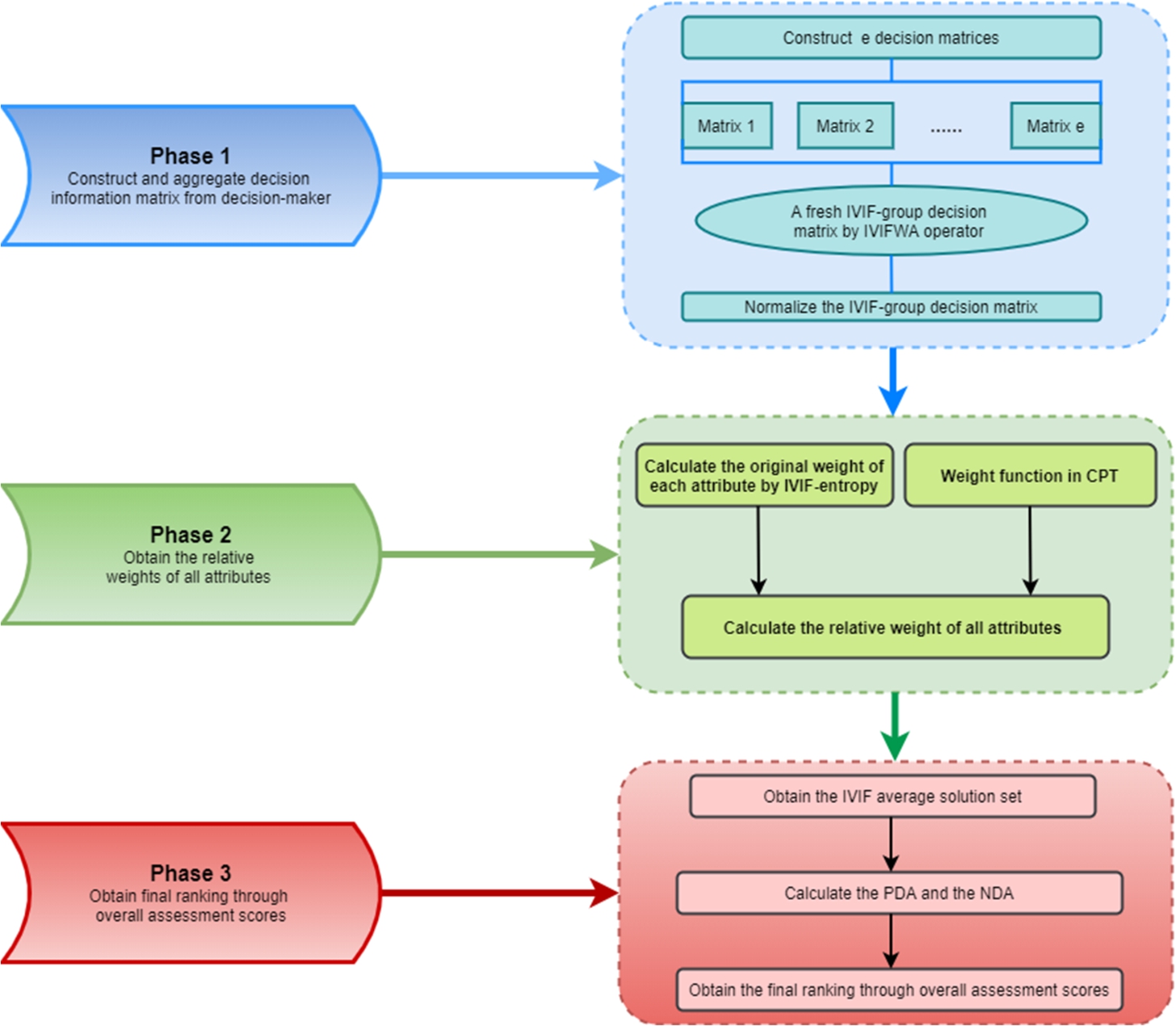
Then, the IVIF-CPT-EDAS detailed steps are as follows (Fig. 2):
Step 1. Obtain the IVIF decision matrix ℵ.
Integrate the IVIF decision matrix
(20)
Step 2. Calculate the normalized IVIF decision matrix
Transform the IVIF decision matrix
(21)
Step 3. Determine the original attribute weight
The specific steps of IVIF-entropy method are shown as follows:
(1) Determine the IVIF negative ideal point (IVIF-NIP):
(22)
(2) Calculate the hybrid distance matrix
(23)
(3) The normalized distance matrix
(24)
(4) Calculate the entropy degree
(25)
(5) Figure out the original attribute weight
(26)
(27)
Step 5. Calculate the relative attribute weight
(28)
Step 6. Calculate the
(29)
(30)
Step 7. Calculate the weighted positive and negative distance (
(31)
(32)
Step 8. The normalized weighted positive and negative distance (
(33)
(34)
Step 9. The overall assessment score
(35)
Step 10. Rank the alternatives by descending order of the overall assessment scores
4An Illustrative Example and Parameter Analysis
4.1Background Description
Development is a timeless topic. However, due to the limitations and irreversibility of resources, it has become a new demand to reduce pollution, save resources, and take the path of sustainable development by developing a green economy. From an investment perspective, GTVC, as one of the five key green investment areas, has a broad space to promote the development of the circular economy, such as comprehensive utilization of resource technology, environmental protection technology, ecological agriculture technology, comprehensive utilization of resource technology, new energy technology, etc. At the same time, evaluating investment projects that can yield significant benefits scientifically and quickly is particularly important for a decision-maker. Therefore, this paper takes the GTVC project selection as an example to verify the effectiveness and applicability of the enhanced EDAS method.
4.2Decision Process
We invite five experts
Here, we will refer to the IVIF linguistic evaluation scale proposed by Peng and Luo (2021) to collect expert evaluation information. The IVIF linguistic evaluation scale table used in this article has a total of 10 evaluation scales, and corresponding IVIFNs are used to quantify the evaluation values of the proposed investment project, in order to achieve accurate DM results. Then the linguistic assessment matrices which are provided in Tables 4 reveal the five DEs’ evaluation results about six attributes.
Table 3
IVIF linguistic evaluation scale.
| Linguistic scale | IVIFN |
| Extremely terrible (ET) | |
| Very terrible (VT) | |
| Terrible (T) | |
| Medium terrible (MT) | |
| Medium (M) | |
| Medium good (MG) | |
| Good (G) | |
| Very good (VG) | |
| Extremely good (EG) | |
| Perfectly good (PG) |
Table 4
The linguistic assessment matrices by five experts.
| DEs | Alternatives | Attributes | |||||
| MG | G | M | G | MG | MG | ||
| VG | M | EG | M | EG | G | ||
| MG | VG | M | MG | G | M | ||
| M | G | MT | M | MG | T | ||
| G | VT | M | M | G | MG | ||
| G | MG | MG | G | M | MG | ||
| EG | MT | EG | M | EG | G | ||
| G | VG | M | M | MG | MT | ||
| MT | G | M | M | G | T | ||
| MG | MT | MT | MT | MG | M | ||
| MG | G | G | MG | G | M | ||
| EG | M | VG | G | EG | G | ||
| MG | G | MG | MG | M | MT | ||
| M | G | M | MG | G | MT | ||
| G | M | VT | M | MG | MG | ||
| G | G | M | G | G | MG | ||
| EG | M | EG | M | VG | VG | ||
| M | EG | MG | MG | MG | M | ||
| MT | G | MG | M | G | MT | ||
| G | MT | MT | M | MG | M | ||
| VG | MG | G | G | MG | G | ||
| EG | MT | EG | MG | VG | VG | ||
| MG | VG | G | MG | G | M | ||
| M | G | MG | M | VG | MT | ||
| VG | M | MT | M | M | MG | ||
Next, the IVIF-CPT-EDAS technique is developed for selecting the best GTVC project.
Step 1. Experts utilize IVIF to provide their own evaluation information, and convert the aforementioned five semantic evaluation matrices into their respective fuzzy decision matrices, refer to Table 3, then aggregate the IVIF decision matrices into a single IVIF group decision matrix using Eq. (20).
Step 2. Since there are mainly two types of attributes, namely benefit and cost, the Eq. (21) can be used to obtain the normalized IVIF decision matrix
Step 3. Determine the original relative attribute weight
Table 5
The normalized IVIF decision matrix
(1) Using the decision information in
(2) Calculate the distance between each alternative solution and IVIF-NIS by employing Eq. (23), then retrieve the hybrid distance matrix
(3) Figure out the entropy degree
(4) Compute the original weight
Table 6
IVIF-NIS
| IVIF-NIP | |||
| IVIF-NIP | |||
Table 7
The normalized hybrid distance matrix
| Hybris distance | ||||||
| 0.209 | 0.138 | 0.217 | 0.000 | 0.022 | 0.260 | |
| 0.364 | 0.306 | 0.466 | 0.182 | 0.605 | 0.393 | |
| 0.131 | 0.000 | 0.193 | 0.176 | 0.144 | 0.122 | |
| 0.000 | 0.120 | 0.124 | 0.337 | 0.229 | 0.000 | |
| 0.296 | 0.436 | 0.000 | 0.354 | 0.000 | 0.225 |
Table 8
The entropy
| 0.821 | 0.778 | 0.785 | 0.839 | 0.625 | 0.814 | |
| 0.179 | 0.222 | 0.215 | 0.161 | 0.375 | 0.186 |
Step 4. Determine the average solution
Table 9
The original attribute weight
| Original attribute weight | ||||||
| 0.134 | 0.166 | 0.160 | 0.121 | 0.280 | 0.139 |
Step 5. Adjusting attribute weights can be achieved by CPT, which involves calculating the relative attribute weights matrix
Step 6. Calculate the distance between each evaluation and
Table 10
The average solution
| Average solution | |||
| Average solution | |||
Table 11
The relative attribute matrix
| 0.202 | 0.230 | 0.226 | 0.190 | 0.314 | 0.219 | |
| 0.215 | 0.238 | 0.234 | 0.190 | 0.308 | 0.219 | |
| 0.202 | 0.230 | 0.226 | 0.190 | 0.314 | 0.207 | |
| 0.202 | 0.230 | 0.226 | 0.204 | 0.314 | 0.207 | |
| 0.215 | 0.238 | 0.226 | 0.204 | 0.314 | 0.219 |
Table 12
The positive distance
| 0.000 | 0.000 | 0.000 | 0.000 | 0.000 | 0.387 | |
| 1.436 | 0.849 | 2.131 | 0.000 | 1.412 | 1.444 | |
| 0.000 | 0.000 | 0.000 | 0.000 | 0.000 | 0.000 | |
| 0.000 | 0.000 | 0.000 | 0.508 | 0.000 | 0.000 | |
| 0.770 | 1.840 | 0.000 | 0.847 | 0.000 | 0.120 |
Steps 7–8. Calculate the weighted positive and negative distance (
Table 13
The negative distance
| 0.740 | 1.824 | 0.775 | 2.566 | 2.068 | 0.000 | |
| 0.000 | 0.000 | 0.000 | 0.418 | 0.000 | 0.000 | |
| 2.464 | 4.251 | 1.333 | 0.491 | 1.023 | 2.170 | |
| 5.126 | 2.151 | 2.799 | 0.000 | 0.384 | 4.124 | |
| 0.000 | 0.000 | 5.184 | 0.000 | 2.240 | 0.000 |
Step 9. Calculate the overall assessment score
Table 14
The normalized weighted distance.
| The normalized weighted distance | |||||
| 0.048 | 1.000 | 0.000 | 0.059 | 0.456 | |
| 0.400 | 0.975 | 0.158 | 0.000 | 0.403 |
Table 15
The overall assessment score
| Overall assessment score | |||||
| 0.224 | 0.987 | 0.079 | 0.029 | 0.429 |
It follows from the above:
Step 10. Based on the final assessment score
4.3Sensitivity Analysis
In this section, we incorporate the effects of CPT on the model and refer to the parameter values given by Tversky and Kahneman (1992): the parameters in weight function
4.3.1The Sensitivity of Parameter α in the Weight Function
We assign the parameter
Table 16
The calculation results with different value of α.
| α | Ranking results | The optimal solution | |||||
| 0.61 | 0.224 | 0.987 | 0.079 | 0.029 | 0.429 | ||
| 0.05 | 0.228 | 0.987 | 0.079 | 0.039 | 0.458 | ||
| 0.15 | 0.227 | 0.987 | 0.079 | 0.037 | 0.453 | ||
| 0.25 | 0.227 | 0.987 | 0.079 | 0.035 | 0.448 | ||
| 0.35 | 0.226 | 0.987 | 0.079 | 0.034 | 0.443 | ||
| 0.45 | 0.225 | 0.987 | 0.079 | 0.032 | 0.438 | ||
| 0.55 | 0.224 | 0.987 | 0.079 | 0.030 | 0.433 | ||
| 0.65 | 0.224 | 0.987 | 0.079 | 0.029 | 0.427 | ||
| 0.75 | 0.223 | 0.987 | 0.079 | 0.027 | 0.422 | ||
| 0.85 | 0.222 | 0.987 | 0.079 | 0.026 | 0.417 | ||
| 0.95 | 0.222 | 0.987 | 0.079 | 0.025 | 0.411 |
According to Table 16, different parameters have little influence on the score results of the IVIF-CPT-EDAS model. With the value of parameter α increase, the overall scores of
4.3.2The Sensitivity Analysis of Parameter β in the Weight Function
We assign the parameter
Table 17
The calculation results of different value of parameter β.
| β | Ranking results | The optimal solution | |||||
| 0.69 | 0.224 | 0.987 | 0.079 | 0.029 | 0.429 | ||
| 0.05 | 0.259 | 0.985 | 0.106 | 0.029 | 0.492 | ||
| 0.15 | 0.254 | 0.985 | 0.102 | 0.029 | 0.484 | ||
| 0.25 | 0.251 | 0.986 | 0.098 | 0.029 | 0.475 | ||
| 0.35 | 0.246 | 0.986 | 0.094 | 0.029 | 0.465 | ||
| 0.45 | 0.240 | 0.986 | 0.090 | 0.029 | 0.455 | ||
| 0.55 | 0.238 | 0.987 | 0.086 | 0.029 | 0.445 | ||
| 0.65 | 0.227 | 0.987 | 0.081 | 0.029 | 0.434 | ||
| 0.75 | 0.219 | 0.988 | 0.076 | 0.029 | 0.423 | ||
| 0.85 | 0.211 | 0.988 | 0.071 | 0.029 | 0.411 | ||
| 0.95 | 0.202 | 0.988 | 0.066 | 0.029 | 0.398 |
According to Table 17, different value of parameter β will cause certain fluctuations to the score results of the IVIF-CPT-EDAS model. With the value increase of parameter β, the overall score of
4.3.3The Sensitivity Analysis of Parameter γ in the Value Function
We assign the parameter
Table 18
The calculation results with different value of parameter γ.
| γ | Ranking results | The optimal solution | |||||
| 0.88 | 0.224 | 0.987 | 0.079 | 0.029 | 0.429 | ||
| 0.05 | 0.275 | 0.987 | 0. 079 | 0. 079 | 0.539 | ||
| 0.15 | 0.265 | 0.987 | 0. 079 | 0. 070 | 0.515 | ||
| 0.25 | 0.257 | 0.987 | 0. 079 | 0.062 | 0.495 | ||
| 0.35 | 0.250 | 0.987 | 0. 079 | 0.056 | 0.479 | ||
| 0.45 | 0.244 | 0.987 | 0. 079 | 0.049 | 0.466 | ||
| 0.55 | 0.238 | 0.987 | 0. 079 | 0.044 | 0.455 | ||
| 0.65 | 0.233 | 0.987 | 0. 079 | 0.039 | 0.446 | ||
| 0.75 | 0.229 | 0.987 | 0. 079 | 0.035 | 0.437 | ||
| 0.85 | 0.225 | 0.987 | 0. 079 | 0.031 | 0.431 | ||
| 0.95 | 0.222 | 0.987 | 0. 079 | 0.027 | 0.426 |
According to Table 18, different values of parameter γ have little influence on the score results of IVIF-CPT-EDAS model. With the value increase of parameter γ, the overall scores of
4.3.4The Sensitivity Analysis with Different Value of Parameter δ in the Value Function
We assign the parameter
Table 19
The calculation result with different value of parameter δ.
| δ | Ranking results | The optimal solution | |||||
| 0.88 | 0.224 | 0.987 | 0.079 | 0.029 | 0.429 | ||
| 0.05 | 0.094 | 0.936 | 0. 000 | 0. 094 | 0.515 | ||
| 0.15 | 0.099 | 0.945 | 0. 000 | 0. 083 | 0.498 | ||
| 0.25 | 0.106 | 0.953 | 0. 000 | 0.069 | 0.482 | ||
| 0.35 | 0.114 | 0.960 | 0. 000 | 0.053 | 0.465 | ||
| 0.45 | 0.122 | 0.967 | 0. 000 | 0.034 | 0.448 | ||
| 0.55 | 0.144 | 0.973 | 0. 016 | 0.029 | 0.440 | ||
| 0.65 | 0.169 | 0.978 | 0. 036 | 0.029 | 0.436 | ||
| 0.75 | 0.194 | 0.983 | 0. 055 | 0.029 | 0.433 | ||
| 0.85 | 0.217 | 0.986 | 0. 074 | 0.029 | 0.430 | ||
| 0.95 | 0.240 | 0.989 | 0. 091 | 0.029 | 0.428 |
According to Table 19, different value of parameter δ will cause certain fluctuations of the score results of IVIF-CPT-EDAS model. With the value increase of the parameter δ, the overall score of the alternative
4.3.5The Sensitivity Analysis of Parameter ρ in the Value Function
We assign the parameter
Table 20
The calculation results with different value of parameter ρ.
| ρ | Ranking results | The optimal solution | |||||
| 2.25 | 0.224 | 0.987 | 0.079 | 0.029 | 0.429 | ||
| 1.55 | 0.224 | 0.987 | 0.079 | 0.029 | 0.429 | ||
| 2.55 | 0.224 | 0.987 | 0.079 | 0.029 | 0.429 | ||
| 3.55 | 0.224 | 0.987 | 0.079 | 0.029 | 0.429 | ||
| 4.55 | 0.224 | 0.987 | 0.079 | 0.029 | 0.429 | ||
| 5.55 | 0.224 | 0.987 | 0.079 | 0.029 | 0.429 | ||
| 6.55 | 0.224 | 0.987 | 0.079 | 0.029 | 0.429 | ||
| 7.55 | 0.224 | 0.987 | 0.079 | 0.029 | 0.429 | ||
| 8.55 | 0.224 | 0.987 | 0.079 | 0.029 | 0.429 | ||
| 9.55 | 0.224 | 0.987 | 0.079 | 0.029 | 0.429 | ||
| 10.00 | 0.224 | 0.987 | 0.079 | 0.029 | 0.429 |
According to Table 20, the overall scores and ranking results remain changed with different ρ.
From the simulation analysis of the above five parameters, it can be seen that despite the slight fluctuations in the model calculation and ranking results caused by changing the parameters in the weight and value functions, the optimal and sub-optimal schemes remain unchanged, demonstrating the IVIF-CPT-EDAS model’s robustness and effectiveness.
5Comparative Analysis
5.1Validity Analysis
In this subsection, we continue to explore the effectiveness of the enhanced EDAS approach based on the same original matrices, the expert weighting vector
5.1.1Comparison with IVIFWA Operator (Xu and Chen, 2007)
The original matrices of this article are substituted by Eq. (16), Eq. (36) and Eq. (37) (Hashemi-Tabatabaei et al., 2019). The calculation results are shown in Table 21, and the optimal alternative is
(36)
(37)
Table 21
The calculation results of IVIFWA operator.
| Alternative | IVIFWA operator | Ranking results | ||
| 0.176 | 0.809 | 3 | ||
| 0.588 | 0.863 | 1 | ||
| 0.126 | 0.812 | 4 | ||
| 0.099 | 0.803 | 5 | ||
| 0.240 | 0.816 | 2 |
Table 22
The calculation results of IVIF-TOPSIS.
| Alternative | Ranking results | |||
| 0.129 | 0.061 | 0.320 | 3 | |
| 0.013 | 0.177 | 0.932 | 1 | |
| 0.150 | 0.040 | 0.212 | 5 | |
| 0.145 | 0.045 | 0.238 | 4 | |
| 0.104 | 0.085 | 0.449 | 2 |
5.1.2Comparison with the IVIF-TOPSIS Method (Izadikhah, 2012)
We substitute the initial data of this article by the IVIF-TOPSIS method (Izadikhah, 2012), which sorts each alternative by determining the relative closeness degree between it and the positive ideal solution. All the outcomes are shown in Table 22, and the optimal alternative is
The DM process is as follows:
Step 1. Calculate the weighted decision matrix Ω using the decision matrix ℵ, IVIFN and original attribute weight ϖ.
Step 2. Determine the IVIF-PIS
(38)
(39)
Step 2. Calculate the distance between each possible solution and IVIF-PIS (IVIF-NIS).
(40)
(41)
Step 3. Calculate the relative proximity degree
(42)
5.1.3Comparison with IVIF-Taxonomy (Xiao et al., 2021)
We substitute the initial data of this article by the IVIF-Taxonomy method (Xiao et al., 2021). All the calculation results are shown in Table 23, and the optimal alternative is
Step 1. Obtain the hybrid distance matrix
(43)
Table 23
The calculation results of IVIF-Taxonomy.
| Alternative | Ranking results | |
| 0.617 | 3 | |
| 0.095 | 1 | |
| 0.708 | 4 | |
| 0.741 | 5 | |
| 0.496 | 2 |
Step 2. The alternatives are homogenized using Eq. (44).
(44)
Step 3. Eq. (45) is used to determine the development mode of alternative schemes, and the optimal alternative is selected according to formulas (46) and (47), as shown in Table 23.
(45)
(46)
(47)
5.1.4Comparison with IVIF-TODIM Method (Krohling and Pacheco, 2014)
Table 24
The calculation results of IVIF-TODIM.
| Alternative | Ranking results | |
| 0.180 | 3 | |
| 1.000 | 1 | |
| 0.018 | 4 | |
| 0.000 | 5 | |
| 0.623 | 2 |
The initial data of this article are substituted by the IVIF-TODIM method (Krohling and Pacheco, 2014). All the outcomes are shown in Table 24, and the optimal alternative is
Step 1. Obtain the normalized IVIF decision matrix
(48)
Step 2. Obtain the normalized attribute weight
(49)
Step 3. The dominance degree between each alternative
(50)
(51)
(52)
Step 4. Calculate the overall dominance degree
(53)
5.2Comprehensive Analysis
Table 25
The ranking results of different DM methods.
| Methods | Order | The best choice | The worst choice |
| IVIFWA (Xu and Chen, 2007) | |||
| IVIF-TOPSIS (Izadikhah, 2012) | |||
| IVIF-TOXONOMY (Xiao et al., 2021) | |||
| IVIF-TODIM (Krohling and Pacheco, 2014) | |||
| IVIF-CPT-EDAS |
Fig. 3
The score value of different DM methods.
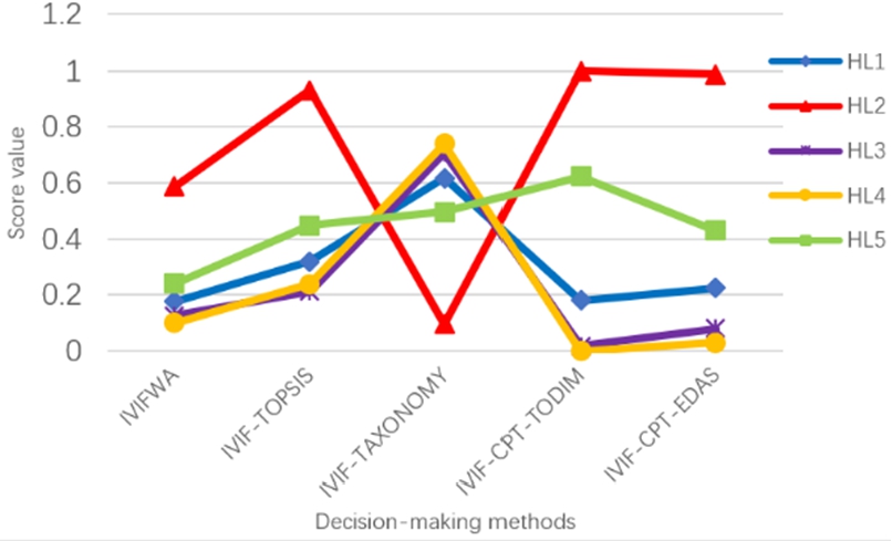
Fig. 4
The ranking results of different DM methods.
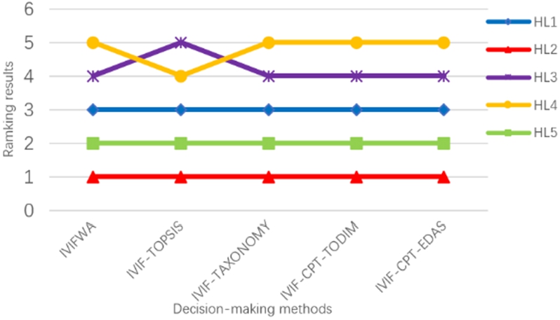
After conducting the validity analysis above and analysing the research results presented in this article, we can conclude that
6Conclusions
In this article, we modified the traditional EDAS method for settling the MAGDM issues better by combining IVIFs. First of all, we briefly review the fundamental definition of IVIFSs, aggregation operator and distance formula. We are aware that the EDAS method is highly effective in resolving DM issues involving contradictory attributes. Therefore, the prominent advantage of introducing the enhanced EDAS technology to IVIFSs in order to address MAGDM problems due to the influence of the actual environment is that it not only lets the average scheme reduce the impact of extreme data, but also takes into account the proximity of the distance between each attribute and the average scheme. Simultaneously, the implementation of the entropy weight method also guarantees the stability of the DM system. Finally, we verified the feasibility of the developed technique by applying the IVIF-CPT-EDAS method to a numerical example of GTVC. Furthermore, sensitivity analysis and several contrast analyses are conducted to validate the rationality and feasibility of MAGDM problems in the practical application process, respectively. Therefore, the main advantages of this paper can be shown as follows: (1) The attribute weights via exploiting information entropy method in IVIFS are constructed. (2) The IVIF-CPT-EDAS approach is designed for addressing MAGDM issues. (3) The presented method of this study not only provides DEs with a broader space for information expression, but also fully considers the psychological characteristics of DEs when facing gains and losses, providing inspiration for subsequent research on DM methods under the framework of bounded rationality.
Nonetheless, the proposed method also has some shortages. On the one hand, the technology developed in this paper solely takes into account the scenario where evaluation information is provided in IVIFs, and real-world evaluation might encounter diverse DM environments. On the other hand, we should thoroughly take into account the genuine psychological alteration trend of decision-makers. Therefore, in future research, we will concentrate on creating novel models and functions for determining attribute weights, enabling them to vary dynamically based on the data. Simultaneously, with the advancement of network technology, numerous DM methods in network form have arisen, including microblog, WeChat, and other online voting forms. In theory, when confronted with such complex DM, we can also extend the findings of this paper to the realm of complex DM that evolves with time.
Compliance with Ethical Standards
Ethical approval
This article does not contain any studies with human participants or animals performed by any of the authors.
Conflict of interest
The authors declare that they have no conflicts of interest.
Data Availability
The data used to support the findings of this study are included within the article.
Acknowledgements
The work was supported by the Sichuan Province Social Development Key R&D Projects under Grant No. 2023YFS0375 and Natural Science Foundation of Sichuan Province under Grant No. 2022NSFSC1821.
References
1 | Agrawal, S., Tyagi, M., Mangla, S.K., Garg, R.K. ((2023) ). Unlocking circular business model avenues to achieve net-zero emissions: a model-driven approach grounded on inter-valued intuitionistic fuzzy sets. Annals of Operations Research. https://doi.org/10.1007/s10479-023-05718-3. |
2 | Amiri, M., Hashemi-Tabatabaei, M., Keshavarz-Ghorabaee, M., Kaklauskas, A., Zavadskas, E.K., Antucheviciene, J. ((2023) ). A fuzzy extension of simplified best-worst method (F-SBWM) and its applications to decision-making problems. Symmetry, 15: (1), 81. |
3 | Atanassov, K.T. ((1986) ). Intuitionistic fuzzy sets. Fuzzy Sets and Systems, 20: , 87–96. |
4 | Atanassov, K.T. ((1994) ). Operators over interval valued intuitionistic fuzzy sets. Fuzzy Sets and Systems, 64: , 159–174. |
5 | Atanassov, K., Gargov, G. ((1989) ). Interval valued intuitionistic fuzzy-sets. Fuzzy Sets and Systems, 31: , 343–349. |
6 | Chen, T.Y. ((2015) ). The inclusion-based TOPSIS method with interval-valued intuitionistic fuzzy sets for multiple criteria group decision making. Applied Soft Computing, 26: , 57–73. |
7 | Chen, T.Y. ((2018) ). An interval-valued Pythagorean fuzzy outranking method with a closeness-based assignment model for multiple criteria decision making. International Journal of Intelligent Systems, 33: , 126–168. |
8 | Dammak, F., Baccour, L., Alimi, A. ((2020) ). A new ranking method for TOPSIS and VIKOR under interval valued intuitionistic fuzzy sets and possibility measures. Journal of Intelligent & Fuzzy Systems, 38: (4), 4459–4469. |
9 | Dhayal, K.S., Giri, A.K., Esposito, L., Agrawal, S. ((2023) ). Mapping the significance of green venture capital for sustainable development: a systematic review and future research agenda. Journal of Cleaner Production, 396: , 136489. |
10 | Dinghong, P., Wenhua, Z. ((2021) ). Sequential group EDAS decision making method for Smart ZeroWaste city selection. Journal of Systems Science and Mathematical Sciences, 41: (3), 688. |
11 | Dong, W., Li, Y., Lv, X., Yu, C. ((2021) ). How does venture capital spur the innovation of environmentally friendly firms? Evidence from China. Energy Economics, 103: , 105582. |
12 | Ecer, F., Böyükaslan, A., Zolfani, S.H. ((2022) ). Evaluation of cryptocurrencies for investment decisions in the era of Industry 4.0: a borda count-based intuitionistic fuzzy set extensions EDAS-MAIRCA-MARCOS multi-criteria methodology. Axioms, 11: (8), 404. |
13 | Fankang, B., Jun, H., Haorun, L., Qiang, F. ((2020) ). Interval-valued intuitionistic fuzzy MADM method based on TOPSIS and grey correlation analysis. Mathematical Biosciences and Engineering, 17: (5), 5584–5603. |
14 | Feng, X., Wei, C., Liu, Q. ((2018) ). EDAS Method for extended hesitant fuzzy linguistic multi-criteria decision making. International Journal of Fuzzy Systems, 20: , 2470–2483. |
15 | Gao, J., Xu, Z.S., Liang, Z.L., Liao, H.C. ((2019) a). Expected consistency-based emergency decision making with incomplete probabilistic linguistic preference relations. Knowledge-Based Systems, 176: , 15–28. |
16 | Gao, J., Xu, Z.S., Ren, P.J., Liao, H.C. ((2019) b). An emergency decision making method based on the multiplicative consistency of probabilistic linguistic preference relations. International Journal of Machine Learning and Cybernetics, 10: , 1613–1629. |
17 | Grzegorzewski, P. ((2004) ). Distances between intuitionistic fuzzy sets and/or interval-valued fuzzy sets based on the Hausdorff metric. Fuzzy Sets and Systems, 148: (2), 319–328. |
18 | Hashemi-Tabatabaei, M., Amiri, M., Ghahremanloo, M., Keshavarz-Ghorabaee, M., Zavadskas, E., Antucheviciene, J. ((2019) ). Hierarchical decision-making using a new mathematical model based on the best-worst method. International Journal of Computers Communications & Control, 14: (6), 710–725. |
19 | Hongjiu, L., Qingyang, L., Yanrong, H. ((2019) ). Evaluating risks of mergers & acquisitions by grey relational analysis based on interval-valued intuitionistic fuzzy information. Mathematical Problems in Engineering, 2019: , 3728029. |
20 | Huang, Y., Lin, R. ((2021) ). An enhancement EDAS method based on Prospect Theory. Technological and Economic Development of Economy, 27: (5), 1019–1038. |
21 | Izadikhah, M. ((2012) ). Group decision making process for supplier selection with TOPSIS method under interval-valued intuitionistic fuzzy numbers. Advances in Fuzzy Systems, 2012: , 407942. |
22 | Jiang, Z.W., Wei, G.W., Chen, X.D. ((2022) ). EDAS method based on cumulative prospect theory for multiple attribute group decision-making under picture fuzzy environment. Journal of Intelligent & Fuzzy Systems, 42: (3), 1723–1735. |
23 | Kahraman, C., Keshavarz Ghorabaee, M., Zavadskas, E.K., Onar, S.C., Yazdani, M., Oztaysi, B. ((2017) ). Intuitionistic fuzzy EDAS method: an application to solid waste disposal site selection. Journal of Environmental Engineering and Landscape Management, 25: (1), 1–12. |
24 | Karasan, A., Kahraman, C. ((2018) ). A novel interval-valued neutrosophic EDAS method: prioritization of the United Nations national sustainable development goals. Soft Computing, 22: , 4891–4906. |
25 | Karunanithi, K., Han, C., Lee, C.-J., Shi, W., Duan, L., Qian, Y. ((2015) ). Identification of a hemodynamic parameter for assessing treatment outcome of EDAS in Moyamoya disease. Journal of Biomechanics, 48: (2), 304–309. |
26 | Keshavarz-Ghorabaee, M. ((2021) ). Assessment of distribution center locations using a multi-expert subjective–objective decision-making approach. Scientific Reports, 11: , 19461. |
27 | Keshavarz-Ghorabaee, M., Zavadskas, E.K., Olfat, L., Turskis, Z. ((2015) ). Multi-criteria inventory classification using a new method of evaluation based on distance from average solution (EDAS). Informatica, 26: (3), 435–451. |
28 | Keshavarz-Ghorabaee, M., Zavadskas, E., Turskis, Z., Antucheviciene, J. ((2016) ). A new combinative distance-based assessment (CODAS) method for multi-criteria decision-making. Economic Computation and Economic Cybernetics Studies and Research / Academy of Economic Studies, 50: , 25–44. |
29 | Keshavarz-Ghorabaee, M., Amiri, M., Zavadskas, E., Turskis, Z., Antucheviciene, J. ((2018) ). Simultaneous evaluation of criteria and alternatives (SECA) for multi-criteria decision-making. Informatica, 29: (2), 265–280. |
30 | Keshavarz-Ghorabaee, M., Amiri, M., Zavadskas, E., Turskis, Z., Antucheviciene, J. ((2021) ). Determination of objective weights using a new method based on the removal effects of criteria (MEREC). Symmetry, 13: (4), 525. |
31 | Keshavarz-Ghorabaee, M., Amiri, M., Zavadskas, E.K., Turskis, Z., Antucheviciene, J. ((2022) ). A fuzzy simultaneous evaluation of criteria and alternatives (F-SECA) for sustainable e-waste scenario management. Sustainability, 14: (16), 10371. |
32 | Krohling, R., Pacheco, A. ((2014) ). Interval-valued intuitionistic fuzzy TODIM. Procedia Computer Science, 31: , 236–244. |
33 | Kumar, K., Chen, S.-M. ((2022) ). Group decision making based on improved linguistic interval-valued Atanassov intuitionistic fuzzy weighted averaging aggregation operator of linguistic interval-valued Atanassov intuitionistic fuzzy numbers. Information Sciences, 607: , 884–900. |
34 | Lee, W.B. ((2009) ). An enhanced multicriteria decision-making method of machine design schemes under interval-valued intuitionistic fuzzy environment. In: 2009 IEEE 10th International Conference on Computer-Aided Industrial Design & Conceptual Design, pp. 721–725. |
35 | Li, S., Wang, B. ((2020) ). Research on evaluating algorithms for the service quality of wireless sensor networks based on interval-valued intuitionistic fuzzy EDAS and CRITIC methods. Mathematical Problems in Engineering, 2020: , 5391940. |
36 | Li, J., Lin, M., Chen, J. ((2012) ). ELECTRE method based on interval-valued intuitionistic fuzzy number. Applied Mechanics and Materials, 220–223: , 2308–2312. |
37 | Li, M., Li, Y., Peng, Q., Wang, J., Yu, C. ((2021) ). Evaluating community question-answering websites using interval-valued intuitionistic fuzzy DANP and TODIM methods. Applied Soft Computing, 99: , 106918. |
38 | Li, Y., Liu, M., Cao, J., Wang, X., Zhang, N. ((2021) ). Multi-attribute group decision-making considering opinion dynamics. Expert Systems with Applications, 184: , 115479. |
39 | Liao, N.N., Gao, H., Lin, R., Wei, G. Chen, X. ((2023) ). An extended EDAS approach based on cumulative prospect theory for multiple attributes group decision making with probabilistic hesitant fuzzy information. Artificial Intelligence Review, 56: , 2971–3003. |
40 | Lin, M., Huang, C., Xu, Z. ((2019) ). TOPSIS method based on correlation coefficient and entropy measure for linguistic Pythagorean fuzzy sets and its application to multiple attribute decision making. Complexity, 2019: , 6967390. |
41 | Lin, M., Wang, H., Xu, Z. ((2020) ). TODIM-based multi-criteria decision-making method with hesitant fuzzy linguistic term sets. Artificial Intelligence Review, 53: , 3647–3671. |
42 | Liu, P.D., You, X.L. ((2019) ). Bidirectional projection measure of linguistic neutrosophic numbers and their application to multi-criteria group decision making. Computers & Industrial Engineering, 128: , 447–457. |
43 | Liu, H.-C., You, J.-X., Duan, C.-Y. ((2019) ). An integrated approach for failure mode and effect analysis under interval-valued intuitionistic fuzzy environment. International Journal of Production Economics, 207: , 163–172. |
44 | Mahmoudi, M., Amoozad Mahdiraji, H., Jafarnejad, A., Safari, H. ((2019) ). Dynamic prioritization of equipment and critical failure modes. Kybernetes, 48: (9), 1913–1941. |
45 | Mishra, A.R., Mardani, A., Rani, P., Zavadskas, E.K. ((2020) ). A novel EDAS approach on intuitionistic fuzzy set for assessment of health-care waste disposal technology using new parametric divergence measures. Journal of Cleaner Production, 272: , 122807. |
46 | Ning, B., Wei, G., Lin, R., Guo, Y. ((2022) ). A novel MADM technique based on extended power generalized Maclaurin symmetric mean operators under probabilistic dual hesitant fuzzy setting and its application to sustainable suppliers selection. Expert Systems with Applications, 204: , 117419. |
47 | Ning, B., Wang, H., Wei, G., Wei, C. ((2023) ). Probabilistic dual hesitant fuzzy MAGDM method based on generalized extended power average operator and its application to online teaching platform supplier selection. Engineering Applications of Artificial Intelligence, 125: , 106667. |
48 | Peng, X., Luo, Z. ((2021) ). Decision-making model for China’s stock market bubble warning: the CoCoSo with picture fuzzy information. Artificial Intelligence Review, 54: (8), 5675–5697. |
49 | Peng, X., Dai, J., Yuan, H. ((2017) ). Interval-valued fuzzy soft decision making methods based on MABAC, similarity measure and EDAS. Fundamenta Informaticae, 152: (4), 373–396. |
50 | Salimian, S., Mousavi, S.M., Antucheviciene, J. ((2022) a). An interval-valued intuitionistic fuzzy model based on extended VIKOR and MARCOS for sustainable supplier selection in organ transplantation networks for healthcare devices. Sustainability, 14: (7), 3795. |
51 | Salimian, S., Mousavi, S.M., Antuchevičienė, J., ((2022) b). Evaluation of infrastructure projects by a decision model based on RPR, MABAC, and WASPAS methods with interval-valued intuitionistic fuzzy sets. International Journal of Strategic Property Management, 26: (2), 106–118. |
52 | Tversky, A., Kahneman, D. ((1992) ). Advances in prospect theory: cumulative representation of uncertainty. Journal of Risk and Uncertainty, 5: , 297–323. |
53 | Wang, C.-Y., Chen, S.-M. ((2017) ). An improved multiattribute decision making method based on new score function of interval-valued intuitionistic fuzzy values and linear programming methodology. Information Sciences, 411: , 176–184. |
54 | Wang, C.-Y., Chen, S.-M. ((2018) ). A new multiple attribute decision making method based on linear programming methodology and novel score function and novel accuracy function of interval-valued intuitionistic fuzzy values. Information Sciences, 438: , 145–155. |
55 | Wei, G., Lan, G. ((2008) ). Grey relational analysis method for interval-valued intuitionistic fuzzy multiple attribute decision making. In: 2008 Fifth International Conference on Fuzzy Systems and Knowledge Discovery, pp. 291–295. |
56 | Wu, L., Gao, H., Wei, C. ((2019) ). VIKOR method for financing risk assessment of rural tourism projects under interval-valued intuitionistic fuzzy environment. Journal of Intelligent & Fuzzy Systems, 37: (2), 2001–2008. |
57 | Xiao, L., Wei, G.W., Guo, Y.F., Chen, X.D. ((2021) ). Taxonomy method for multiple attribute group decision making based on interval-valued intuitionistic fuzzy with entropy. Journal of Intelligent & Fuzzy Systems, 41: , 7031–7045. |
58 | Xu, Z. ((2007) ). Methods for aggregating interval-valued intuitionistic fuzzy information and their application to decision making. Control and Decision, 22: , 215–219. |
59 | Xu, Z.-S., Chen, J. ((2007) ). Approach to group decision making based on interval-valued intuitionistic judgment matrices. Systems Engineering – Theory & Practice, 27: (4), 126–133. |
60 | Yang, S.Y., Feng, D.W., Lu, J.J., Wang, C.C. ((2022) ). The effect of venture capital on green innovation: is environmental regulation an institutional guarantee. Journal of Environmental Management, 318: , 115641. |
61 | Ye, J. ((2017) ). Bidirectional projection method for multiple attribute group decision making with neutrosophic numbers. Neural Computing & Applications, 28: , 1021–1029. |
62 | Ye, D., Liang, D., Li, T., Liang, S. ((2021) ). Multi-classification decision-making method for interval-valued intuitionistic fuzzy three-way decisions and its application in the group decision-making. International Journal of Machine Learning and Cybernetics, 12: , 661–687. |
63 | Yue, Q., Zhang, L. ((2020) ). TOPSIS based two-sided matching under interval-valued intuitionistic fuzzy environment in virtual reality technology transfer. IEEE Access, 8: , 101024–101034. |
64 | Zadeh, L.A. ((1965) ). Fuzzy sets. Information and Control, 8: , 338–356. |
65 | Zeng, S.Z., Cao, C.D., Deng, Y., Shen, X.D. ((2018) ). Pythagorean fuzzy information aggregation based on weighted induced operator and its application to R&D projections selection. Informatica, 29: (3), 567–580. |
66 | Zhang, H., Wang, L. ((2022) ). The service quality evaluation of agricultural E-commerce based on interval-valued intuitionistic fuzzy GRA method. Journal of Mathematics, 2022: , 931136. |
67 | Zhang, Z.-G., Hu, X., Liu, Z.-T., Zhao, L.-T. ((2021) ). Multi-attribute decision making: an innovative method based on the dynamic credibility of experts. Applied Mathematics and Computation, 393: , 125816. |
68 | Zhang, N., Su, W., Zhang, C., Zeng, S. ((2022) ). Evaluation and selection model of community group purchase platform based on WEPLPA-CPT-EDAS method. Computers & Industrial Engineering, 172: , 108573. |
69 | Zhang, H., Wang, H., Wei, G. ((2023) ). Spherical fuzzy TODIM method for MAGDM integrating cumulative prospect theory and CRITIC method and its application to commercial insurance selection. Artificial Intelligence Review, 56: , 10275–10296. |
70 | Zhao, M.W., Wei, G.W., Wei, C., Wu, J., Wei, Y. ((2021) ). Extended CPT-TODIM method for interval-valued intuitionistic fuzzy MAGDM and its application to urban ecological risk assessment. Journal of Intelligent & Fuzzy Systems, 40: (3), 4091–4106. |
71 | Zindani, D., Maity, S.R., Bhowmik, S. ((2021) ). Complex interval-valued intuitionistic fuzzy TODIM approach and its application to group decision making. Journal of Ambient Intelligence and Humanized Computing, 12: (1), 2079–2102. |
72 | Zolfani, S., Torkayesh, A., Ecer, F., Turskis, Z., Šaparauskas, J. ((2021) ). International market selection: a MABA based EDAS analysis framework. Oeconomia Copernicana, 12: (1), 99–124. |
73 | Zulqarnain, R.M., Xin, X.L., Saqlain, M., Khan, W.A. ((2021) ). TOPSIS method based on the correlation coefficient of interval-valued intuitionistic fuzzy soft sets and aggregation operators with their application in decision-making. Journal of Mathematics, 2021: , 6656858. |


