Shadow Minimization Boolean Function Reconstruction

2.1Monotone Boolean Function Recognition

Let Bn={(x1,…,xn)|xi∈{0,1},i=1,…,n} denote the set of vertices of the n-dimensional binary (unit) cube. Let α=(α1,…,αn) and β=(β1,…,βn) be two vertices of Bn. α precedes β (by component-wise order), denoted as α≼β, if and only if αi⩽βi for 1⩽i⩽n. α and β are comparable if α≼β or β≼α, otherwise, they are incomparable. A set of incomparable vertices in Bn is also called a Sperner family. A set {α1,…,αk} of elements of Bn is a growing chain if αi≺αj for 1⩽i<j⩽k. A chain is simple if αi≺αj and there is no αr such that αi≺αr≺αj.

The serial number of the vertex α=(a1,…,an) is the natural number a12n−1+a22n−2+⋯+an20, whose binary representation is a1a2…an.

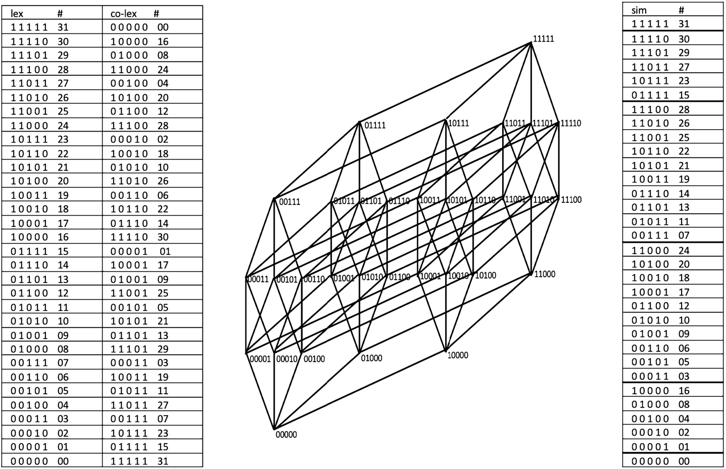
We will also use the lexicographic order of vertices: α precedes β lexicographically (α≼lexβ) if either there exists an integer k, 1⩽k⩽n, such that ak<bk and ai=bi for i<k, or α=β.

In literature there are different, sometimes confusing definitions of lexicographic order (Schröder, 2016). Mathematical definition is set-theoretical that uses the value 1 to code the presence of an element in a subset: x<lexy if min(xΔy)∈x. Appearance of elements in a subset is coded by a binary vector, and vector α precedes vector β when α precedes β alphabetically. Here 1<0. When we apply to combinatorial settings, the hypercube is considered, and lexicographical order of vertices of Bn, defined alphabetically, uses relation 0<1. We will use the standard set-theoretical definition indicated as lex in Fig. 1. revlex is the reverse of this, i.e. (00000,00001,…,11111). colex in set-theoretical settings means: x<co-lexy if max(xΔy)∈y. This is convenient when we add a new dimension to the vectors intending to continue the ordered sequence when the initial segment remains unchanged. But as we see in Fig 1, colex, unlike the lex or revlex, preserves neither the order of numerical values nor the order on the layers of the hypercube graphically, in the Hasse diagram. The sim (simplicial) order lists hypercube vertices layer after the layer (see the next page for the concept of a layer); in each layer, vertices are ordered according to their serial number. We will use the revlex basically, but when there is no confusion we will refer to it simply as lex.

Lexicographic, co-lexicographic and simplicial orders are shown in Fig. 1 on the set of vertices of B5.

Fig. 1

Lexicographic, co-lexicographic and simplicial orders of vertices of B5. The sign # marks the natural order which coincides with the numerical value of binary representation of vertices.

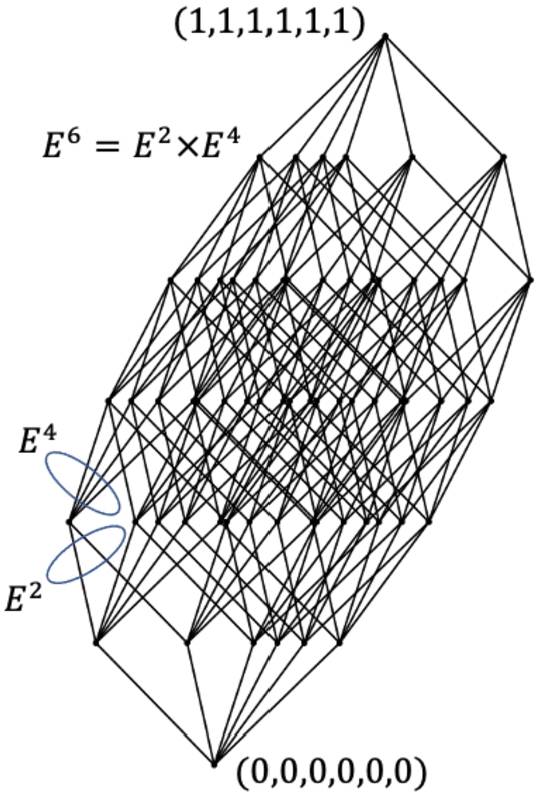
We define also partition/splitting of Bn into two (n−1)-dimensional sub-cubes according to the values of the binary variables; for arbitrary xi:

Figure 2 illustrates the split of the B6 according to two variables.

Fig. 2

Split of the B6 into the B4×B2.

Let Lk={(x1,…,xn)∈Bn|∑i=1nxi=k}. We call Lk the k-th layer of Bn.

The shadow δiM of M⊆Bn is the set of vertices of Li, which are less than some vertex of M.

In case all the vertices of M are from the same layer, e.g. from the k-th layer, the lower (upper, respectively) shadow of M is δk−1M (δk+1M, respectively), i.e. the set of vertices from the (k−1)-th layer, which are less than some vertex of M (from the (k+1)-th layer, which are greater than some vertex of M, respectively).

Boolean function f:Bn→{0,1} is called monotone if for every two vertices α,β∈Bn, if α≺β, then f(α)⩽f(β). Vertices of Bn, where f takes the value “1”, are called units or true points of the function; vertices, where f takes the value “0”, are called zeros or false points of the function. α1 is a lower unit (or minimal true point) of the function if f(α1)=1, and f(α)=0 for every α∈Bn, such that α≺α1. α0 is an upper zero (or maximal false point) of the function if f(α0)=0, and f(α)=1 for every α∈Bn such that α0≺α. minT(f) and maxF(f) denote the sets of minimal true points and maximal false points, respectively. Obviously, minT(f) and maxF(f) are Sperner families in Bn.

Formally, the work with MBFs started in 1897, with the issue of counting their number (Dedekind, 1895). The first algorithmic and complexity-related considerations belong to Korobkov (1965), where, in particular, the valuable concept of resolving subsets was introduced. The final asymptotic estimate about the number of MBFs of n variables was obtained in Korshunov (1981, 2003). The technique on how to introduce and analyse MBFs, is basically presented in Hansel (1966), Korshunov (2003), Lovász (2007).

The Hansel chain structure (Hansel, 1966) was invented in 1966 and played one of the central roles in MBF-related algorithmic techniques.

The next valuable step towards this was taken by Tonoyan (1979), who introduced a set of simple procedures (chain algebra) that serve all the actual queries about Hansel chains, providing a technical solution to all the problems related to algorithms with Hansel chains, without constructing and keeping them in computer memory. A slightly modified and simplified version of Sokolov (1987) is presented using tools such as: enumeration of all chains, and a procedure of finding the i-th vertex of the j-th chain.

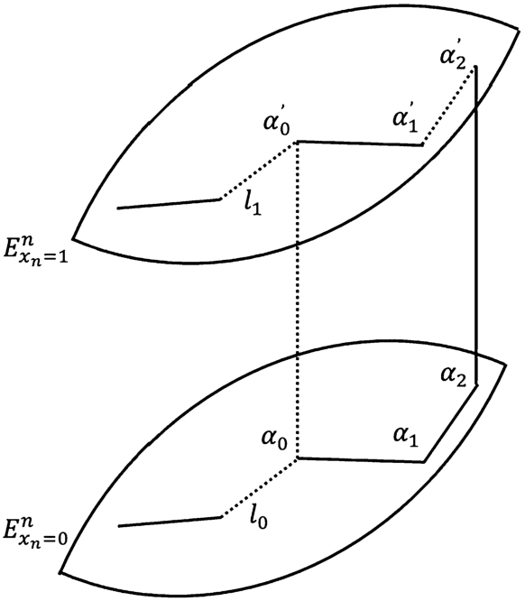
A recurrent step of constructing Hansel chains in Bn is the following (illustrated graphically in Fig. 3). Let l0 be an arbitrary chain in Bxn=0n−1, and let l1, geometrically, be the same chain in Bxn=1n−1. Thorough the chain constructions, all pairs of chains like l0 and l1 are modified according the following rule. Chain l1 is shortened by removing the last edge (α1′,α2′) from it, and chain l0 is updated by adding a new edge (α2,α2′) to it. This construction provides one of the basic properties of Hansel chains in Bn: the relative complement of three consecutive vertices of extended chain l0′ belongs to the shortened chain l1′. Relative complement is a vertex α, that together with the growing chain of tree consecutive vertices α1, α2, α3 composes a subcube of dimension 2.

We aim at extending this picture of chain-split to the lexicographic order of vertices in Bn. At least, we note that the longest Hansel chain corresponds to the chain consisting of the first vertices of layers of Bn under the lexicographic ordering. The mirrored chain of the last vertices under the lexicographic ordering will be considered as well.

Fig. 3

Recurrent step of constructing Hansel chains in Bn.

In the MBF recognition problem using membership queries, the overall goal is to determine an unknown MBF of n variables using as few oracle queries (or tests) as possible. The function can be fully recognized by finding all its upper zeros (and/or lower units) (Korobkov, 1965). The Shannon complexity of finding all upper zeros (lower units) of an arbitrary monotone Boolean function of n variables is Cn⌊n/2⌋+Cn⌊n/2⌋+1 (Hansel, 1966).

Another recognition structure is used in Sokolov (1987) and in its extensions. For even n, Bn is split according to two variables and the recognition starts in the two middle layer sub-cubes of this construction. For odd n, firstly Bn is split according to one variable, then as each sub-cube now has an even size, the procedure for even sizes is applied. This provides optimal recognition of all MBFs in the sense of Shannon complexity. Unfortunately, while simple and attractive, this approach cannot be used as a practical algorithm. Finally, it is worth to mention the work (Gainanov, 1984) that considers not the Shannon complexity, but the individual complexity of MBF given by its resolving set size.

2.2Constraint Monotone Boolean Function Recognition

In general, tasks related to the recognition of MBFs may have different formulations. One objective is to recognize a particular unknown function, knowing that it belongs to the class of MBFs or to one of its subclasses. Another goal is to start with partial knowledge about the unknown function, trying to complete the information. One more case is when the number of queries is restricted by some number k and the goal is to maximize the recognized part of the function (Sahakyan et al., 2022). Similar problems can be formulated for specific classes of Boolean functions. Examples of classes are as follows:

KK-MBF Kruskal-Katona MBFs arise as a result of the shadow minimization theorem (Kruskal, 1963; Katona, 1968, 1987). KK-MBFs are monotone Boolean functions but they also intersect the cube layers along their initial segments of the lexicographic order. The complement of the KK-MBF area in Bn has a similar property; it is related to the initial segments of the reverse-lexicographic order, and they are anti-monotone.

Symmetric MBF This is a trivial class of functions that takes a constant value on the cube layers. Trivial, but these functions are practically important. Examples are majority functions, parity functions, and others (Nosov, 2023).

Threshold MBF Functions are defined by a linear inequality of weighted sums of variables.

Matroid MBF Monotone Boolean function f is called a matroid function if for each α,β∈minT(f) with αi=1, βi=0, there exists a coordinate j with αj=0, βj=1 such that vertex α′, obtained from α by replacing αi with 0 and αj with 1, belongs to minT(f).

The combinatorial complexity of reconstruction in these and other subclasses of MBFs is not well studied. For example, monotone Boolean functions, with zeros and units separated by two middle layers of the cube, are the most difficult functions for query-based reconstruction when only the monotonicity of the function is given. But if it is known that the function belongs to the class of symmetric functions, the reconstruction of this function can be done by n queries. The same function also belongs to the KK-MBF class. Knowing more MBF cases that are practically reconstructible enables system proctoring and application problem solving.

3.1Introduction to KK-MBF Type Functions

The initial formulations of the shadow theorem in Kruskal (1963), Katona (1968, 1987) are given in terms of co-lexicographic order, but this framework was later simplified to the simple lexicographic ordering (Aslanyan, 1979). The basic result was obtained for two neighbour layers of the cube. The name KK now refers to an extension of the basic result of the shadow minimization theorem to many layers of Bn, as well as to results on the existence of Sperner families (Clements, 1973; Daykin et al., 1974). Usually, a KK-MBF function f is given through its characteristics, #minT(f)=⟨pi1,pi2,…,pir⟩, where pij is the number of lower units of f on the ij-th layer. An example is given in Fig. 4.

Fig. 4

KK-MBF function on B5 with p2=2 (vertices 11000 and 10100), p3=1 (vertex 10011), and p4=1 (vertex 01111). Uncoloured vertices show zeros, and the blue vertices – units of the function. Stars indicate the corner points.

3.2Resolving Sets for KK-MBF

First, let us introduce some general concepts from the field of reconstruction of Boolean functions (Korobkov, 1965). Suppose we are given a certain class S of Boolean functions and f∈S.

It follows from the definition that to reconstruct a function it is sufficient to determine its values on some of its resolving sets.

A resolving set G(f,S) is called a deadlock resolving set for (f,S), if no subset of it is resolving for the pair (f,S).

When S is the set of all monotone Boolean functions, then every function f∈S has a unique deadlock resolving set included in all its resolving sets; this is the set G(f)=minT(f)∪maxF(f) (Korobkov, 1965). Thus, for a general MBF, the concept of deadlock resolving set is given by the set of all upper zeros and lower units of the function, which represent two interrelated Sperner systems.

It should be noted that this is not true for other Boolean functions and classes, for example, for the class of symmetric Boolean functions there are no unique deadlock resolving sets.

In this section, we investigate the existence of a deadlock resolving set for KK-MBF functions.

We formulate two simple properties for KK-MBF type functions f and call them horizontal and vertical conditions, denoting them as Cond-h and Cond-v.

Cond-h:

These conditions, applied recursively, define a domain for each vertex α∈f; denote it by d(f,α). Domain is downward when f(α)=0 and upward if f(α)=1. A simple characterization of the domains can be given in terms of natural order of vertices (their serial numbers).

Note that not all vertices of Bn with a higher (smaller) serial number than α, when f(α)=1 (f(α)=0) are part of the d(f,α).

We also define the notion of corner points for KK-MBF type functions.

Let z(f) denote the set of all zero-corner points, and o(f) denote the set of all one-corner points of function f.

Summarizing all the above reasoning, we formulate the following statement.

For a general MBF, it is well-known that |minT(f)∪maxF(f)| can reach the value Cn⌊n/2⌋+Cn⌊n/2⌋+1 and as a consequence, recognition of these functions cannot be done with less complexity. Our first notion about the KK-MBF recognition complexity is an upper bound obtained for the value |z(f)∪o(f)|. Due to the resolving property of the set z(f)∪o(f), the estimate will show the number of required tests for reconstruction of KK-MBF functions.

It is still a question if the value 2(n−1) is reachable. A simple view of exercises in Fig. 4 shows that the real number of corner points will be smaller, but at this point we aim at mentioning the big difference between the recognition complexities of general MBF and the KK-MBF.

Concerning the issue about the size of deadlock resolving sets we may refer to the Theorem 1 of Daykin et al. (1974) and to Clements (1973). Here, parametrized subsets of MBF are considered. Let us suppose that there are given numbers p0,p1,…,pn, denoting the quantities of upper zeros of functions on layers of Bn. Existence theorems of Sperner families, i.e. existence of MBF by the sets {p0,p1,…,pn} are obtained. The first theorem, Daykin et al. (1974), transfers all pi to the layers upper the middle layer. The second theorem (Clements, 1973; Daykin et al., 1974) gives the necessary and sufficient condition of existence in terms of a formula based on Kruskal’s cascade properties (Kruskal, 1963).

Similar theorems could be formulated for KK-MBF, where pis are the numbers of corner points in layers, and then pis can be either 0 or 1. Thus, the formulas would obtain simpler Kruskal’s cascade forms. But in our case, the upper bound 2(n−1) is relatively small and acceptable as a complexity estimation in comparison to Cn⌊n/2⌋+Cn⌊n/2⌋+1. The problem is how to effectively find the mentioned corner points algorithmically.

On the other hand, let us consider a series of KK-MBF functions, which provide a lower bound for |z(f)∪o(f)|.

Define corner points on layers as follows:

On the 1st layer we take two corner points: 1-corner point is the vertex (100…0︷n−1), the smallest vertex of Bx1=1n−1 in lex order; and 0-corner point is (0100…0︷n−2), the smallest vertex of Bx1=0,x2=1n−2 in lex order. These are two neighbour vertices on the 1st layer.

On the 2nd layer we construct two corner points as follows: 1-corner point is (0100…0︷n−31), the smallest vertex of the cube Bx1=0,x2=1,xn=1n−3; 0-corner point is (001100…0︷n−4), the smallest vertex of Bx1=0,x2=0,x3=1,x4=1n−4, all in lex order.

This process is continued until one of the constructed subcubes becomes small and we reach a corner point defined by a 0-size subcube, i.e. a vertex.

Let us explain again the construction. Vertex (100…0︷n−1) is the smallest vertex on layer 1 of Bn. Vertex (0100…0︷n−2) is its left neighbour (see Fig. 4). Vertex (100…0︷n−1) defines all vertices of Bx1=1n−1 as units of the function by Cond-h, and vertex (0100…0︷n−2) defines as zero only the vertex (00…0︷n). Upper area of vertex (0100…0︷n−2) still can be defined arbitrarily – either as a zero or as a unit. But we take the leftmost vertex (0100…0︷n−31) of the layer next to the layer of (0100…0︷n−2) defining its value as unit. The left neighbour’s value we define as zero. This simple construction, repeated as long as possible, gives a series of KK-MBF functions. How many corner points may have these functions?

Starting from the first layer, we reach the last possible corner point on the:

(n/2)-th layer, if n is even – in this case we have 2 corner points on each layer starting from 1 to n/2; and (n+1)/2-th layer, if n is odd – in this case we have 2 corner points on each layer starting from 1 to (n−1)/2, and one corner point on the (n+1)/2-th layer.

In both cases, we get |z(f)∪o(f)|=n; and thus,

3.3Identification of KK-MBF Type Functions: Main Procedures

Hansel chain based MBF recognition methods are global tools and can be applied to recognize any class of monotone Boolean functions, including KK-MBF. However, we aim to exploit specific properties of this class of functions to achieve more efficient recognition. To go beyond the chain-based analysis, in this section we consider the recognition of KK-MBF functions at the level of analysis of particular layers of Bn.

A useful step and exercise in recognitions is to determine the first and last nontrivial layers (trivial layers are those with all-zeros or with all units of the function). This can be done considering the following two chains of length n: L1 that is the chain consisting of all first, and L2 that is the chain consisting of all last elements of the lexicographic order of layers. L1 is the longest Hansel chain in the chain split, see Fig. 3. Applying bisections on chains L1 and L2, we can find two neighbouring layers (k1, k1+1) and (k2, k2+1) and vertices on chains L1 and L2, respectively, where the function’s value changes from 0 to 1. This means that the layers from k2+1 to n, and from 0 to k1 are trivial, they accept values 0 and 1, correspondingly. Indeed, when first vertex of layer k1 accepts 0, then the whole layer accepts 0. The layer k1 and below is filled by values 0 (the trivial 0 layers), but in layer k1+1 there exists at least one vertex with value 1 so that trivial layers interrupt here. Similar explanation is valid concerning the chain L2. The bisection procedure of each chain requires only log2(n) queries to the oracle.

On the other hand, if the vertices on each layer of Bn are ordered lexicographically, we can apply layer by layer bisections and find a corner vertex candidate αk on the k-th layer with no more than log2(Cnk+1) queries.

In this manner, a KK-MBF type function can be recognized by no more than ∑k=1nlog2(Cnk+1) queries. A very rough estimate of this total value would be O(n2), as the largest layer is the middle k-th layer with k=[n/2], where Cn[n/2]∼2n+12πn with n→∞.

For KK-MBF functions the time complexity of Hansel algorithm remains ∼Cn[n/2] so O(n2) is a valuable reduction of the complexity characteristics. But the techniques of Tonoyan (1979) and Sokolov (1987) for the reduction of memory used in Hansel algorithm can not be applied in the case of our layer bisection approach.

To find a way to reduce the memory complexity we continue to address algorithmic questions on layers from an additional perspective. In order to apply bisections on layers, we need to keep all 2n vertices (ordered lexicographically, layer-by-layer) in computer memory. Otherwise, we need to find a vertex by its number in lexicographic order, or by a distance from a certain vertex (again, in lexicographic order). There are no explicit formulas for this. Thus, both cases will require appropriate time and memory resource.

One way to avoid this situation is using sub-cube structures on layers when partitioning the cube. This is easily applicable to find the 0–1 border on layers, although it will require more than logarithmic queries on layers.

We will use αjk for the j-th element of Lk in the lexicographic order. Then the smallest element of Lk in the lexicographic order is α1k=(11…1︷k00…0︷n−k), and the largest one is the element αCnkk= (00…0︷n−k11…1︷)k.

Let Bx1=1n−1 and Bx1=0n−1 be the partitions of Bn according to x1, and Lk,x1=1 and Lk,x1=0 denote the parts of Lk in Bx1=1n−1 and Bx1=0n−1, respectively. Then α1=(011…1︷k00…0︷n−k−1) is the lexicographically smallest element of Lk,x1=0, and α0=(100…0︷n−k11…1︷k−1) is the lexicographically largest element of Lk,x1=1.

Instead of taking the arithmetical middle vertex of Lk to ask/test the function value, we take either α1 or α0 (for certainty, we will take α1). If f(α1)=1, then f(α)=1 for all α∈Lk,x1=1; therefore, the next vertex that we will take to ask the function value is the largest element of Lk,x1=0,x2=0 (the part of Lk in Bx1=0,x2=0n−2), this is element α2=(0011…1︷k00…0︷n−k−2).

If f(α1)=0, then f(α)=0 for all α∈Lk,x1=0; therefore, the next vertex that we will take is the largest element of Lk,x1=1,x2=0 (the part of Lk in Bx1=1,x2=0n−2), this is the element α2=(1011…1︷k−100…0︷)n−k−1.

In general, in Bx1=σ1,…,xi=σin−i the largest element of k-th layer is

σ1…σi11…1︷x00…0︷y, where x is k minus the number of 1s in σ1…σi, and y is (n−k) minus the number of 0s in σ1…σi.

In this way, after each query, we continue in a smaller sub-cube, and hence, the number of queries in each layer can be at most n−1. For the heaviest layer, for k=n/2, we get the same estimate, but without either keeping all vertices in computer memory or calculating the given j-th vertex in the lexicographic order. Indeed, the number of vertices of middle layer equals Cn[n/2]∼2n+12πn when n→∞. Logarithm of this, the number of steps in dichotomy, is equivalent to n−1, and so the partition by cube structures is simple and effective.

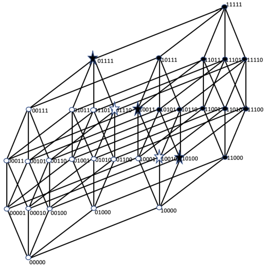
As an example, consider the function given in Fig. 4, and suppose that k=3. Then,

α1=(01110), and since f(01110)=0, the next vertex is

α2=(10110). f(10110)=1, and it follows that the next is

α3=(10011). f(10011)=1.

This way, we found the corner points f(01110)=0 and f(10011)=1 of the third layer.

So far, when recognizing KK-MBF functions layer by layer, we have only used the fact that the function satisfies the condition Cond-h and have not used the monotonicity of the function. Using the monotonicity will narrow the space for taking the next vertex for testing.

Suppose that αk is the smallest vertex of Lk in the lexicographic order with f(αk)=1. Denote by αk+1 the lexicographically smallest upper neighbour of αk in Lk+1. Then, at the next step, we need to consider only those vertices of Lk+1, lexicographically smaller than αk+1.

For the given example in Fig. 4, (10100) is the smallest vertex of L2 in the reverse-lexicographic order, where the function value is 1. Then, we will choose the next vertex in the interval [(00111),(10011)] instead of [(00111),(11100)].

But to calculate the length of the interval [reverse-lexicographically first vertex ofLk+1, αk+1] we need to find the number of αk+1 in lexicographic order. Effective solution of this problem is still open.

Here as well, one can use sub-cube structures, but the benefit is only in the case when f(αk+1)=0.

We conclude the section with the following general note. It addresses an alternative partial order of vertices to the traditional monotony based order, where α≼β if α coordinate-wise precedes β. In terms of KK-MBF, each of the vertices α and β creates 2 domains: upper domains dˆ(f,α) and dˆ(f,β), when f(α)=f(β)=1, and lower domains dˇ(f,α) and dˇ(f,β), when f(α)=f(β)=0. In this case we define the following order: α≼dβ if d(f,α)⊆d(f,β) with f(α)=f(β)=0, and, which is the same, α≼dβ if d(f,α)⊇d(f,β) with f(α)=f(β)=1. Otherwise, vertices α and β are incomparable. We call this construction KK-poset. Sperner type family may be obtained as a simple extension of this concept to the case of KK-poset. Here, similar to general MBFs, each KK-MBF is given by two complementary Sperner families – one is composed by 0-corner points, and the other includes all maximal 1-corner points of the function. We obtain that the KK-MBF reconstruction is similar to the MBF reconstruction, just the basic space and poset is a bit different. The technique developed for the general MBF and the experiences may be used in the problem of reconstruction of KK-MBF functions. We consider this reduction and transfer from MBF to KK-MBF an interesting research topic that is worthy of further investigations.

References

1 | Aslanyan, L.H. ((1979) ). The discrete isoperimetry problem and related extremal problems for discrete spaces. Problemy Kibernetiki, 36: , 85–128. |
2 | Aslanyan, L., Sahakyan, H. ((2009) ). Chain split and computations in practical rule mining. In: Intenational Book Series Information Science and Computing, Book 8, Classification, Forecasting, Data Mining. Institute of Information Theories and Applications, FOI ITHEA, Bulgaria, pp. 132–135. |
3 | Aslanyan, L., Sahakyan, H. ((2017) ). The splitting technique in monotone recognition. Discrete Applied Mathematics, 216: , 502–512. |
4 | Aslanyan, L., Sahakyan, H., Romanov, V., Da Costa, G., Kacimi, R. ((2019) ). Large network target coverage protocols. In: 2019 Computer Science and Information Technologies (CSIT), Yerevan, Armenia, 2019, pp. 57–64. https://doi.org/10.1109/CSITechnol.2019.8895058. |
5 | Aslanyan, L., Gishyan, K., Sahakyan, H. ((2023) a). Target class classification recursion preliminaries. Baltic Journal of Modern Computing, 11: (3), 398–410. |
6 | Aslanyan, L., Katona, G., Sahakyan, H. ((2023) b). Notes on reconstruction of shadow minimization Boolean functions. In: 2023 Computer Science and Information Technologies (CSIT), Yerevan, Armenia, 2023, September 25–30, pp. 119–123. |
7 | Balogh, J., Katona, G.O., Linz, W., Tuza, Z. ((2021) ). The domination number of the graph defined by two levels of the n-cube, II. European Journal of Combinatorics, 91: , 103201. |
8 | Bezrukov, S., Kuzmanovski, N., Lim, J. ((2023) ). Pull-push method: a new approach to edge-isoperimetric problems. Discrete Mathematics, 346: (12), 113632. |
9 | BFA (2023). Ninth Dedekind number discovered: scientists solve long-known problem in mathematics. In: The 8th International Workshop on Boolean Functions and their Applications (BFA), in memory of Kai-Uwe Schmidt, September 3–8, 2023, Voss, Norway. |
10 | Black, H., Chakrabarty, D., Seshadhri, C. (2023). Directed isoperimetric theorems for Boolean functions on the hypergrid and an |
11 | Blum, A. ((2003) ). Learning a function of r relevant variables. In: Learning Theory and Kernel Machines, 16th Annual Conference on Learning Theory and 7th Kernel Workshop, COLT, Kernel 2003, Washington, DC, USA, August 24–27, 2003. Springer, Berlin, Heidelberg, pp. 731–733. |
12 | Boros, E., Hammer, P. ((2002) ). Pseudo-Boolean optimization. Discrete Applied Mathematics, 123: (1–3), 155–225. |
13 | Boros, E., Hammer, P., Ibaraki, T., Kawakami, K. ((1991) ). Identifying 2-monotonic positive Boolean functions in polynomial time. In: ISA’91 Algorithms: 2nd International Symposium on Algorithms Taipei, Republic of China, December 16–18, 1991. Springer, Berlin, Heidelberg, pp. 104–115. |
14 | Braverman, M., Khot, S., Kindler, G., Minzer, D. (2022). Improved monotonicity testers via hypercube embeddings. Preprint: arXiv:2211.09229v1. |
15 | Carlet, C., Joyner, D., Stănică, P., Tang, D. ((2016) ). Cryptographic properties of monotone Boolean functions. Journal of Mathematical Cryptology, 10: (1), 1–14. |
16 | Chao, T.-W., Yu, H.-H.H. (2023). Kruskal–Katona-type problems via entropy method. Preprint: arXiv:2307.15379. |
17 | Clements, G.F. ((1973) ). A minimization problem concerning subsets of a finite set. Discrete Mathematics, 4: (2), 123–128. |
18 | Crawford-Kahrl, P., Cummins, B., Gedeon, T. ((2022) ). Joint realizability of monotone Boolean functions. Theoretical Computer Science, 922: , 447–474. |
19 | Damásdi, G., Gerbner, D., Katona, G.O., Keszegh, B., Lenger, D., Methuku, A., Nagy, D.T., Pálvölgyi, D., Patkós, B., Vizer, M., Wiener, G., ((2021) ). Adaptive majority problems for restricted query graphs and for weighted sets. Discrete Applied Mathematics, 288: , 235–245. |
20 | Daykin, D.E., Godfrey, J., Hilton, A.J.W. ((1974) ). Existence theorems for Sperner families. Journal of Combinatorial Theory, Series A, 17: (2), 245–251. |
21 | Dedekind, R. (1895). Uber die Begründung der Idealtheorie. Gött. Nachr, 106–113. |
22 | Frankl, P., Katona, G.O. ((2021) ). On strengthenings of the intersecting shadow theorem. Journal of Combinatorial Theory, Series A, 184: , 105510. |
23 | Freixas, J. (2022). On the enumeration of some inequivalent monotone Boolean functions. Optimization, https://doi.org/10.1080/02331934.2022.2154126. |
24 | Gainanov, D.N. ((1984) ). On one criterion of the optimality of an algorithm for evaluating monotonic Boolean functions. Zhurnal Vychislitel’noi Matematiki i Matematicheskoi Fiziki, 24: (8), 1250–1257. |
25 | Griggs, J.R., Kalinowski, T., Leck, U., Roberts, I.T., Schmitz, M. ((2023) ). The saturation spectrum for antichains of subsets. Order, 40: , 537–574. https://doi.org/10.1007/s11083-022-09622-6. |
26 | Hansel, G. ((1966) ). Sur le nombre des fonctions Booléennes monotones de n variables. Comptes Rendus de l’Académie des Sciences, 262: (20), 1088–1090. |
27 | Jackson, J.C., Lee, H.K., Servedio, R.A., Wan, A. ((2011) ). Learning random monotone DNF. Discrete Applied Mathematics, 159: (5), 259–271. |
28 | Jung, A. ((2023) ). Shadow ratio of hypergraphs with bounded degree. Graphs and Combinatorics, 39: (3), 40. |
29 | Kabulov, A., Berdimurodov, M. ((2021) ). Parametric algorithm for searching the minimum lower unity of monotone Boolean functions in the process synthesis of control automates. In: 2021 International Conference on Information Science and Communications Technologies (ICISCT), Tashkent, Uzbekistan, 2021, pp. 1–4. https://doi.org/10.1109/ICISCT52966.2021.9670370. |
30 | Katona, G. ((1968) ). A theorem of finite sets. In: Theory of Graphs (Proceedings of the Colloquim held at Tihany). Academic Press, New York. |
31 | Katona, G. (1987). A theorem of finite sets. In: Classic Papers in Combinatorics, pp. 381–401. |
32 | Korobkov, V.K. ((1965) ). On monotone functions of the algebra of logic. Problemy Kibernetiki, 13: , 5–28. |
33 | Korshunov, A.D. ((1981) ). On the number of monotone Boolean menge. Problemy Kibernetiki, 38: , 5–109. |
34 | Korshunov, A.D. ((2003) ). Monotone Boolean functions. Russian Mathematical Surveys, 58: (5), 929. |
35 | Kovalerchuk, B., Delizy, F. ((2005) ). Visual data mining using monotone Boolean functions. In: Visual and Spatial Analysis: Advances in Data Mining, Reasoning, and Problem Solving. Springer, Dordrecht, pp. 387–406. |
36 | Kruskal, J.B. ((1963) ). The number of simplices in a complex. Mathematical Optimization Techniques, 10: , 251–278. |
37 | Kulhandjian, M., Aslanyan, L., Sahakyan, H., Kulhandjian, H., D’Amours, C. ((2019) ). Multidisciplinary discussion on 5G from the viewpoint of algebraic combinatorics. In: 2019 Computer Science and Information Technologies (CSIT), Yerevan, Armenia, 2019, pp. 69–76, https://doi.org/10.1109/CSITechnol.2019.8895166. |
38 | Lange, J., Vasilyan, A. (2023). Agnostic proper learning of monotone functions: beyond the black-box correction barrier. Preprint: arXiv:2304.02700. |
39 | Lovász, L. ((2007) ). Combinatorial Problems and Exercises, 3nd edition. American Mathematical Society. |
40 | Madden, G.N. (2023). Shadows of Colored Complexes and Cycle Decompositions of Equipartite Hypergraphs. PhD thesis, Illinois State University. |
41 | Nosov, M.V. ((2023) ). Estimates of the degrees of separating polynomials for monotone and self-dual functions. Intelligent Systems. Theory and Applications, 27: (2), 79–82. |
42 | O’Donnell, R., Servedio, R. (2005). Learning monotone functions from random examples in polynomial time. CMU School of Computer Science. Citeseer. |
43 | Sahakyan, H. ((2013) ). (0, 1)-matrices with different rows. In: Ninth International Conference on Computer Science and Information Technologies Revised Selected Papers, Yerevan, Armenia, 2013, pp. 1–7. https://doi.org/10.1109/CSITechnol.2013.6710342. |
44 | Sahakyan, H. ((2015) ). On the set of simple hypergraph degree sequences. Applied Mathematical Sciences, 9: (5), 243–253. |
45 | Sahakyan, H. ((2023) ). On nonconvexity of the set of hypergraphic sequences. In: 2023 Computer Science and Information Technologies (CSIT). NAS RA, pp. 47–52. |
46 | Sahakyan, H., Aslanyan, L. ((2017) ). Discrete tomography with distinct rows: relaxation. In: 2017 Computer Science and Information Technologies (CSIT). Yerevan, Armenia, 2017, pp. 117–120. https://doi.org/10.1109/CSITechnol.2017.8312153. |
47 | Sahakyan, H., Aslanyan, L., Katona, G. ((2022) ). Notes on identification of monotone Boolean functions with machine learning methods. In: Proceedings of “Middle-European Conference on Applied Theoretical Computer Science” Conference. Koper, Slovenia, 13–14 October 2022. |
48 | Sales, M., Schülke, B. (2022). A local version of Katona’s intersection theorem. Preprint: arXiv:2206.04278. |
49 | Schröder, B. ((2016) ). Ordered Sets: An Introduction with Connections from Combinatorics to Topology. Birkhäuser. |
50 | Sokolov, N.A. ((1987) ). Optimal reconstruction of monotone Boolean functions. Computational Mathematics and Mathematical Physics, 27: (6), 181–187. |
51 | Tennakoon, R., Suter, D., Zhang, E., Chin, T.-J., Bab-Hadiashar, A. ((2021) ). Consensus maximisation using influences of monotone Boolean functions. In: Proceedings of the IEEE/CVF Conference on Computer Vision and Pattern Recognition, pp. 2866–2875. |
52 | Tonoyan, G.P. ((1979) ). Chain partitioning of n-cube vertices and deciphering of monotone Boolean functions. Journal of Computational Mathematics and Mathematical Physics, 19: (6), 1532–1542. |
53 | Valiant, L.G. ((1984) ). A theory of the learnable. Communications of the ACM, 27: (11), 1134–1142. |
54 | Zhang, E., Suter, D., Tennakoon, R., Chin, T.-J., Bab-Hadiashar, A., Truong, G., Gilani, S.Z. ((2022) ). Maximum consensus by weighted influences of monotone Boolean functions. In: Proceedings of the IEEE/CVF Conference on Computer Vision and Pattern Recognition, New Orleans, LA, USA, 2022, pp. 8964–8972. https://doi.org/10.1109/CVPR52688.2022.00876. |
55 | Zhuravlev, Y.I., Ryazanov, V.V., Aslanyan, L.H., Sahakyan, H.A. ((2019) ). On a classification method for a large number of classes. Pattern Recognition and Image Analysis, 29: , 366–376. |
56 | Zhuravlev, Y.I., Ryazanov, V.V., Ryazanov, V.V., Aslanyan, L.H., Sahakyan, H.A. ((2020) ). Comparison of different dichotomous classification algorithms. Pattern Recognition and Image Analysis, 30: , 303–314. |