
A Parallel Algorithm for Solving a Two-Stage Fixed-Charge Transportation Problem
Abstract
This paper deals with the two-stage transportation problem with fixed charges, denoted by TSTPFC. We propose a fast solving method, designed for parallel environments, that allows solving real-world applications efficiently. The proposed constructive heuristic algorithm is iterative and its primary feature is that the solution search domain is reduced at each iteration. Our achieved computational results were compared with those of the existing solution approaches. We tested the method on two sets of instances available in literature. The outputs prove that we have identified a very competitive approach as compared to the methods than one can find in literature.
1Introduction
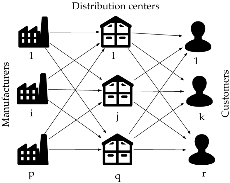
When looking at the definition of supply chains (SCs), we find the commonly accepted variant: they are considered worldwide networks in which the actors are suppliers, manufacturers, distribution centres (DCs), retailers and customers. The typical SC performs several functions; these are: the purchase and processing of raw materials, and their subsequent conversion into intermediary and finished manufactured goods, along with the delivery of the goods to the customers. The major goal of this entire operation is the satisfaction of the customers’ needs and wants.
A particular SC network design problem is the focus of this paper, more specifically, the two-stage transportation problem with fixed charges for opening the distribution centres. This is a modelling problem for a distribution network in a supply chain that is described as two-stage. This two-stage supply chain network design problem includes manufacturers, DCs and customers and its primary feature resides in the fact that for the opening of distribution centres there exist fixed charges added to the variable costs of transportation, that are proportionate to the quantity of goods delivered. The aim of the envisaged optimization problem is to determine which DCs should be opened and to pinpoint and choose the shipping routes, starting from the manufacturers and passing through the picked DCs to reach the customers, and to satisfy all the capacity restrictions at manufacturers and DCs so as to meet the customers’ specific demands, minimizing the total costs of distribution. The problem with this design was considered first by Gen et al. (2006). For a survey on the fixed-charge transportation problem and its variants we refer to Buson et al. (2014), Cosma et al. (2018, 2019, 2020), Calvete et al. (2018), Pirkul and Jayaraman (1998), Pop et al. (2016, 2017), etc.
The variant addressed within the current paper envisages a TSTPFC for opening the DCs, as presented by Gen et al. (2006). The same problem was also considered by Raj and Rajendran (2012). The authors of the two specified papers developed GAs that build, firstly, a distribution tree for the distribution network that links the DCs to customers, and secondly, a distribution tree for the distribution network that links the manufacturers to DCs. In both GAs, the chromosome contains two parts, each encoding one of the distribution trees. Calvete et al. (2016) designed an innovative hybrid genetic algorithm, whose principal characteristic is the employment of a distinct chromosome representation that offers information on the DCs employed within the transportation system. Lately, Cosma et al. (2019) described an effective solution approach that is based on progresively shrinking the solutions search domain. In order to avoid the loss of quality solutions, a mechanism of perturbations was created, which reconsiders the feasible solutions that were discarded, and which might eventually lead to the optimal solution.
The investigated TSTPFC for opening the DCs is an NP-hard optimization problem because it expands the classical fixed charge transportation problem, which is known to be NP-hard, for more information see Guisewite and Pardalos (1990). That is why we describe an efficient parallel heuristic algorithm.
Parallel computing seeks to exploit the availability of several CPU cores which can operate simultaneously. For more information on parallel computing we refer to Trobec et al. (2018).
In this paper, we aim to illustrate an innovative parallel implementation of the Shrinking Domain Search (SDS) algorithm described in Cosma et al. (2019), that is dealing with the TSTPFC for opening the DCs. Our constructive heuristic approach is called Parallel Shrinking Domain Search and its principal features are the reduction of the solutions search domain to a reasonably sized subdomain by taking into account a perturbation mechanism which permits us to reevaluate abandoned feasible solutions whose outcome could be optimal or sub-optimal solutions and its parallel implementation that allows us to solve real-world applications in reasonable computational time. The proposed solution approach was implemented and tested on the existing benchmark instances from the literature.
The paper is organized as follows: in Section 2, we define the investigated TSTPFC for opening the DCs. In Section 3 we describe the novel solution approach for solving the problem, designed for parallel environments. In Section 4 we present implementation details and in Section 5 we describe and discuss the computational experiments and our achieved results. Finally, the conclusions are depicted in Section 6.
2Definition of the Problem
In order to define and model the TSTPFC for opening the DCs we consider a tripartite directed graph
The entire set of vertices V is divided into three mutually exclusive sets corresponding to the set of manufacturers denoted by
In addition, we suppose that:
• Every manufacturer
• Every manufacturer may transport to any of the q DCs at a transportation cost
• Every DC may transport to any of the r customers at a transportation cost
• In order to open any of the DCs we have to pay a given fixed charge, denoted by
In Fig. 1 we present the investigated TSTPFC for opening the DCs.
Fig. 1
Illustration of the considered TSTPFC for opening the DCs.
In order to provide the mathematical formulation of the investigated transportation problem with fixed charges, we consider the following decision variables: the binary variables
Then the TSTPFC for opening the distribution centres can be formulated as the following mixed integer problem, proposed by Raj and Rajendran (2012):
(1)
(2)
(3)
(4)
(5)
(6)
In order to have a nonempty solution set we make the following suppositions:
(7)
(8)
3Description of the Parallel SDS Algorithm
The difficulty of the investigated transportation problem lies in the large number of feasible solutions, from which the optimal option should be chosen. Because each used DC adds a certain cost to the objective function, the fundamental decision of the algorithm is related to the distribution centres that should be used in order to optimize the total distribution costs. Thus, the operations of the algorithm can be separated into the following steps:
S1: Choosing a set of promising distribution centres.
S2: Solving an optimization subproblem in which only the DCs in the chosen set are used.
At the initialization of the algorithm, the number of DCs in the optimal set (DCno) will be estimated based on the minimum capacity of the DCs and the total customer demand. This estimate will be permanently updated throughout the algorithm. If the distribution system has q DCs, then the optimum set search domain has
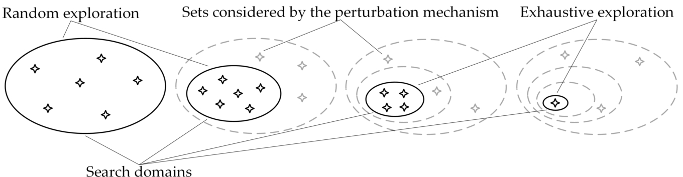
The proposed Parallel Shrinking Domain Search algorithm (PSDS) is an iterative algorithm that applies the following strategy: at each iteration, a fixed number of sets of the search domain will be evaluated, after which the search domain for the next iteration will be reduced. As the search domains narrow down, they will be explored at more detail. In the last iterations, the search domains can be explored exhaustively because they will contain fewer elements than the number settled for evaluation. The algorithm ends when a single set exists in the search domain. In order to avoid losing the optimal solution in the domain search reduction and for DCno estimate adjustment, a perturbation mechanism has been created to reconsider some sets outside the search domain. The search strategy of the PSDS algorithm is shown in Fig. 2.
Fig. 2
The search strategy of the Parallel Shrinking Domain Search algorithm.
The solution-building process is relatively expensive because it requires a large number of operations and the problem is even more complex as the size of the distribution system is larger. The performance of the algorithm has been improved by building solutions in parallel. For this purpose, the Java Fork and Join framework has been used.
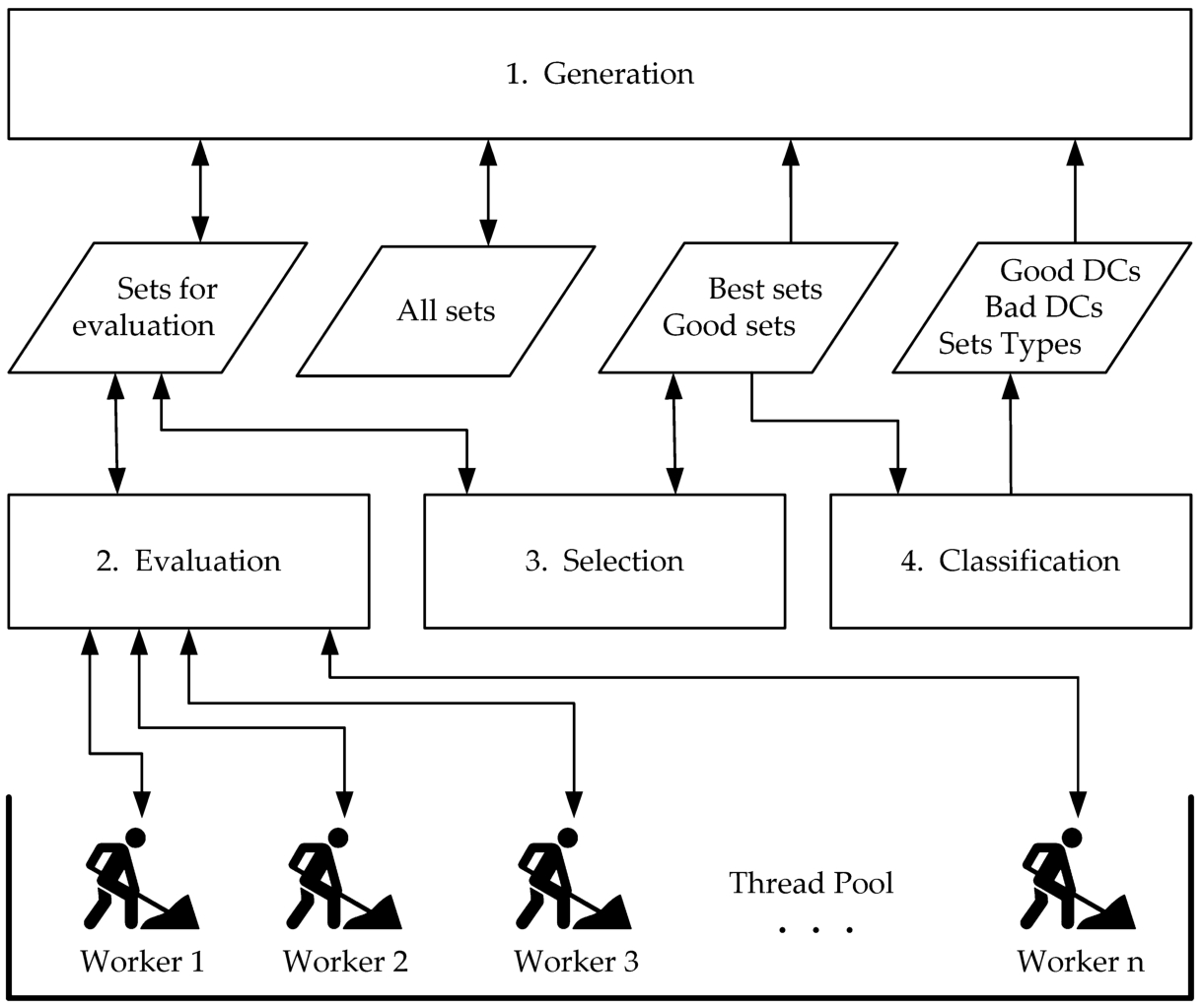
In Fig. 3, we illustrate the operating principle of the proposed PSDS algorithm.
Fig. 3
Our iterative Parallel Shrinking Domain Search algorithm.
The parallel shrinking domain algorithm maintains the following set of lists:
• Good DCs – contains the promising DCs, based on which the sets within the search domain will be generated at every iteration. This list contains the features of surviving sets;
• Bad DCs – a list of disadvantageous DCs that is necessary for the implementation of the perturbation operation, and to correct the DCno estimation;
• Good sets – a list that preserves the best performing sets discovered during the execution of the algorithm. This list has a fixed number of items representing the surviving sets. The sets found at the beginning of this list, contain only good DCs. In the remaining of this document, they will be called Best sets;
• Sets for evaluation – a list of prepared sets for evaluation representing the sets from next generation of sets;
• Sets types – a list that contains a quality estimation of all types of sets found in the Best sets list. This is a list of structures {type, quality};
• All sets – a hash set containing every set created and placed in the Sets for evaluation list during the execution of the algorithm.
At the initialization of the algorithm, the optimal set type (DCno) is estimated and all available DCs are added to the Bad DCs list. Then the Good Sets list, the Sets for evaluation list and the All sets hash set are constructed and a single item of DCno type and
Every iteration of the proposed algorithm executes in sequence the four main blocks presented in Fig. 3: Generation, Evaluation, Selection and Classification. The first block prepares the sets to be evaluated, the second one deals with the evaluation of the sets, and the last two handle the results. From the point of view of complexity, the first and the last two blocks are negligible in relation to the second. The efficiency of the algorithm has been significantly improved by parallel implementation of the processing in the Evaluation block.
The Generation block contains three types of generators for feeding the Sets for evaluation list. All the sets created during the algorithm are kept in a hash set All Sets. Thus, each duplicate can be detected and removed easily. Such a mechanism could be implemented because the total number of sets is relatively small. The optimization process ends after a very small number of iterations. The total number of sets generated during the execution of the algorithm is relatively small. Due to this property, the PSDS algorithm can be applied for solving large instances of the problem.
The first generator type creates a fixed number of sets by picking at random DCs from the Good DCs list. The types of the created sets are retrieved from the Best types list. For each type present in this list, a number of sets proportional to the quality of the type are generated. The quality of the type is determined by the Classification block.
The second generator type creates perturbations by inserting “bad” distribution centres taken from the Bad DCs list in the good sets from the Good sets list. This operation is essential for our optimization process: there could be distribution centres erroneously categorized by the Classification module, because they were found only in sets composed mainly by “bad” distribution centres. Due to the perturbation mechanism, at each iteration these sets get an opportunity to return to the Good DCs list. This mechanism creates a new set for each “bad” distribution centre in the Bad DCs list, by changing one element of a set taken from the Good sets list. The Good sets list is processed in the order given by the cost of the corresponding distribution solutions. This attempts to place each “bad” distribution centre into the best possible set.
Another key operation is the update of the DCno estimation. For this purpose, both larger and smaller sets than those existing in the Best sets list will be created by the third generator type. For creating larger sets, each “bad” distribution centre is added to the best possible set from the Best sets list. The smaller sets are generated by cloning sets from the Best sets list and randomly deleting one of their elements.
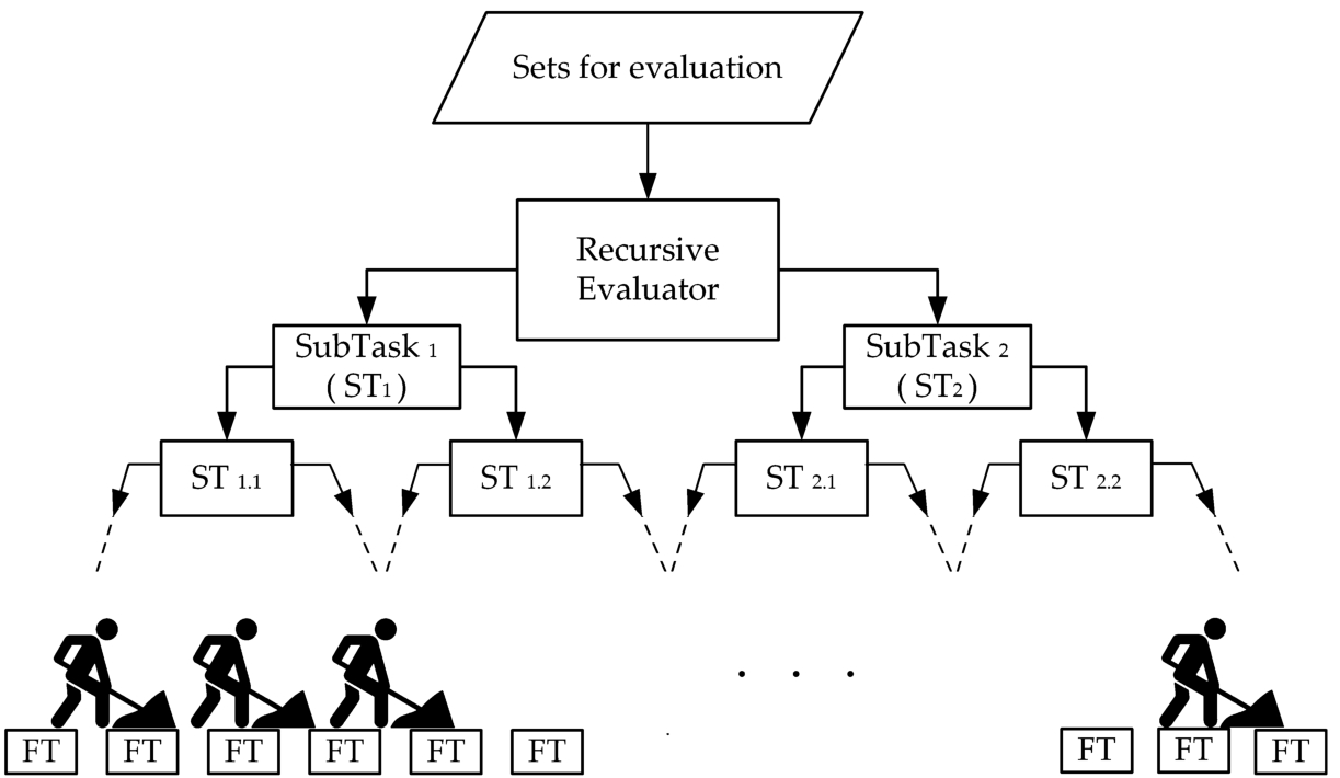
The Evaluation block has the role of evaluating the sets from the Sets for evaluation list. For this purpose, a Recursive Evaluator task is created, which is sent to the Thread Pool for execution.
The operation of this task is shown in Fig. 4. The Recursive Evaluator task divides the Sets for evaluation list into two equal parts, then creates two sub-tasks (ST) to evaluate the two halves. When the number of items a task has to evaluate drops below a certain threshold, a Final Task (FT) is created that will be executed by one of the Worker Threads. For the results presented in this article, a threshold of 10 was used. The algorithm by which each set is evaluated by a FT will be presented at the end of this section.
Fig. 4
The operation of the Recursive Evaluator task.
The Selection and Classification blocks are triggered when all the worker threads have ended. The Selection module takes all the sets in the Sets for evaluation list that are better than the last element in the Good sets list and moves them to that list. Next, the Good sets list is sorted by the set costs and only the best elements are kept, so that its size stays constant. Then the Sets for evaluation list is cleared to make room for the next generation of sets.
The Classification block uses the information in the Good sets list for updating the Good DCs and Bad DCs lists. The Good sets list is traversed based on the cost order. The first distribution centres found in the Good sets elements are added to the Good DCs list, and the remaining ones form the Bad DCs list. The number of sets selected to form the Good sets list decreases each time. Due to this, the PSDS algorithm ends after a small number of iterations.
The Classification block estimates the quality of the set types in the Best sets list and places the result in the Sets types list. The quality of each set type is estimated based on the number of items of that type found in the Best sets list and the positions of those items in the list.
The DC set evaluation operation is presented in Fig. 5.
Fig. 5
The DC set evaluation operation.
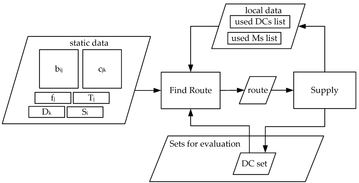
The relatively bulky data structure representing the characteristics of the distribution system (the unit costs
Each solution is constructed in r stages. At each stage the best supply variant for one customer is searched for. Every decision taken in this stage will affect all decisions to be taken in the next stages, as certain transport links might be opened and some of the capacities of manufacturers and distribution centres will be consumed.
Each customer demand is resolved in one or a few stages. At every stage, the cheapest Manufacturer – Dictribution Centre – Customer supply route is sought by the Find Route module, that performs a greedy search. The cost of a route depends on the amount of transported goods, the unit costs of the transport lines and the fixed costs of the transport lines that have not been opened previously. If the found route can not ensure the entire demand of the customer, because of the limited capacities of the distribution centres and manufacturers, then an extra stage is added for the remaining quantity.
The Supply module only uses the two local lists as storage area and updates the total unit costs corresponding to the distribution solution. The last operations of the Supply module is the removal of the unused distribution centres from the evaluated set, and the addition of the remaining distribution centres fixed costs to the final cost of the set.
4Implementation Details
In the description of our algorithm we will use the following abbreviations:
| Zbest | the cost of the best distribution solution; |
| Zworst | the cost of the distribution solution corresponding to the last of the Good sets; |
| Zs | the cost of the distribution solution corresponding to set s; |
| totalQuality | sum of the qualities of all types in the Sets types list; |
| sType | the type of set s; |
| totalSets | the number of sets kept in the Good sets list after each iteration; |
| bestSetsNo | the number of items in the Best sets list; |
| goodPercent | the percentage of the total number of distribution centres that are placed in the Good DCs list; |
| goodDCsNo | the number of items in the Good DCs list; |
| speed | the rate of decreasing the goodPercent; |
| AllDCs | the list with all the distribution centres. |
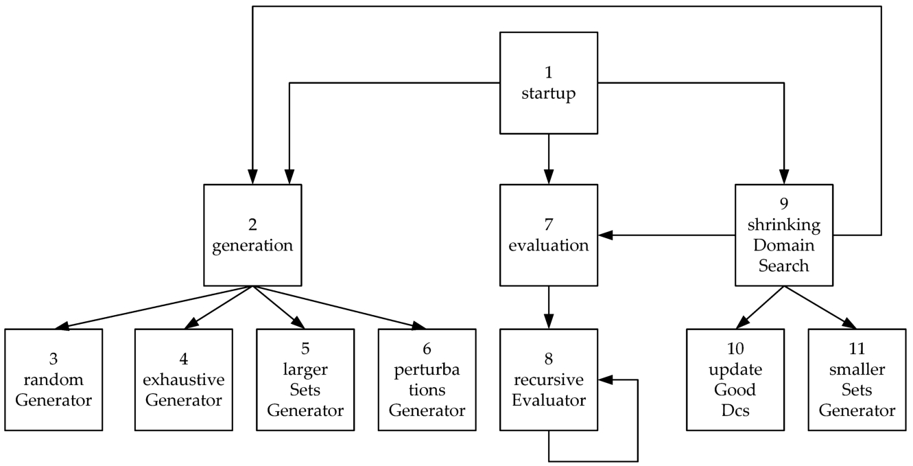
The hierarchy of the procedures that make up the PSDS algorithm is shown in Fig. 6.
Fig. 6
The hierarchy of the PSDS algorithm procedures.
The startup of the algorithm is presented in Algorithm 1. Based on experiments, the following initialization parameters were used:
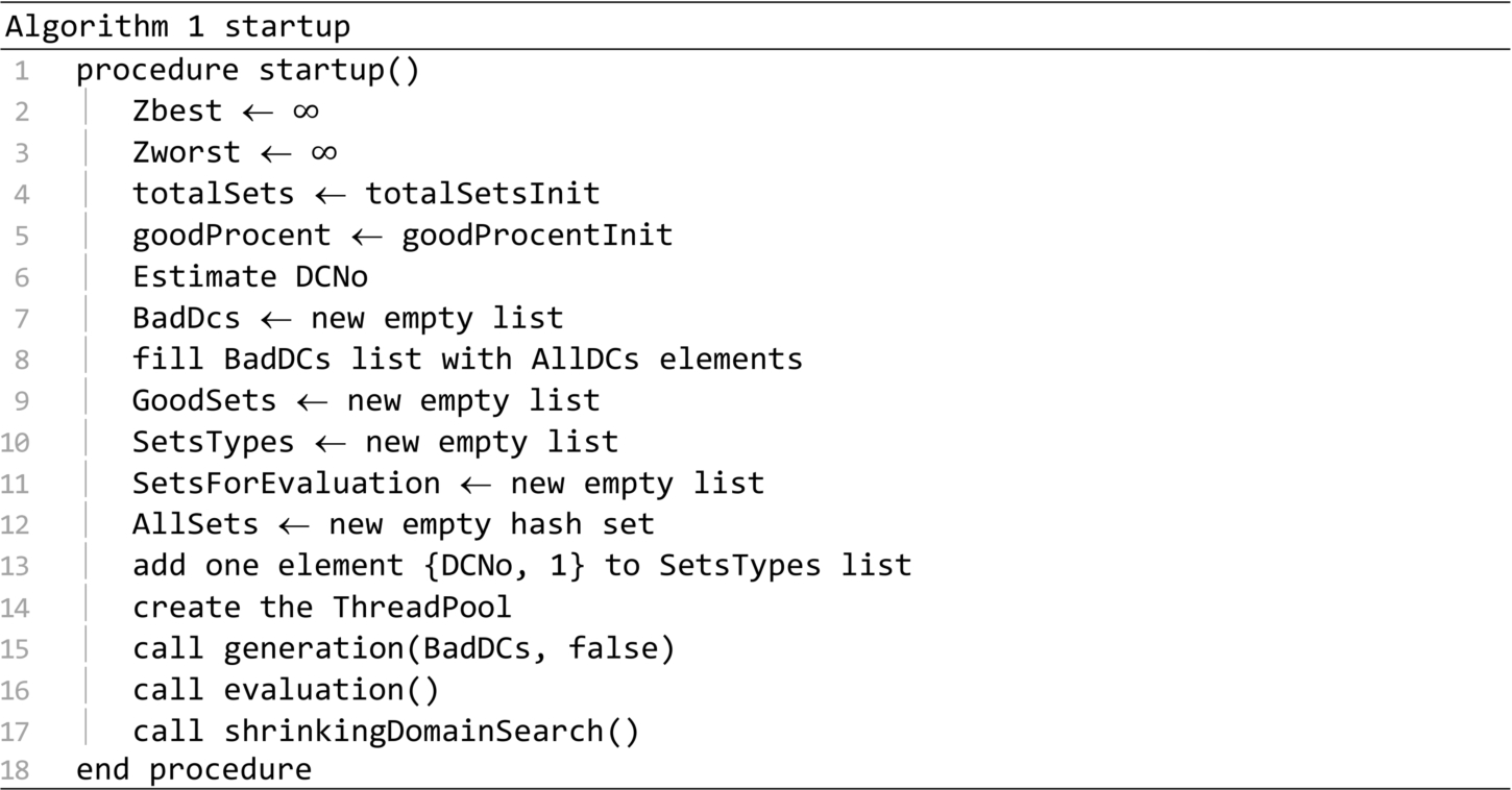
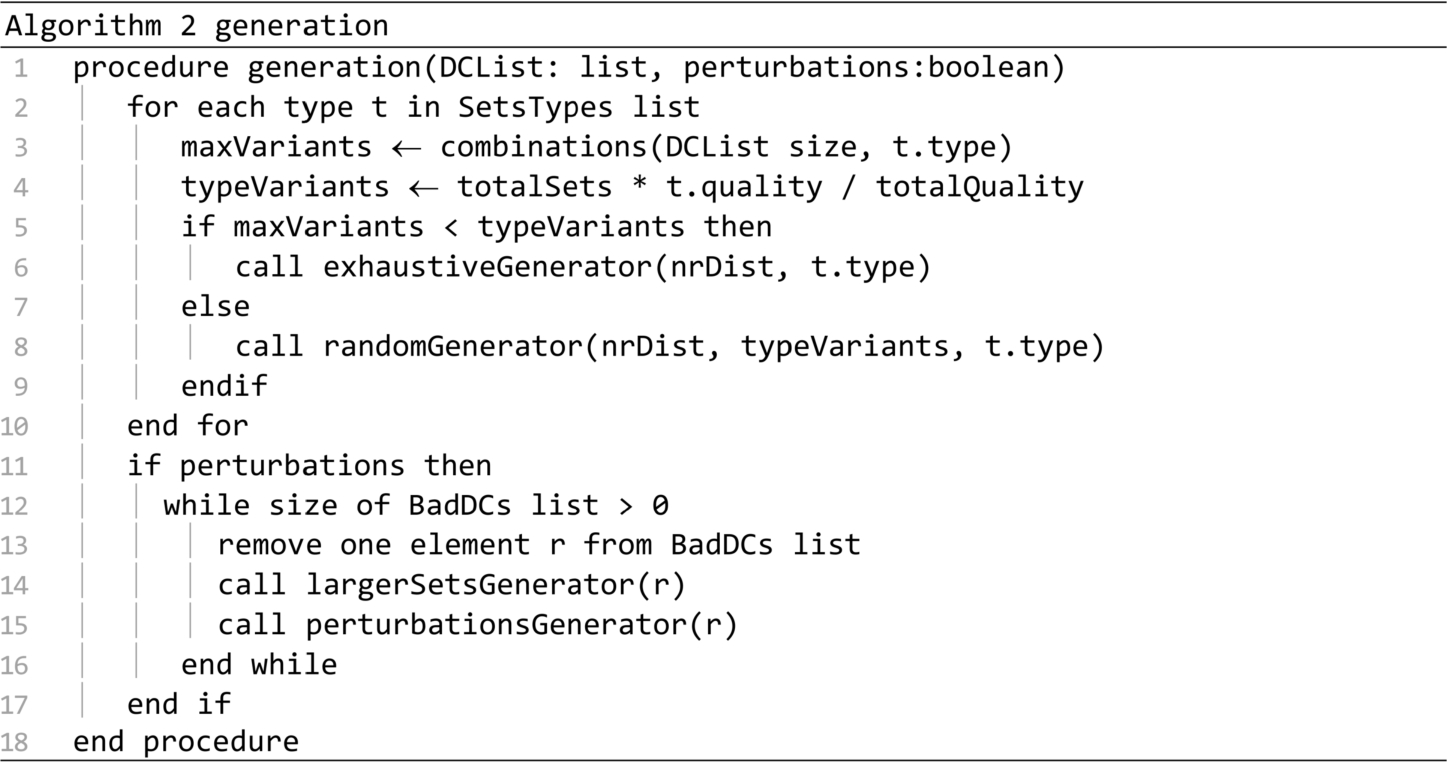
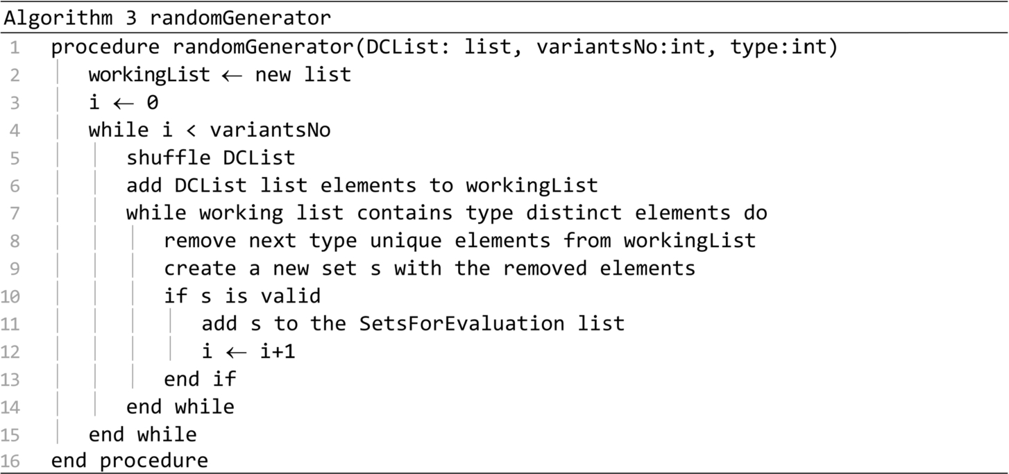
The generation procedure is presented in Algorithm 2. It generates multiple sets based on the distribution centres found in the DCList parameter. This procedure produces perturbations only if the second parameter is true. Petrurbations are almost always generated. The only exception occurs in the case of the call on line 15 of the startup procedure. A number of sets equal to totalSets will be generated at most. For each set type in the SetsTypes list, a number of sets in proportion with the set quality will be generated. If the DCList does not have enough elements for generating the required amount of sets, then the exhaustiveGenerator procedure will be called to generate all the possible sets. Otherwise procedure randomGenerator will be called. If perturbations are required, then the procedures largerSetsGenerator and perturbationsGenerator are called for each distribution center in the BadDCs list.
The randomGenerator procedure presented in Algorithm 3 creates at least variantsNo random sets of certain type with distribution centres taken from the DCList. The new created sets are added to the Sets for evaluation list. The procedure shuffles the distribution centres in a working list and avoids putting a distribution centre multiple times in the same set. Each set is validated on line 10. For a valid set, the sum of the distribution centres capacities must be large enough to satisfy all the customers, and the set has to pass the Duplicates detector.
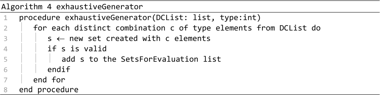
The exhaustiveGenerator procedure is presented in Algorithm 4. It generates all possible sets of certain type with the distribution centres from the DCList. The newly created sets are validated on line 3 and added to the Sets for evaluation list.
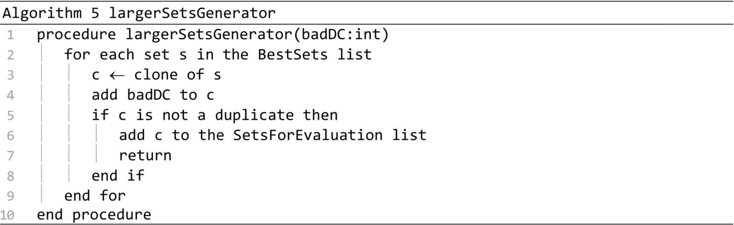
The largerSetsGenerator procedure is presented in Algorithm 5. It searches through the Best sets list to find the best ranked set in which the badDC can be inserted to create a new validated set. The procedure is called in line 14 of the generation procedure, aiming to insert each bad distribution centre in a new valid set.
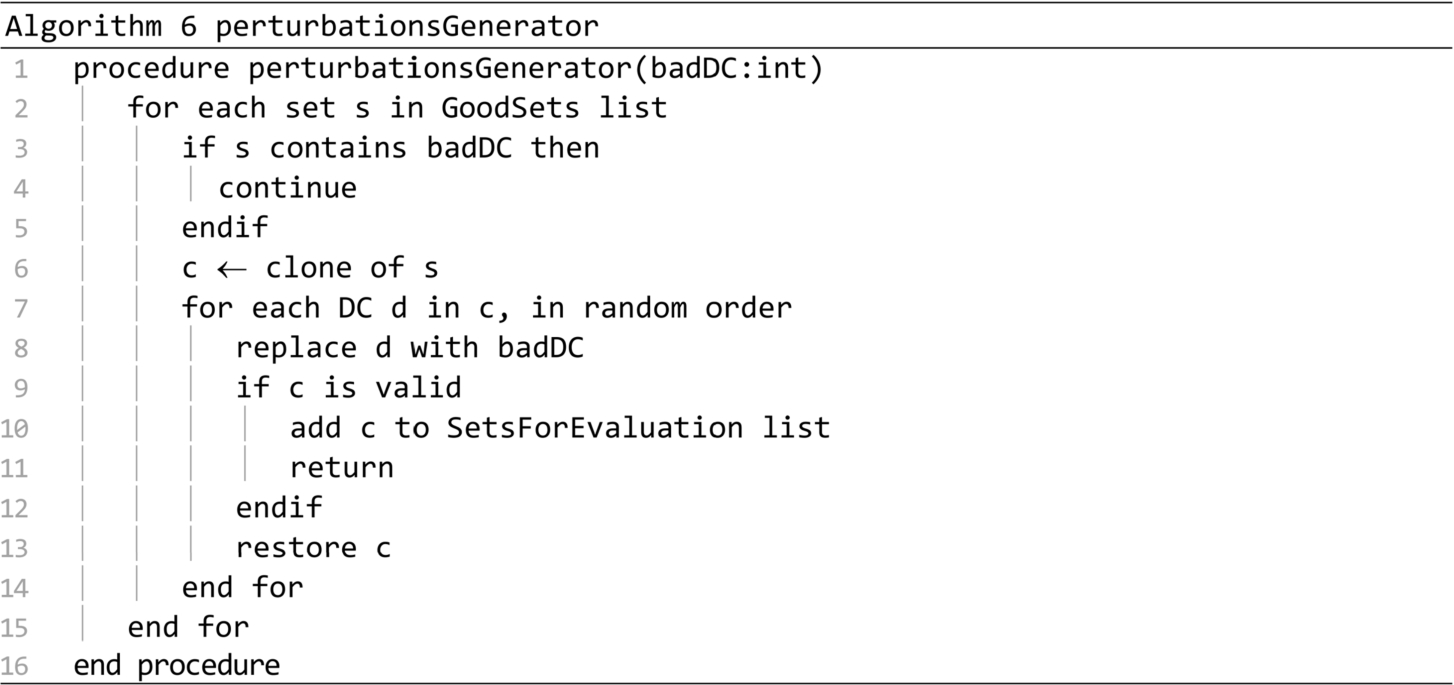
The perturbationsGenerator procedure presented in Algorithm 6 searches in the Good sets list, the first set in which an item can be substituted by the badDC. All the new created sets are added to the Sets for evaluation list. The procedure is called in line 15 of the generation procedure. It tries to insert each “bad” distribution centre in the best possible set.
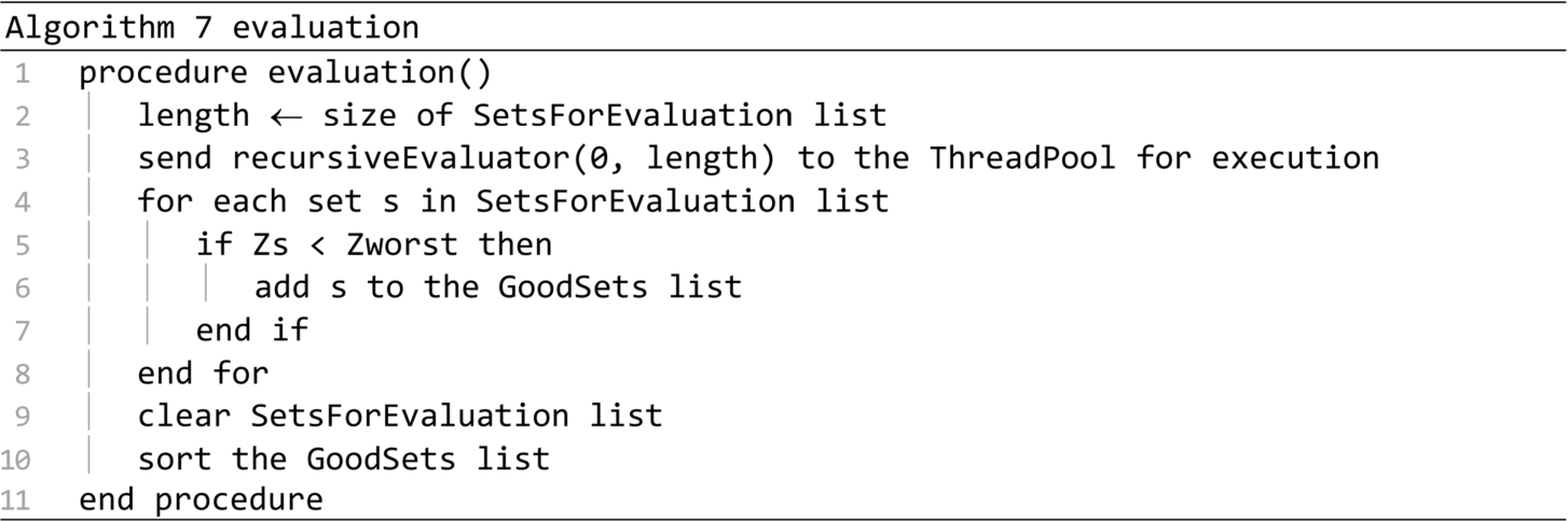
The evaluation procedure is presented in Algorithm 7. It is called in the startup and shrinkingDomainSearch procedures, when the preparation of the Sets for evaluation list is finished. The procedure creates a Recursive evaluator task for all the sets in the Sets for evaluation list, and sends it to the Thread pool for execution. When the evaluation ends, all the sets that are not worse than the ones in the Good sets list are moved to that list. The Sets for evaluation list is cleared, to be prepared for a new iteration, and the Good sets list is sorted according to sets cost.
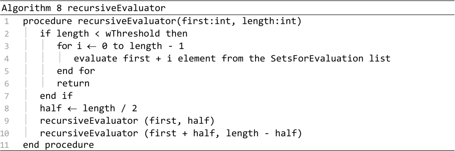
The recursiveEvaluator procedure is presented in Algorithm 8. The first parameter represents the position of the first set from the SetsForEvaluation list to be considered, and the length parameter represents the number of sets to be evaluated, starting from the first. If the value of the length parameter exceeds the value of the threshold wThreshold, then through the calls on lines 9 and 10 two sub-tasks are created, each having to evaluate half of the initial number of sets. When the length parameter falls below wThreshold, the procedure is converted into a Final Task that is retrieved and executed by one of the available Worker Threads in the Thread Pool.
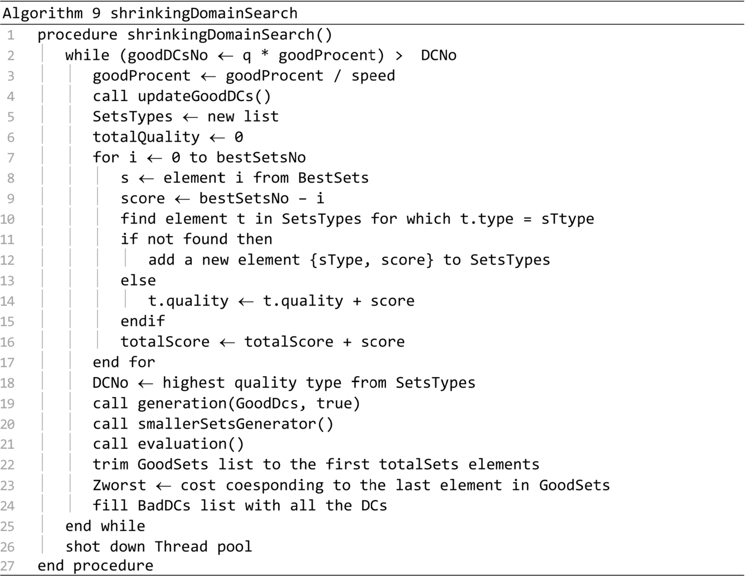
The shrinkingDomainSearch presented in Algorithm 9 is the central procedure of the PSDS algorithm. The search domain is reduced at every iteration of the main loop, by decreasing the goodPercent. Therefore, the goodDCsNo is also reduced. The speed parameter controls the convergence of the algorithm. By increasing the speed parameter, the total number of iterations is reduced. This reduces the total number of operations, the algorithm runs quicker, but the optimal solution might be lost, because the search domains are explored less thoroughly. For the results included in this paper, the speed parameter was fixed to 1.1. The updateGoodDCs procedure call rebuilds the Good DCs and Bad DCs lists, at each iteration. The for loop estimates the quality of all the set types from the Best sets list, considering the number of items of each type, and the positions of those items in the list. These estimations will determine the number of sets that will be generated for each type. The DCNo estimation is updated on line 18. The generators and evaluation procedures are called at the end of the main loop.
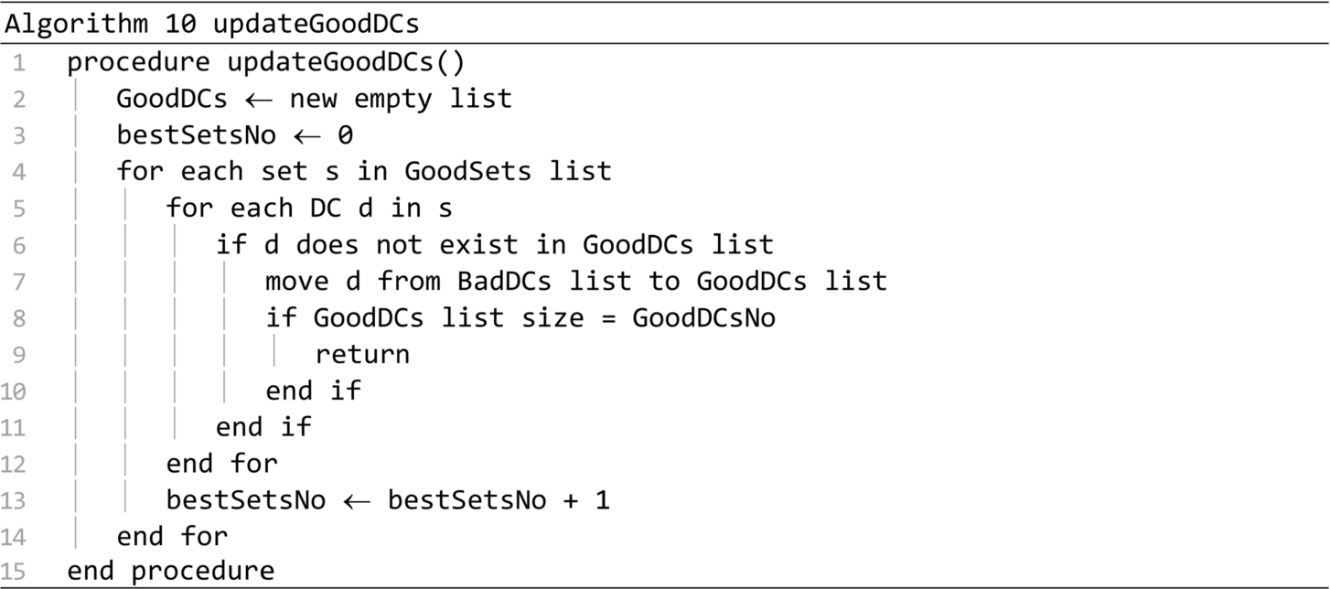
The updateGoodDCs procedure is presented in Algorithm 10. It moves from the Bad DCs list to the Good DCs list a number of distribution centres equal to GoodDCsNo. The distribution centres are taken from the best items of the Good sets list. The bestSetsNo variable is recalculated in the process.
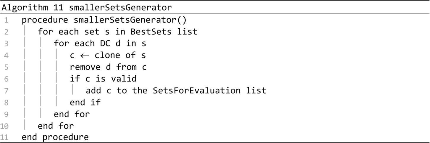
The smallerSetsGenerator procedure presented in Algorithm 11 generates all the possible sets by removing one distribution centre from the items in the Best sets list. Each new created set is validated before being added to the Sets for evaluation list.
The remaining of this section is dedicated to the adjustment of the algorithm’s operating parameters. The charts presented in Figs. 7–12 show the gaps for the average of the best solutions and for the average running times required to find the best solutions, in the cases of four different instances. The selected instances have been run 10 times, using five different values for the following algorithm parameters: speed, goodPercentInit and totalSetsInit.
The gap of the average best solution
(9)
(10)
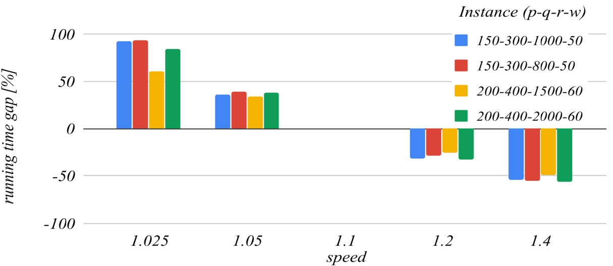
Figures 7 and 8 deal with the speed parameter. The reference value of this parameter that has been set for building the charts is 1.1. For higher values of this parameter, the algorithm ends faster because it performs fewer iterations, but this increases the likelihood of missing the optimal solution, because the search domains are reduced too much with each iteration. For
Fig. 7
The influence of the speed parameter on the best solution found.
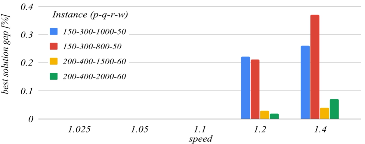
Fig. 8
The influence of the speed parameter on the running time.
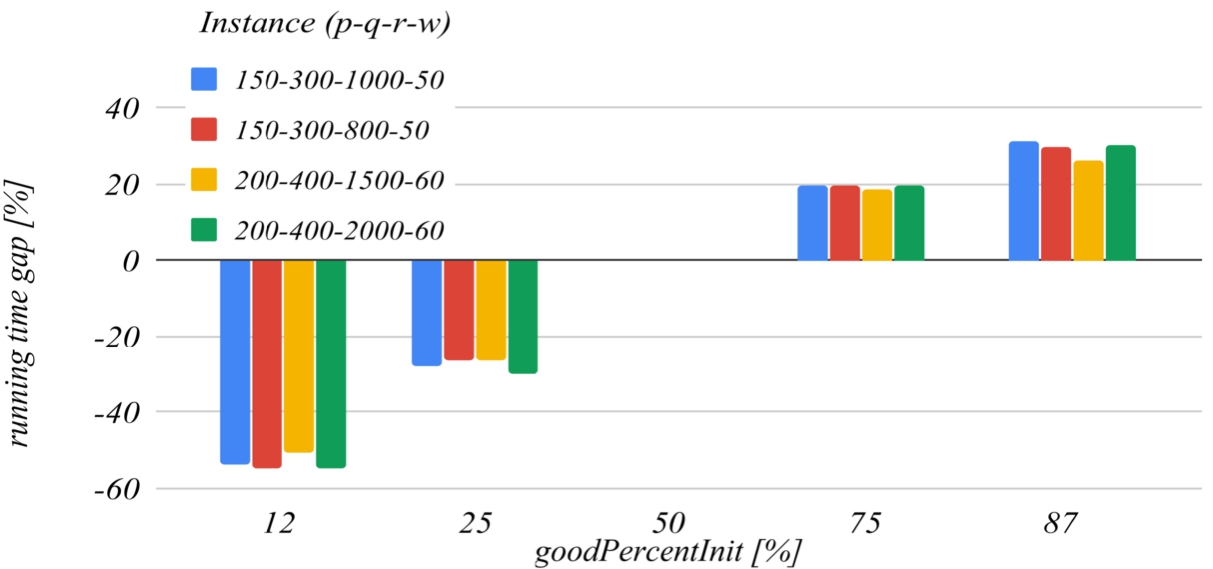
Figures 9 and 10 deal with the goodPercentInit parameter. This parameter determines how much the solution search domain is reduced after the first iteration of the algorithm. The reference value of this parameter that has been set for building the charts is 50. The graph in Fig. 9 shows that the decrease of this parameter below the reference value increases the probability of missing the optimal solution, and the graph in Fig. 10 shows that increasing this parameter over the reference value also unjustifiably increases the running time.
Fig. 9
The influence of the goodPercentInit parameter on the best solution found.
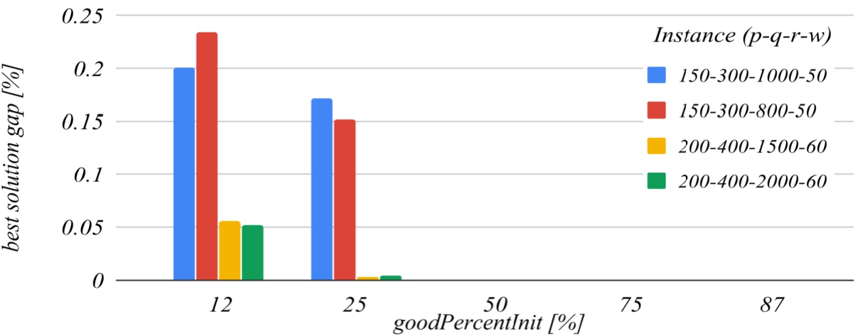
Fig. 10
The influence of the goodPercentInit parameter on the running time.
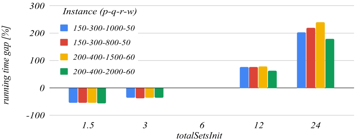
Figures 11 and 12 deal with the totalSetsInit parameter, that is:
Fig. 11
The influence of the totalSetsInit coefficient on the best solution found.
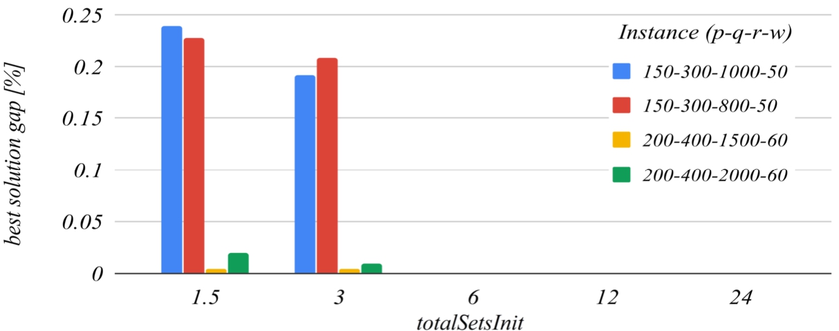
Fig. 12
The influence of the totalSetsInit coefficient on the running time.
5Computational Results
This section is dedicated to the achieved computational results with the aim of assessing the effectiveness of our approaches suggested for solving the TSTPFC for opening the DCs.
The results presented in this section were obtained by running our algorithm for solving the TSTPFC for opening the DCs on a set of 16 test instances of medium sizes, and on a set of 8 instances of larger sizes. Both sets of benchmark instances are known from literature. We refer to Calvete et al. (2016) for more information regarding the characteristics of the first set of instances, and to Cosma et al. (2019) for more information regarding the characteristics of the second set instances.
We implemented our parallel heuristic algorithm for solving the considered transportation problem, in Java language. We have run each of the instances 10 times, as Calvete et al. (2016) did. For our tests, we used two computing systems having the following two significantly different Central Processing Units:
• Intel Core i5-4590 CPU at 3.3 GHz having 4 cores / 4 logical processors;
• Intel Xenon Silver 4114 at 2.2 GHz having 10 cores / 20 logical processors.
For the envisaged test instances, we compared our developed parallel heuristic algorithm with the existing solution approaches with the aim of analysing the performance of our solution. The obtained computational results are presented in Tables 1 and 2.
Table 1
Computational results for the instances introduced by Calvete et al. (2016).
| Instance | LINGO | HEA Calvete et al. | Our solution approach | ||||||
| Zbest | Time | Iteration | Avg. T/It | wt# | |||||
| Best | Avg. | Best | Avg. | ||||||
|
|
|
| 295703 | <0.001 | <0.001 | 1 | 1.00 | <0.001 | 1 |
|
| <0.001 | 0.01 | 1 | 1.00 | 0.01 | 2 | |||
|
| <0.001 | <0.001 | 1 | 1.00 | <0.001 | 4 | |||
|
|
|
| 500583 | <0.001 | <0.001 | 1 | 1.00 | <0.001 | 1 |
|
| <0.001 | <0.001 | 1 | 1.00 | <0.001 | 2 | |||
|
| <0.001 | <0.001 | 1 | 1.00 | <0.001 | 4 | |||
|
|
|
| 803019 | 0.03 | 0.04 | 1 | 1.00 | 0.04 | 1 |
|
| 0.02 | 0.02 | 1 | 1.00 | 0.02 | 2 | |||
|
| 0.02 | 0.02 | 1 | 1.00 | 0.02 | 4 | |||
|
|
|
| 1230358 | 0.05 | 0.06 | 1 | 1.00 | 0.06 | 1 |
|
| 0.02 | 0.03 | 1 | 1.10 | 0.03 | 2 | |||
|
| 0.02 | 0.02 | 1 | 1.00 | 0.02 | 4 | |||
|
|
|
| 1571893 | 0.30 | 0.32 | 1 | 1.20 | 0.28 | 1 |
|
| 0.14 | 0.18 | 1 | 1.30 | 0.14 | 2 | |||
|
| 0.08 | 0.13 | 1 | 1.40 | 0.09 | 4 | |||
|
|
|
| 2521232 | 0.44 | 0.55 | 1 | 1.50 | 0.38 | 1 |
|
| 0.22 | 0.24 | 1 | 1.10 | 0.23 | 2 | |||
|
| 0.14 | 0.17 | 1 | 1.40 | 0.12 | 4 | |||
|
|
|
| 3253335 | 2.31 | 4.49 | 1 | 2.80 | 1.68 | 1 |
|
| 1.20 | 1.95 | 1 | 2.20 | 0.99 | 2 | |||
|
| 0.70 | 1.16 | 1 | 2.10 | 0.60 | 4 | |||
|
|
|
| 4595835 | 3.47 | 3.49 | 1 | 1.00 | 3.49 | 1 |
|
| 1.80 | 1.83 | 1 | 1.00 | 1.83 | 2 | |||
|
| 1.03 | 1.10 | 1 | 1.00 | 1.10 | 4 | |||
|
|
|
| 228306 | <0.001 | 0.02 | 1 | 2.70 | 0.01 | 1 |
|
| <0.001 | 0.01 | 1 | 1.70 | 0.01 | 2 | |||
|
| <0.001 | <0.001 | 1 | 1.70 | <0.001 | 4 | |||
|
|
|
| 348837 | 0.02 | 0.02 | 1 | 2.30 | 0.01 | 1 |
|
| 0.02 | 0.02 | 1 | 2.10 | 0.01 | 2 | |||
|
| <0.001 | 0.01 | 2 | 3.20 | 0.01 | 4 | |||
|
|
|
| 507934 | 0.20 | 0.36 | 2 | 4.30 | 0.09 | 1 |
|
| 0.09 | 0.20 | 2 | 4.90 | 0.04 | 2 | |||
|
| 0.08 | 0.14 | 3 | 5.80 | 0.02 | 4 | |||
|
|
|
| 713610 | 0.31 | 0.61 | 2 | 5.60 | 0.12 | 1 |
|
| 0.20 | 0.32 | 3 | 5.50 | 0.06 | 2 | |||
|
| 0.13 | 0.19 | 2 | 5.20 | 0.04 | 4 | |||
|
|
|
| 985628 | 4.80 | 7.71 | 9 | 13.00 | 0.59 | 1 |
|
| 2.83 | 4.09 | 9 | 13.70 | 0.30 | 2 | |||
|
| 2.28 | 2.84 | 11 | 13.80 | 0.21 | 4 | |||
|
|
|
| 1509476 | 6.75 | 10.91 | 7 | 13.70 | 0.84 | 1 |
|
| 3.28 | 5.96 | 6 | 15.40 | 0.41 | 2 | |||
|
| 3.09 | 4.09 | 10 | 14.70 | 0.29 | 4 | |||
|
|
|
| 1888252 | 72.63 | 92.90 | 14 | 18.30 | 5.08 | 1 |
|
| 32.64 | 45.71 | 12 | 18.10 | 2.53 | 2 | |||
|
| 13.05 | 24.66 | 9 | 18.50 | 1.34 | 4 | |||
|
|
|
| 2669231 | 55.76 | 98.05 | 7 | 13.70 | 7.27 | 1 |
|
| 22.96 | 39.25 | 6 | 11.70 | 3.44 | 2 | |||
|
| 15.91 | 26.32 | 7 | 14.60 | 1.83 | 4 | |||
In Table 1, we describe the results of the computational experiments in the case of the two classes of instances introduced by Calvete et al. (2016). The first column of the table provides the name and the characteristics of the test instance, the next column provides the optimal solution of the problem, denoted by
Table 2
Computational results for the instances introduced by Cosma et al. (2019).
| p |
| Cosma et al. | Our solution approach | ||||||||||
| I | q | IEEE Access | |||||||||||
| # | r | Time [s] | Iteration | CPU | Time [s] | Iteration | Avg. | wt | |||||
| w | Best | Avg | Best | Avg | Best | Avg | Best | Avg | T/It | # | |||
| 1 | 150 300 800 50 | i3 | 47.61 | 112.99 | 8 | 17 | 6.66 | 4 | |||||
| 4c, 4 lp | 41.82 | 191.88 | 3 | 15.85 | 12.21 | 2 | |||||||
| 3.58 GHz | 184.95 | 400.48 | 7 | 16.65 | 24.3 | 1 | |||||||
| 3600012 | 206.79 | 216.52 | 18 | 19.0 | Xeon 10c, 201p 2.2 GHz | 48.99 | 59.15 | 14 | 18 | 3.3 | 20 | ||
| 45.53 | 58.23 | 13 | 17.25 | 3.38 | 16 | ||||||||
| 38.96 | 56.91 | 11 | 16.4 | 3.48 | 12 | ||||||||
| 55.41 | 74.57 | 13 | 18 | 4.18 | 8 | ||||||||
| 99.46 | 129.28 | 12 | 17.00 | 7.67 | 4 | ||||||||
| 467.97 | 492.64 | 17 | 18.75 | 26.42 | 1 | ||||||||
| 2 | 150 300 1000 50 | i3 | 47.42 | 149.35 | 4 | 17.36 | 8.72 | 4 | |||||
| 4c, 4 lp | 139.55 | 260.61 | 10 | 16.97 | 15.37 | 2 | |||||||
| 3.58 GHz | 183.33 | 481.88 | 6 | 16.38 | 29.74 | 1 | |||||||
| 4531394 | 260.37 | 311.11 | 14 | 16.8 | Xeon 10c, 201p 2.2 GHz | 28.28 | 63.83 | 6 | 15.14 | 4.27 | 20 | ||
| 59.09 | 74.92 | 14 | 17.6 | 4.25 | 16 | ||||||||
| 51.8 | 70.8 | 12 | 17.25 | 4.16 | 12 | ||||||||
| 39.83 | 83.4 | 7 | 17.60 | 5.42 | 8 | ||||||||
| 138.01 | 159.82 | 16 | 18.25 | 9.06 | 4 | ||||||||
| 466.01 | 578.98 | 16 | 31.62 | 1 | |||||||||
| 3 | 200 400 1500 60 | i3 | 144.92 | 336.46 | 6 | 15.28 | 22.28 | 4 | |||||
| 4c, 4 lp | 305.63 | 624.35 | 7 | 15.62 | 40.53 | 2 | |||||||
| 3.58 GHz | 635.52 | 1221.32 | 6 | 15.17 | 81.85 | 1 | |||||||
| 6594333 | 468.97 | 721.36 | 8 | 12.8 | Xeon 10c, 201p 2.2 GHz | 99.39 | 176.27 | 9 | 16.92 | 10.49 | 20 | ||
| 112.61 | 166.2 | 10 | 15.4 | 10.86 | 16 | ||||||||
| 140.05 | 192.61 | 12 | 17.1 | 11.29 | 12 | ||||||||
| 90.58 | 199.83 | 6 | 14.6 | 13.89 | 8 | ||||||||
| 175.63 | 338.08 | 6 | 13 | 26.57 | 4 | ||||||||
| 962.04 | 1287.39 | 12 | 15 | 86.09 | 1 | ||||||||
| 4 | 200 400 2000 60 | i3 | 96.54 | 442.01 | 3 | 17.17 | 26.02 | 4 | |||||
| 4c, 4 lp | 344.31 | 848.23 | 6 | 17.58 | 48.53 | 2 | |||||||
| 3.58 GHz | 815.78 | 1681.32 | 8 | 17.32 | 97.66 | 1 | |||||||
| 8828329 | 461.28 | 1020.21 | 7 | 16.2 | Xeon 10c, 201p 2.2 GHz | 144.52 | 215.19 | 11 | 16.92 | 12.79 | 20 | ||
| 147.32 | 224.16 | 10 | 17.2 | 13.13 | 16 | ||||||||
| 144.18 | 230.6 | 9 | 16.9 | 13.8 | 12 | ||||||||
| 51.32 | 265.5 | 2 | 14.8 | 19.27 | 8 | ||||||||
| 404.8 | 506.15 | 13 | 17.25 | 29.46 | 4 | ||||||||
| 1590.44 | 1886.82 | 15 | 17.5 | 108.01 | 1 | ||||||||
| 5 | 250 500 2500 70 | i3 | 321.67 | 1194.81 | 5 | 20.07 | 60.02 | 4 | |||||
| 4c, 4 lp | 1569.33 | 2294.09 | 12 | 20.06 | 114.82 | 2 | |||||||
| 3.58 GHz | 2744.46 | 4276.71 | 11 | 19.38 | 222.91 | 1 | |||||||
| 11055247 | 2709.26 | 2733.78 | 21 | 21.5 | Xeon 10c, 201p 2.2 GHz | 353.18 | 522.15 | 12 | 18.71 | 28.07 | 20 | ||
| 497.03 | 569.26 | 17 | 19.75 | 28.86 | 16 | ||||||||
| 539.16 | 605.85 | 20 | 21.75 | 28.02 | 12 | ||||||||
| 427.66 | 663.61 | 11 | 19.20 | 34.96 | 8 | ||||||||
| 1235.03 | 1368.82 | 20 | 21.00 | 65.19 | 4 | ||||||||
| 4529.15 | 4609.30 | 18 | 19.75 | 235.26 | 1 | ||||||||
| 6 | 250 500 3000 70 | i3 | 658.72 | 1029.29 | 8 | 16.33 | 64.35 | 4 | |||||
| 4c, 4 lp | 733.17 | 2062.34 | 4 | 15.93 | 133.13 | 2 | |||||||
| 3.58 GHz | 1482.97 | 4093.83 | 5 | 15.34 | 271.97 | 1 | |||||||
| 13150463 | 1423.67 | 2275.37 | 8 | 15.0 | Xeon 10c, 201p 2.2G Hz | 443.38 | 588.29 | 13 | 18.08 | 32.54 | 20 | ||
| 264.15 | 452.47 | 7 | 13.29 | 34.5 | 16 | ||||||||
| 448.52 | 586.94 | 13 | 17.83 | 33 | 12 | ||||||||
| 441.11 | 740.31 | 9 | 17.00 | 44.24 | 8 | ||||||||
| 646.10 | 908.02 | 7 | 10.50 | 86.92 | 4 | ||||||||
| 3065.59 | 4712.13 | 10 | 16.25 | 292.96 | 1 | ||||||||
| 7 | 300 600 3500 80 | i3 | 621.07 | 1795.15 | 5 | 17.91 | 101.73 | 4 | |||||
| 4c, 4 lp | 1191.45 | 3653.61 | 5 | 18.57 | 198.91 | 2 | |||||||
| 3.58 GHz | 2869.08 | 7824.73 | 6 | 17.48 | 453.42 | 1 | |||||||
| 15190167 | 1531.77 | 4439.75 | 5 | 15.8 | Xeon 10c, 201 p 2.2 GHz | 414.1 | 894.56 | 7 | 18.33 | 49.7 | 20 | ||
| 510.9 | 947.71 | 9 | 18.4 | 51.9 | 16 | ||||||||
| 732.69 | 1017.76 | 13 | 19.33 | 52.2 | 12 | ||||||||
| 985.16 | 1274.07 | 15 | 19.4 | 65.7 | 8 | ||||||||
| 2284.5 | 2376.73 | 20 | 20.25 | 117 | 4 | ||||||||
| 8520.18 | 8759.55 | 20 | 20.33 | 430.7 | 1 | ||||||||
| 8 | 300 600 4000 80 | i3 | 1381.14 | 2133.52 | 10 | 18.51 | 116.24 | 4 | |||||
| 4c, 4 lp | 2875.94 | 4159.1 | 10 | 19.07 | 220.35 | 2 | |||||||
| 3.58 GHz | 3441.87 | 8269.08 | 8 | 18.35 | 454.77 | 1 | |||||||
| 17266134 | 3046.88 | 5368.18 | 11 | 19.8 | Xeon 10c, 201 p 2.2 GHz | 978.31 | 1116.29 | 18 | 20.25 | 55.25 | 20 | ||
| 784.3 | 1121.98 | 13 | 18.9 | 59.49 | 16 | ||||||||
| 515.16 | 1150.47 | 7 | 19.22 | 60.87 | 12 | ||||||||
| 1265.48 | 1459.72 | 17 | 20 | 73.07 | 8 | ||||||||
| 1540.24 | 2168.33 | 10 | 14.75 | 148 | 4 | ||||||||
| 6721.36 | 8589.16 | 12 | 17 | 512.2 | 1 | ||||||||
The results in Table 1 show that our developed parallel heuristic algorithm delivers the same result as the one provided by Calvete et al. (2016), in all ten runs of computing experiments. These results correspond to the optimal solutions of the problem obtained by LINGO. In terms of efficiency, our parallel heuristic algorithm runs faster than the hybrid evolutionary algorithm proposed by Calvete et al. (2016) when using a single working thread and our calculation runtimes decrease as the number of worker threads increases, for all the tested instances.
Since Table 1 shows a comparison of the running times of the proposed algorithm with those obtained by Calvete et al. (2016), a comparison of the effectiveness of the programming languages in which the two algorithms were implemented and a comparison of the processing power of the CPUs used in the experiments, are required. The algorithm proposed by Calvete et al. (2016) has been run on an Intel Pentium D CPU at 3.0 GHz. For the results presented in Table 1, we used an Intel Core i5-4590 processor at 3.3 GHz. The single thread ratings of the two processors are shown in PassMark. Pentium D rating: 698, Core i5 rating: 2114. The processor used in our experiments is 3.03 times more powerful. Regarding the languages, the proposed algorithm is implemented in Java while the algorithm proposed by Calvete et al. (2016) is programmed in C++. A comparison of the two programming languages in terms of efficiency is shown in Hundt (2011). C++ has a time factor of 1, and 64 bit Java has a time factor of 5.8. The programming language used for implementing the PSDS algorithm is 5.8 times slower. We considered that the greater speed of the processor roughly compensates the slowness of the Java language. Because the ratings are always approximate, we did not use a scaling factor. The times shown in Table 1 were actually measured during the experiments.
The results corresponding to the set of larger instances are presented in Table 2, and they are compared to the results achieved by Cosma et al. (2019). The first two columns display the instance number (
Two different processors (Intel i5-4590 and Intel Xenon 4114) were used for the experiments shown in Table 2. Because the working frequencies of the 2 processors are different, for analysing the results we calculated a scaling factor based on the single thread results as follows:
In Tables 1 and 2 we may remark that, in the case of all the test instances our parallel heuristic algorithm obtained the same results in all ten runs of computational experiments. This confirms both the robustness and the quality of our developed innovative method. The computational execution time decreases as the number of worker threads increases for all instances tested. Because the algorithm has an important random component, the number of iterations required until the optimal solution is found differs at each of the runs. For this reason, the run times are not inversely proportional to the number of threads. To better quantify the gain due to parallelism, the average time of an iteration was calculated for each run, after which an average was calculated for each test instance. Thus, it can be seen that for relatively small instances (P1,1–P4,1 and P2,2–P4,4), the gain is negligible because there is not enough data to be processed. For the other instances, the gains are significant. The average duration of an iteration roughly halves when doubling the number of worker threads. In terms of single thread performance, the Xenon processor is weaker than the i5 processor, because of the lower clock frequency. The Xenon processor has 10 cores and 20 logical processors. As expected, our algorithm could not obtain any significant gain in terms of efficiency when increasing the number of worker threads over the number of physical cores.
Fig. 13
Evolution of the PSDS algorithm results, when run by Intel i5 processor.
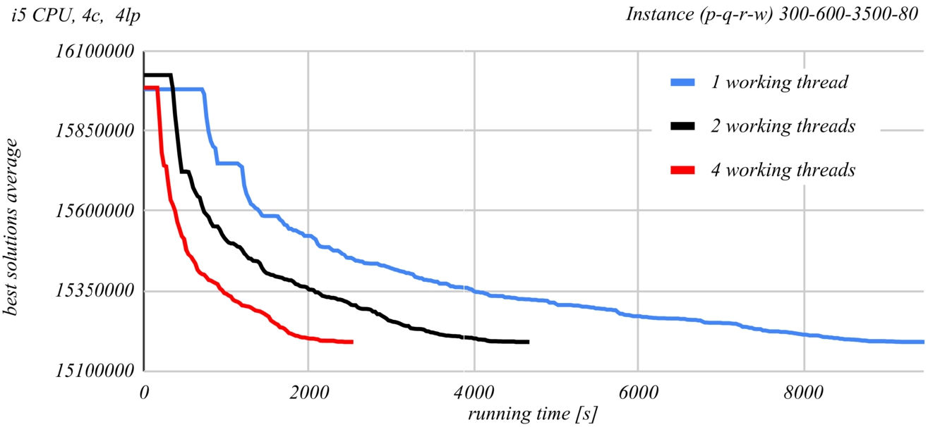
Fig. 14
Evolution of the PSDS algorithm results, when run by Intel Xenon processor.
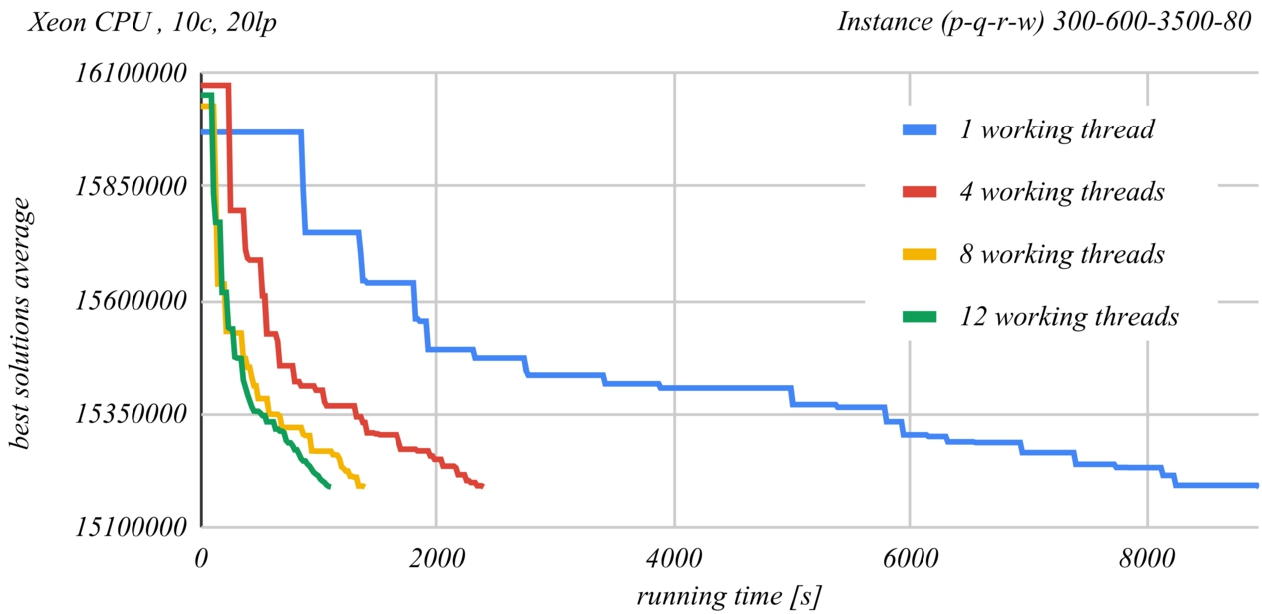
Figures 13 and 14 show a comparison of the time evolution of the solutions found by the PSDS algorithm according to the number of used worker threads. The Intel Core i5-4590 CPU at 3.3 GHz was used in the case of Fig. 13 and the Intel Xenon Silver 4114 CPU at 2.2 GHz was used in the case of Fig. 14. Each graph represents the average of the best found solution as a function of the running time, when using a certain number of worker threads. At least ten runs of the second last instance from Table 2 were performed for each of the graphs. The graphs demonstrate the effectiveness of parallel processing. The time required to obtain the same result roughly halves when doubling the number of worker threads.
6Conclusions
This study suggests an effective and fast constructive parallel heuristic algorithm whose purpose is to solve the two-stage transportation problem with fixed-charges for opening the distribution centres, which generates an essential design for the distribution system from manufacturers to customers via the DCs.
Our parallel solution approach is based on reducing of the solutions search domain to a subdomain with a reasonable size by considering a perturbation mechanism that permits us to reevaluate abandoned solutions that could conduct to optimal or sub-optimal solutions. Our approach is designed for parallel environments and takes advantage of the multi-core processor architectures.
The achieved computational results on two sets of instances from the existing literature: the first one consisting of 20 medium size benchmark instances and the second one consisting of 8 large size benchmark instances prove that our suggested innovative method is remarkably competitive, and surpasses in terms of execution time the other existing solution approaches meant for providing solutions to the TSTPFC for opening the DCs, allowing us to solve real-world applications in reasonable computational time.
Here are some significant characteristics of the method we suggest: it is designed for parallel environments and takes advantage of the new multi-core processor architectures; it is based on the reduction of the solution search domain to a subdomain with a reasonable size by considering a perturbation mechanism that permits us to reevaluate abandoned solutions that could conduct to optimal or sub-optimal solutions; it is extremely effective, offering outstanding solutions to all the instances tested and in all ten runs of the computing experiments, and it can be adapted easily to various supply chain network design problems, proving its flexibility.
References
1 | Buson, E., Roberti, R., Toth, P. ((2014) ). A reduced-cost iterated local search heuristic for the fixed-charge transportation problem. Operations Research, 62(5): , 1095–1106. |
2 | Calvete, H., Gale, C., Iranzo, J. ((2016) ). An improved evolutionary algorithm for the two-stage transportation problem with fixed charge at depots. OR Spectrum, 38: , 189–206. |
3 | Calvete, H., Gale, C., Iranzo, J., Toth, P. ((2018) ). A matheuristic for the two-stage fixed-charge transportation problem. Computers & Operations Research, 95: , 113–122. |
4 | Cosma, O., Danciulescu, D., Pop, P.C. ((2019) ). On the two-stage transportation problem with fixed charge for opening the distribution centers. IEEE Access, 7: , 113684–113698. |
5 | Cosma, O., Pop, P.C., Danciulescu, D. ((2020) ). A novel matheuristic approach for a two-stage transportation problem with fixed costs associated to the routes. Computers & Operations Research, 118: , 104906. |
6 | Cosma, O., Pop, P.C., Matei, O., Zelina, I. ((2018) ). A hybrid iterated local search for solving a particular two-stage fixed-charge transportation problem. In: Hybrid Artificial Intelligent Systems, HAIS 2018, Lecture Notes in Computer Science, Vol. 10870: , pp. 684–693. |
7 | Gen, M., Altiparmak, F., Lin, L. ((2006) ). A genetic algorithm for two-stage transportation problem using priority based encoding. OR Spectrum, 28: , 337–354. |
8 | Guisewite, G., Pardalos, P. ((1990) ). Minimum concave-cost network flow problems: applications, complexity, and algorithms. Annals of Operations Research, 25(1): , 75–99. |
9 | Hundt, R. (2011). Loop Recognition in C++/Java/Go/Scala. In: Proceedings of Scala Days 2011. https://days2011.scala-lang.org/sites/days2011/files/ws3-1-Hundt.pdf. |
10 | PassMark (2020). CPU Benchmarks. https://www.cpubenchmark.net/compare/Intel-Pentium-D-830-vs-Intel-i5-4590/1127vs2234. |
11 | Pirkul, H., Jayaraman, V. ((1998) ). A multi-commodity, multi-plant, capacitated facility location problem. Formulation and efficient heuristic solution. Computers & Operations Research, 25(10): , 869–878. |
12 | Pop, P.C., Matei, O., Pop Sitar, C., Zelina, I. ((2016) ). A hybrid based genetic algorithm for solving a capacitated fixed-charge transportation problem. Carpathian Journal of Mathematics, 32(2): , 225–232. |
13 | Pop, P.C., Sabo, C., Biesinger, B., Hu, B., Raidl, G. ((2017) ). Solving the two-stage fixed-charge transportation problem with a hybrid genetic algorithm. Carpathian Journal of Mathematics, 33(3): , 365–371. |
14 | Raj, K.A.A.D., Rajendran, C. ((2012) ). A genetic algorithm for solving the fixed-charge transportation model. Two-stage problem. Computers & Operations Research, 39(9): , 2016–2032. |
15 | Trobec, R., Slivnik, B., Bulic, P., Robic, B. ((2018) ). Introduction to Parallel Computing. From Algorithms to Programming on State-of-the-Art Platforms. Springer, Switzerland. |


