
Long Short-Term Memory Networks for Traffic Flow Forecasting: Exploring Input Variables, Time Frames and Multi-Step Approaches
Abstract
Traffic flow forecasting is an acknowledged time series problem whose solutions have been essentially grounded on statistical-based models. Recent times came, however, with promising results regarding the use of Recurrent Neural Networks (RNNs), such as Long Short-Term Memory networks (LSTMs), to accurately address time series problems. Literature is, however, evasive in regard to several aspects of the conceived models and often exhibits misconceptions that may lead to important pitfalls. This study aims to conceive and find the best possible LSTM model for traffic flow forecasting while addressing several important aspects of such models such as the multitude of input features, the time frames used by the model and the employed approach for multi-step forecasting. To overcome the spatial problem of open source datasets, this study presents and describes a new dataset collected by the authors of this work. After several weeks of model fitting, Recursive Multi-Step Multi-Variate models were the ones showing better performance, strengthening the perception that LSTMs can be used to accurately forecast the traffic flow for several future timesteps.
1Introduction
Recent years have been undoubtedly beneficial to the machine learning community. Deep learning, in particular, has assumed a prominent position in many distinct fields such as computer vision (Karpathy et al., 2014; Zhang et al., 2016), speech recognition (Graves et al., 2013; Trianto et al., 2018), or natural language processing (Zhang et al., 2017; Huang et al., 2018), just to name a few. This is the result of the increased robustness and ability to generalize that deep learning models have achieved as well as the appearance of new application-specific integrated circuits, such as Tensor Processing Units (TPUs) or Graphics Processing Units (GPUs), with superior capacities.
Time series problems are among those who have benefited from the progress of deep learning. In its essence, a time series problem consists in forecasting future values based on a set of previous observations, ordered in time. Indeed, there are an endless number of time series problems, with the major constraint being the availability of past observations. Until recently, the main focus was on using statistical-based models such as the AutoRegressive Integrated Moving Average (ARIMA) or ARIMA with Explanatory Variable (ARIMAX) to forecast future points (Babu and Reddy, 2012; Cortez et al., 2004). However, the results produced by such models have now been superseded by those produced by deep learning ones, in particular by Recurrent Neural Networks (RNNs) (Fernandes et al., 2019; Fu et al., 2016; Zhao et al., 2017). The promise of RNNs is that the temporal dependence and contextual information in the input data can be learned and generalized to produce reliable forecasts. Long Short-Term Memory networks (LSTMs), a specific type of RNNs, are among those that have been showed to produce valid results on time series data (Zhao et al., 2017; Ma et al., 2015).
An important time series problem is related to traffic flow forecasting. Indeed, in our days, road safety has become a major concern of our society. This fact is easily explained with the substantial number of deaths happening on the roads every day. Hence, the possibility of knowing beforehand how the traffic flow will change in the next minutes or hours would enable a driver to opt for a different road, a cyclist to opt for another hour to go cycling or a pedestrian to choose a less polluted zone. Due to the difficulty of having real contemporary data, the great majority of traffic flow forecasting studies uses open datasets such as PeMS, a dataset describing the occupancy rate of different car lanes of the San Francisco bay area. However, the use of such datasets raises some constraints. The first one is related to the different characteristics of traffic in distinct countries, cities and roads, i.e. a model that has been conceived over California roads is likely to behave poorly in other countries and cities. Secondly, the lack of real time data prevents the models from being, indeed, deployed and used to forecast the traffic flow in a real life scenario. Differently, we developed a software artefact, entitled as The Collector, that, among others, has been collecting real traffic data, uninterruptedly, since the 2018 in demarcated regions. This allows us to tackle both issues. The challenges, however, remain the same. On the one hand, traffic flow manifests a stochastic non-linear nature. On the other, some conception pitfalls are recurrent. Indeed, there seems to be a misconception about the importance of an adequate forecasting architecture and the tuning of LSTM or ARIMA models in regard to the used time frames. Moreover, existing models do not clearly describe the method that was used for multi-step forecasting, which may be indicative of prediction errors. Therefore, this work makes use of the dataset produced by The Collector to conceive ARIMA and state-of-the-art LSTM models to answer the following research questions:
1. Do LSTM networks have better accuracy than statistical-based models for traffic flow forecasting?
2. Are LSTM networks capable of accurately forecasting the traffic flow of a road for multiple future timesteps (multi-step)?
3. Do recursive multi-step LSTM networks have better accuracy than multi-step vector output ones?
4. Do multi-variate LSTM networks have better accuracy than uni-variate ones?
The remainder of this paper is structured as follows, i.e. the next section describes the current state of the art, the ARIMA and LSTMs models as well as the importance of spatial-temporal dependencies in time series; the subsequent section includes a description of the used materials, the implemented methods and the software developed for data collection; later, the performed experiments are explained, with results being gathered and analysed; finally, conclusions are drawn.
2State of the Art
Traffic flow forecasting has been in the mind of researchers for the last decades, with the initial approach being focused on statistical-based models. However, recent times have come with very promising results in regard to the use of RNNs to accurately address time series problems.
2.1ARIMA Models and LSTM Networks
ARIMA is a forecasting algorithm originally developed by Box and Jenkins (1976). It belongs to a class of uni-variate auto-regressive algorithms used in forecasting applications based on time series data. ARIMA models are generally defined by the tuple (q, d, p), where q is the order of the auto-regressive components; d is the number of differencing operators; and p is the highest order of the moving average term. These parameters control the complexity of the model and, consequently, the auto-regression, integration and moving average components of the algorithm (Van Der Voort et al., 1996), i.e.:
(1)
• y denotes a general time series;
•
•
•
•
•
The Auto-Regressive Integrated Moving Average with Explanatory Variable (ARIMAX) model is considered an ARIMA extension to a multiple variable (multi-variate) problem. It is a multiple regression model with autoregressive (AR) and moving average (MA) terms. Taking in consideration a different representation of the ARIMA
(2)
The expression
(3)
On the other hand, recent times come with very promising results in regard to the use of RNNs (Ma et al., 2015; Fernandes et al., 2019). As opposed to classical Artificial Neural Networks (ANNs), RNNs allow information to persist due to its recurrence and chain-like nature, i.e. previous information can be connected to the present. The promise of RNNs, and LSTMs in particular, is that the temporal dependence and contextual information in the input data can be learned. LSTMs were introduced in 1997, by Hochreiter and Schmidhuber (1997), but many more contributed to the current state-of-the-art (Gers et al., 2000; Bayer et al., 2009). LSTMs are a type of RNNs capable of learning long and short-term temporal dependencies. LSTM computational units are called memory cells (or neurons). The key factor of these cells is the fact that they are stateful, i.e. they contain cell state. In addition, unlike typical RNNs, each memory cell of an LSTM contains four neural network layers interacting with each other. These network layers, also known as gates, give the LSTM the ability to further govern the information flow, i.e. to forget or include information into the cell state. Gates are composed of a sigmoid neural network layer, which specifies how much information the cell wants to forget (
• The forget gate,
• The input gate,
• The output gate,
From this base some variants have emerged (Greff et al., 2017). The main differences refer, in essence, to the presence/absence of different gates or to the input of each one. Due to its characteristics, LSTMs have achieved remarkable results in sequence problems such as text classification (Breuel, 2017; Chenbin et al., 2018), music generation (Coca et al., 2013; Choi et al., 2016), handwriting recognition (Pham et al., 2014; Messina and Louradour, 2015) or speech recognition (Graves et al., 2013; Sak et al., 2014), just to name a few. Traffic forecasting is yet another domain where LSTMs have been applied successfully (Tian and Pan, 2015; Fu et al., 2016; Cui et al., 2018). Indeed, many studies have already engaged on comparing the performance and accuracy of ARIMA and LSTM models for traffic flow forecasting, with LSTMs outperforming ARIMA models (Ma et al., 2015; Fu et al., 2016; Zhao et al., 2017), even in the presence of data-scarce environments (Fernandes et al., 2019). In Fu et al. (2016), the authors conceived a LSTM model over the PeMS dataset to predict short-term traffic flow, showing that LSTM had a slightly better performance when compared to ARIMA. Another study focused on short-term traffic flow is the one performed by Zhao et al. (2017) where these authors propose a model applied over data collected by the Beijing Traffic Management Bureau, where LSTM proved to behave better than ARIMA, specially for long forecast windows. On the other hand, Ma et al. (2015) proposed an LSTM model to capture nonlinear traffic dynamics. Again, LSTM outperformed both classical RNNs and Support Vector Machine (SVM) models.
2.2The Importance of Spatial-Temporal Dependencies in Time Series
Intuition is enough to understand how space affects traffic flow forecasts, a stochastic non-linear time series problem. No two countries are the same, no two cities are the same and no two roads are the same. A model will lack the ability to generalize to roads that have distinct traffic patterns. Hence, it becomes extremely difficult, not to say unfeasible, to deploy a model to predict the traffic of several roads of a specific city when the model was trained on data from California roads. To deploy accurate solutions that make real-time predictions, the model needs to have information on the space it is operating. Therefore, possible solutions would include the conception of road-specific models or the categorization of roads that share similar patterns. Another possibility, even though computationally heavier, would be to create a multi-variate multi-road model receiving, as input, multiple observations from different roads at the same timestep. This work, as explained ahead, presents road-specific models that are able to provide, at any time, traffic flow forecasts of a road for each one of the subsequent twelve hours.
LSTMs are specially useful for time series problems (Gers et al., 2002). In typical ANNs, when tuning the network, the goal is typically to find the best set of hyperparameters that provide the best accuracy. It is usual to find models that have been tuned in regard to their depth, the number of neurons, the learning rate used by the optimizer or the activation function. However, in time series problems, special attention should be given to all parameters that are related to time. Tuning such parameters assumes, as demonstrated by our experiments, an increased importance.
There are essentially two main parameters to consider. The first is the number of timesteps that will compose an input sequence. This assumes critical importance when performing backpropagation through time (BPTT). BPTT is a gradient-based technique that unfolds a RNN in time to find the gradient of the cost, allowing LSTMs to learn from input sequences of timesteps (Werbos, 1990). Consider, for example, an hourly dataset: if it is defined that each input sequence is composed of twelve timesteps, it means that each input sequence will correspond to twelve hours. If we set this value to twenty-four, then it will correspond to an entire day being used when applying BPTT. Longer input sequences were problematic for classical RNNs mainly due to the vanishing and the exploding gradient problems (Hochreiter, 1998). LSTMs, on the other hand, are able to handle longer sequences with success (Hochreiter and Schmidhuber, 1997). Alternatively, it is possible to use a truncated version of BPTT (TBPTT), which limits the number of used timesteps when calculating the gradient (Elman, 1990). A second parameter that may influence a model’s performance is related to the reset frequency of the internal states of a memory cell. Indeed, as explained before, memory cells are stateful. However, different libraries handle these states differently. For instance, by default, Keras assumes that all internal states are reset after each batch. If one aims to maintain state between batches, one must explicitly define such behaviour. Usually, such behaviour is useful when it is assumed that information from past sequences may be useful to future sequences. Hence, some logic should be applied so that the model may understand patterns between input sequences and how they relate to each other. There is no obvious rule of thumb but some experimentation may be performed to find a tuned value for the problem, and data, in hands.
Finally, it should be noted that the goal of any model is to provide accurate and reliable forecasts. Hence, models could be conceived to be single-step, i.e. provide a single forecast for the next immediate timestep, or multi-step, i.e. provide a set of forecasts for several future timesteps. Using the hourly dataset example, a single-step model that receives twelve input timesteps will give a prediction for the thirteenth timestep. A multi-step model would give forecasts for the thirteenth, fourteenth and fifteenth timesteps, for example. If single-step models are fairly easy to conceive and evaluate, multi-step models are, on the other hand, harder. In essence, there are two main options to consider when conceiving multi-step models. The first is to have as many neurons in the output layer of the model as timesteps to forecast (Multi-Step Vector-Output). Hence, if one aims to forecast three future timesteps the model would have three output neurons. The second option would be to conceive a single-step model and recursively call it for as many future timesteps as one aims to forecast (Recursive Multi-Step). Again, as an example, let us consider the hourly dataset and an input sequence of twelve timesteps. First, we would conceive the model as single-step, i.e. the model would receive twelve hours as input and would output the thirteenth hour. Then, we would evaluate its performance, i.e. how accurate is the model in forecasting the thirteenth timestep. We would then push the predicted value of the thirteenth timestep to the input sequence, remove the oldest timestep (to ensure that the input sequence consists of twelve timesteps) and give the updated input sequence to the model to get the forecast of the fourteenth timestep. We would keep repeating this process until the forecasting horizon is reached. This is what we call a blind prediction using a Recursive Multi-Step approach. Obviously, this strategy suffers from the accumulation of errors with higher forecasting horizons (Zheng et al., 2017). However, there is no other valid way to evaluate such a model since the only way to know multiple future values is by using predictions of the future itself. Literature is evasive in regard to the used methodology for forecasting. Nonetheless, as we show in the next sections, even though Multi-Step Vector-Output models are easier to conceive and evaluate, Recursive Multi-Step models are better, both in terms of accuracy as well as computational performance.
2.3The Literature
Recent studies have emerged where LSTM networks are used for traffic flow forecasting. However, it is possible to verify that many exhibit flaws and leave untreated several important aspects of LSTMs.
In Fu et al. (2016), the authors conceived two distinct RNN models for short-term traffic flow prediction over the PeMS dataset. Their experiments were based on an input sequence of six timesteps of five minutes each (thirty minutes) to predict the traffic flow for the next five minutes (single-step). No experimentation was performed in order to find the optimized values for any of the time parameters. No reference is made about the update pattern of the internal state of a memory cell.
In Tian and Pan (2015), the PeMS dataset was again used to develop a LSTM model for short-term traffic flow prediction. The focus is again to develop a single-step model. However, several figures depict predictions for a time window far superior (one day) without any explanation on the method that was used to evaluate this multi-step model. On the other hand, the authors clarify the features provided as input to the model. The authors opted to tune the number of memory cells of each layer and the size of the input layer. In regard to this last parameter, it is expected that the authors are indeed referring to the input shape of the first LSTM layer. Hence, the authors are tuning the number of timesteps that make an input sequence. All values from one to twelve were tried, meaning, in the first case, a sequence with just one timestep (five minutes of data) and, in the last case, a sequence with twelve timesteps (one hour of data). It would be interesting to know if blind recursive multi-step forecast was performed.
In Cui et al. (2018), the authors propose a deep stacked bidirectional LSTM in order to consider both forward and backward dependencies in time series data. Their goal is to predict traffic speed using two distinct datasets, even though later the authors claim that only one was used to evaluate the model. To fully capture the spatial dimension of the problem, and since the dataset contains observations of multiple roads, the authors opted to develop a multi-variate multi-road model receiving, as input, multiple observations from different roads at the same timestep, as discussed before. Each input sequence is composed of ten timesteps of five minutes, with a prediction being provided for the subsequent timestep (single-step). The number of timesteps in the input sequence was set as six, eight, ten, and twelve timesteps. The obtained results were very similar, which can be explained by the fact that all the attempted values are also very close. Indeed, it would be interesting to know how would the model behave with higher input timesteps that could represent, for example, an entire day instead of a few tens of minutes. No reference is made about the update pattern of the internal state of a memory cell.
Another work, performed by Zheng et al. (2017), leaves aside traffic and focuses on electric load forecasting using a uni-variate dataset collected by the authors. Interestingly, the authors of this work clearly describe the multi-step forecasting concept, having used a forecasting horizon of ninety-six timesteps. Such a long forecasting horizon directly affects the accuracy of the model. Nonetheless, the authors found that LSTM still outperformed traditional forecasting methods, such as SARIMA. On the other hand, input sequences were composed of ten days of timesteps. There are no details regarding how was this value found and if any experimentation was performed.
Other studies focus on different deep learning models for time series forecasting. Indeed, new trends are emerging regarding the use of Convolutional Neural Networks (CNNs) (Cai et al., 2019; Rahimilarki et al., 2019; Yao et al., 2017) and attention mechanisms (Serra et al., 2018; Vaswani et al., 2017). One study, performed by Cai et al. (2019), focused on deep learning-based techniques, in particular RNNs and CNNs, for day-ahead multi-step load forecasting in commercial buildings, comparing the obtained results with ARIMAX. The gated 24-h CNN model was the one achieving the best results, improving ARIMAX accuracy by 22.6%. A different study, performed by Yao et al. (2017), integrated, in a platform called DeepSense, both CNNs and RNNs, where the input sensor measurements were prepared as a time series. The CNN was responsible for learning intra-interval interactions, with the intra-interval representations along time being inputted to the RNN. Rahimilarki et al. (2019) proposed a deep learning fault detection approach based on CNNs, with the goal being to diagnose anomalies in the output of wind turbine systems. Time-series data was converted as 2D images and fed to the conceived CNNs, with deeper CNNs outperforming shallow ones. On the other hand, attention mechanisms, initially applied to machine translation (Bahdanau et al., 2015), have been growing in popularity for time series forecasting. Indeed, Vaswani et al. (2017) propose a Transformer that is solely based on attention mechanisms, discarding recurrence and convolutions. Such mechanisms allow the model to selectively focus on parts of the source data, which may be important when handling longer input sequences. For instance, a study performed by Serra et al. (2018) used convolutional attention mechanisms based on the temporal output of CNNs, to conceive a network able to convert variable-length time to fixed-length low-dimensional time series data representation.
3Materials and Methods
The next lines describe the materials and methods used in this work, including the collected dataset and all the applied treatments, the evaluation metrics, and the used technologies. The dataset used in this study is available, in its raw state, in an online repository (github.com/brunofmf/Datasets4SocialGood), under a MIT license.
3.1Data Collection
The dataset used in this work was created from scratch and contains real world data. A software artefact, entitled as The Collector, was developed to collect data from a set of public APIs. In particular, TOMTOM Traffic Flow API was the one used to create the traffic dataset, which has, as features, the city name, the road name, the functional road class describing the road type, the current speed in km/h at the observed road, the free flow speed in km/h expected under ideal free flow conditions, the speed_diff that corresponds to the difference between the speed that is expected under ideal conditions at the road and the speed that is being currently observed at that same road, the current travel time in seconds, the travel time in seconds which would be expected under ideal conditions, the time_diff that corresponds to the difference between the travel time that is expected under ideal conditions at the road and the travel time that is being currently observed at that same road, and a timestamp. Several other APIs complement the dataset, including the Open Weather Maps API which returns the weather description, temperature, atmospheric pressure, wind speed and precipitation volumes, among others. Pollution data is also available but was discarded for this study. Table 1 summarizes all the available features.
Table 1
Availablefeatures in the traffic and weather datasets.
| # | Features | Description | |
| Traffic dataset | 1 | city_name | Name of the city the road belongs to |
| 2 | road_num | Road identification number | |
| 3 | road_name | Road name | |
| 4 | functional_road_class | Road category description | |
| 5 | current_speed | Current speed observed at the road (km/h) | |
| 6 | free_flow_speed | Speed expected under ideal conditions (km/h) | |
| 7 | speed_diff | Speed difference (#6–#5) | |
| 8 | current_travel_time | Current travel time observed at the road (s) | |
| 9 | free_flow_travel_time | Travel time expected under ideal conditions (s) | |
| 10 | time_diff | Time difference (#9–#8) | |
| 11 | creation_date | Timestamp (YYYY-MM-DD HH24:MI:SS) | |
| Weather dataset | 1 | city_name | Name of the city the road belongs to |
| 2 | weather_description | Textual description of the weather | |
| 3 | temperature | In celsius | |
| 4 | atmospheric_pressure | Atmospheric pressure on the sea level (hPa) | |
| 5 | humidity | In percentage | |
| 6 | wind_speed | In meter/second | |
| 7 | cloudiness | In percentage | |
| 8 | precipitation | Precipitation volume for the last hour (mm) | |
| 9 | current_luminosity | Current luminosity (categorical) | |
| 10 | sunrise | Sunrise time (unix, UTC) | |
| 11 | sunset | Sunset time (unix, UTC) | |
| 12 | creation_date | Timestamp (YYYY-MM-DD HH24:MI:SS) |
The software went live on 24th July 2018 and has been collecting data uninterruptedly. It works by making an API call every twenty minutes using an HTTP Get request. It parses the received JSON object and saves the records on the database. The software was made so that any road of any city or country can be easily added to the fetch list. As of June 2019, the database contains, approximately, ten million records for several roads of several cities.
3.2Data Preparation and Pre-Processing
Two distinct datasets were available, namely the traffic and the weather ones (Table 1). Both datasets include observations from 24th July 2018 to 30th April 2019, in twenty minutes intervals, of several Portuguese cities. Among all the available features, speed_diff is the one that will be used to quantify traffic. Indeed, this feature corresponds to the difference between the speed, in km/h, that is expected under ideal conditions in a road and the speed, in km/h, that is being currently observed at that same road. Hence, high speed_diff values mean that one is going much slower than what would be expected at that road, while low values mean that one is going almost at the ideal speed. For example, a speed_diff of zero means no traffic for that road while a value of 40 km/h means that one is going 40 km/h slower than expected.
The first step to prepare both datasets was to focus on a specific road of the city of Braga, in Portugal, and filter out the remaining cities and roads. Then, in regard to the traffic dataset, features that were static, such as the road_name and the functional_road_class, were removed. The time_diff, free_flow and current_speed features, which are highly correlated with the speed_diff, were also filtered out. Regarding the weather dataset, the only considered features were, besides the city_name and creation_date, the temperature and precipitation. Afterwards, for both datasets, six new temporal and contextual features were created based on the creation_date of each observation. The year, month, day, week_day, hour and minutes were the created features. The minutes feature was further normalized to have one of three possible values: 0, 20 or 40. Hence, all observations with minutes between
Table 2
Features present in the final dataset.
| # | Features | Observation example |
| 0 | timestep index | 2019-04-23 17:40 |
| 1 | speed_diff | 32 |
| 2 | temperature | 10 |
| 3 | precipitation | 0 |
| 4 | week_day | 1 |
| 5 | hour | 17 |
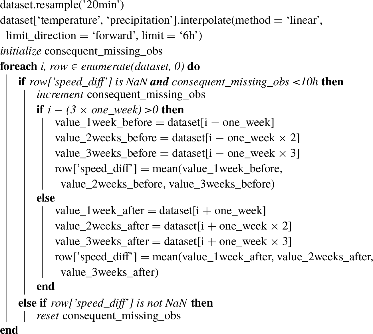
No missing values were present. However, due to API limitations or to the fact that The Collector was down, there are missing timesteps/observations. In a time series problem, missing timesteps may lead to the creation of incorrect patterns in input sequences. Consider, for example, the situation where a sequence contains observations for the fourth, fifth and sixth hours of a day and then, due to the nonexistence of observations, it is followed by the fourteenth and fifteenth hours of that same day. This sequence would not describe the traffic pattern of the road. Hence, different approaches can be followed to solve this situation. The approach followed in this work was to first include all missing timesteps with NaN (Not a Number). Missing values, filled with NaN, were interpolated when the amount of consecutive missing observations corresponded to less than six hours for weather features and less than ten hours for traffic features. Weather features (temperature and precipitation) were linearly interpolated. On the other hand, speed_diff, the only traffic feature, was computed based on the mean value of that same timestep at the three previous weeks. The dataset was iterated, observation by observation, from the oldest to the newest. In the case there was no information about the three previous weeks, the next three weeks were the ones used. In the case of timestep gaps longer than ten hours, the entire day would be removed. Algorithm 1 describes the function that was developed for the computation of missing timesteps.
Algorithm 1
Computation of missing timesteps.
Considering that LSTMs work internally with the hyperbolic tangent function (tanh), the decision was to normalize all features so that they would fit into the interval
(4)
Finally, due to computational constraints, the dataset was grouped by hour. The final multi-variate dataset contained 5050 observations, with a shape of
3.3From an Unsupervised to a Supervised Problem
The dataset was now a single sequence of 5050 ordered timesteps. However, it was still not ready to be used by LSTM models. Indeed, in order to create such models one is required to set the problem as a supervised one, with inputs and corresponding labels. Hence, data was divided into smaller sequences, with its length depending on the number of input timesteps to be used. The label of each new sequence was the next immediate timestep, or a sequence of timesteps, depending if the model was to be Single-Step and Recursive Multi-Step, or Multi-Step Vector-Output, respectively (Algorithm 2).
Algorithm 2
From an unsupervised to a supervised problem.
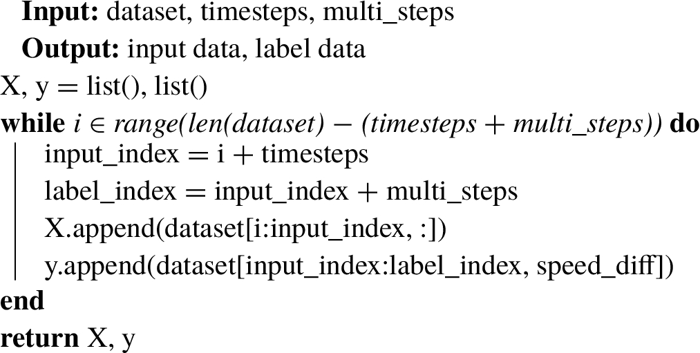
Consider the scenario of a single-step model that receives the last twenty-four hours of traffic and predicts how the traffic will change in the next hour. In this scenario, the initial dataset with 5050 ordered timesteps will be divided into smaller sequences of 24 timesteps, i.e. the length of the input sequence. Being this a single-step model, or a recursive multi-step one, the label will be composed of just one timestep and will have the value of the timestep that follows the twenty-fourth one. A sliding window over the initial dataset is used to create batches of sequences and labels. At the end, the dataframe (a Pandas’ object), will have a shape of (5025, 24, 5), where the first element dimension corresponds to the number of samples, the second, to the number of input timesteps, and the third, to the number of features.
3.4Technologies and Libraries
Python, version 3.6, was the used programming language for data preparation and pre-processing as well as for model development and evaluation. Pandas, NumPy, scikit-learn, matplotlib and statsmodels were the used libraries. Tensorflow v1.12.0 was the machine learning library used to conceive the deep learning models. tf.keras, TensorFlow’s implementation of the Keras API specification, was also used. For increased performance, and to fit the models in reasonable times, Tesla T4 GPUs were used as well as an optimized version of LSTMs using CuDNN (CudnnLSTM), NVIDIA’s deep neural network library of primitives for deep neural networks. It is worth mentioning that this hardware was made available by Google’s Colaboratory, a free python environment that requires minimal setup and runs entirely in the cloud.
3.5Evaluation Metrics
To evaluate the effectiveness of the candidate models, two error metrics were used. The first one corresponds the Root Mean Squared Error (RMSE). This allows us to penalize outliers and easily interpret the obtained results since they are in the same unit of the feature that is being predicted by the model. Its formula is as follows:
(5)
The second error metric corresponds to the Mean Absolute Error (MAE). It was mainly used to complement and strengthen the confidence on the obtained values. Its formulas is as follows:
(6)
All candidate models were evaluated in regard to the mentioned metrics. A time series cross-validator was also used to provide train/test indices to split time series data samples. In this case, the kth split returns the first k folds as train set and the
4Experiments
The main goal of this study is to develop and tune a deep learning model, in particular a LSTM neural network, to forecast the traffic flow. This is achieved by forecasting the speed_diff feature. The higher the speed_diff value the heavier the traffic. All models were conceived as multi-step, i.e. to forecast twelve consecutive hours.
Due to the random initialization of LSTM weights, three repetitions of each combination of parameters were performed on incremental sets of data, taking the mean of RMSE and MAE to verify the model’s quality. Several experiments were performed to find the best set of parameters for the final model. More than finding the optimized set of hyperparameters, such experiments aim to study and evaluate the nature and architecture of LSTMs in regard to the shape of its output, the multitude of used features, and the ability to forecast multiple future timesteps. An experiment was also set where ARIMA models are deployed, evaluated and later compared with LSTMs.
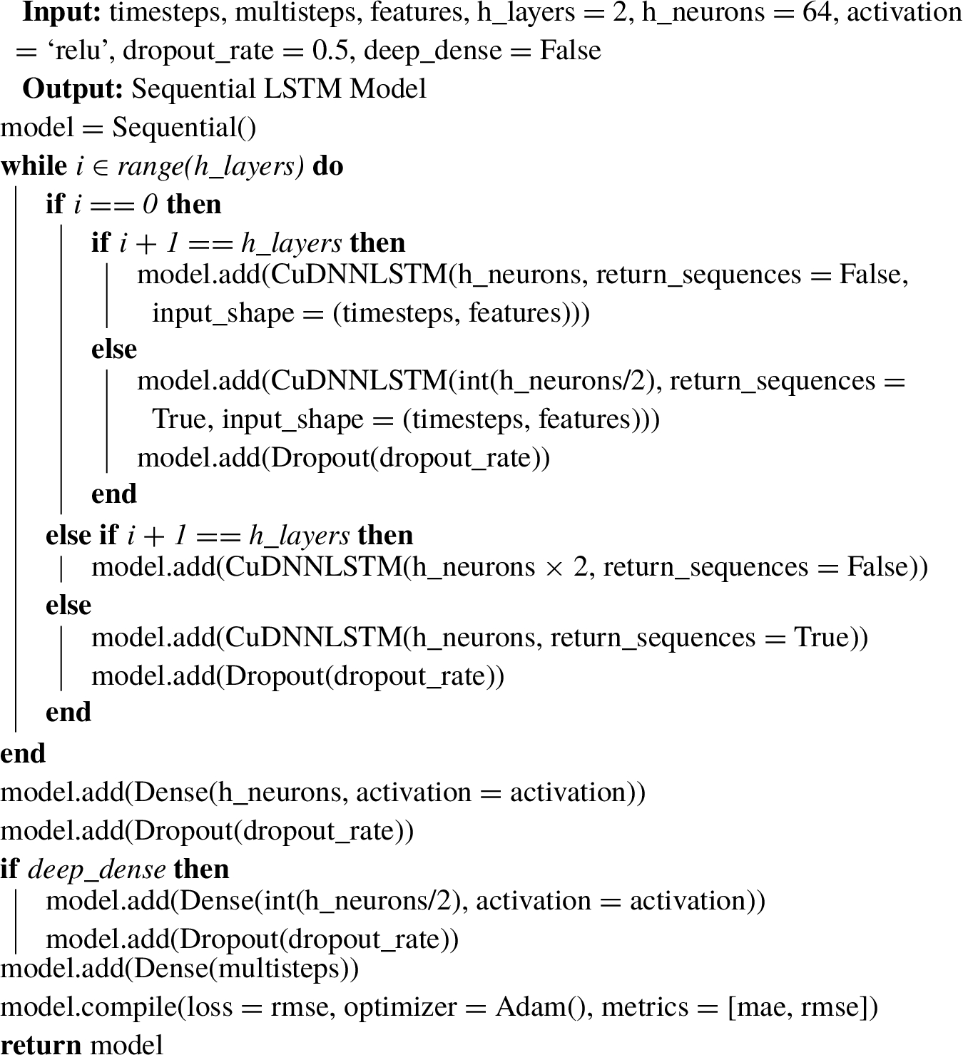
Algorithm 3 details the generic function that was written for the conception and compilation of the candidate LSTM models. This function is used in all LSTM experiments, with the inputs of the function defining the model’s structure and time frames.
Algorithm 3
Function for LSTM model’s conception and compilation.
4.1ARIMA and ARIMAX
When compared to LSTMs, ARIMA and ARIMAX are considered more traditional approaches to time series forecasting. In truth, they are older and based on classical mathematical regression operations. Nevertheless, there are several examples in the literature of their usage, especially in the same area of study as the one presented in this paper. Therefore, ARIMA and ARIMAX models shall be used as benchmarks for the conceived LSTMs. Hence, using the collected data, models were trained in order to mimic the conditions in which LSTM were trained, i.e. using ARIMA for uni-variate and ARIMAX for multi-variate problems. Considering both of these models, data preparation is less strict, as there is no need to turn the data into sequences. The algorithms automatically process data from the ordered dataset. The remaining data pre-processing operations were already explained.
The experiments made with the ARIMA model used a grid search approach to fine tune the
In order to tackle multi-step predictions, a forecast method was used, which allows to directly forecast a number of instances from the last point in the trained dataset. This is consistent with the blind multi-step forecasting approach. For a multi-step approach incorporating real observations, the model needs to be retrained after each dataset change. The time used to train an ARIMA or ARIMAX model is usually faster than LSTM, but in the case of forecasting one step ahead with real observations, the need for retrain at each timestep, and the number of experiments being performed, made the ARIMA and ARIMAX slower than the worst performing LSTM. For simplicity, only blind multi-step forecasting models were considered.
4.2Recursive Multi-Step vs Multi-Step Vector Output LSTMs
The goal of this experiment was to compare the performance, both computationally and in terms of accuracy, of two distinct multi-step approaches. It soon became obvious that the Multi-Step Vector Output model would require a more complex architecture. That came, however, with a significantly higher computational and training time cost. Therefore, for this experiment, only uni-variate models were considered. Both models receive input sequences of one feature, i.e. speed_diff, and provide speed_diff forecasts for the next twelve hours. Intuition and random search were used to reduce the parameter’s search space size and to find the best set of parameters for each model.
A Recursive Multi-Step LSTM model was conceived and tuned in regard to a set of parameters. As explained before, such a model forecasts the next immediate timestep, being then called recursively twelve times. RMSE and MAE values are gathered both for blind and non-blind forecasts. Non-blind forecasts use real values when iterating recursively. Obviously, non-blind forecasts produce a better result than blind ones since this last approach suffers from the accumulation of errors with higher forecasting horizons. This serves the purpose of showing that misconceptions may lead researchers to present models that have been inappropriately evaluated. Nonetheless, blind forecasts are the ones to be considered. Table 3 describes the parameter searching space considered for the candidate models.
Table 3
Recursive Multi-Step Uni-Variate parameters’ searching space.
| Parameter | Searched values | Rationale |
| Epochs |
| – |
| Timesteps |
| Input of 0.5 to 4 days |
| Batch size |
| 1 day to 4 weeks |
| LSTM layers |
| Number of LSTM layers |
| Dense layers | 1 | Number of dense layers |
| Dense activation | [ReLU, tanh] | Activation function |
| Neurons |
| For dense and LSTM layers |
| Dropout rate |
| For dense and LSTM layers |
| Learning rate | Tuned via callback | Keras callback |
| Multisteps | 12 | 12 hours |
| Features | speed_diff | Uni-variate |
| CV Splits | 3 | Time series cross-validator |
As soon as the first Multi-Step Vector Output candidate model started its training, it became obvious that, computationally, it would be much expensive and it would take a considerable amount of time to go through all searching space. Therefore, a smaller parameter space was considered (Table 4). Intuition and random search helped reduce the number of fits performed and the amount of time it took to gather results.
Table 4
Multi-Step Vector Output parameters’ searching space.
| Parameter | Searched values | Rationale |
| Epochs |
| – |
| Timesteps |
| Input of 2 and 4 days |
| Batch size |
| 1, 2 and 4 weeks |
| LSTM layers |
| Number of LSTM layers |
| Dense layers |
| Number of dense layers |
| Dense activation | [ReLU, tanh] | Activation function |
| Neurons |
| For dense and LSTM layers |
| Dropout rate |
| For dense and LSTM layers |
| Learning rate | Tuned via callback | Keras callback |
| Multisteps | 12 | 12 hours |
| Features | speed_diff | Uni-variate |
| CV Splits | 3 | Time series cross-validator |
4.3Uni-Variate vs Multi-Variate LSTMs
This experiment aimed to compare the performance, both computationally and in terms of accuracy, of uni-variate and multi-variate LSTM models. The first type, uni-variate, refers to models that use a single feature, while multi-variate ones use multiple features with the expectation of accurately generalizing the problem in hands. Both uni-variate and multi-variate models were conceived as Recursive Multi-Step. This decision was based on the fact that Recursive Multi-Step forecasting was shown to be less expensive and more accurate than Multi-Step Vector Output. Intuition and random search were, again, used to reduce the parameter’s space size and to find the best set of parameters for each model.
The model conceived for the uni-variate experiment is the same as the Recursive Multi-Step one presented in Section 4.2. Indeed, such model was already a uni-variate one, using only the speed_diff feature to recursively forecast future speed_diff values. Table 3 describes the parameter searching space considered for each candidate model.
For the multi-variate experiments, from the features considered in Table 2, temperature was removed and experiments were initially made with the speed_diff, precipitation and week_day features. Later, the hour was also added to the used features. Again, it soon became obvious that the model was becoming more expensive to train and that it was requiring a more complex architecture. However, making the model deeper came with a considerable cost in terms of the time it took for models to train. Table 5 describes the parameter searching space used for the conception of the Recursive Multi-Step Multi-Variate LSTM candidate models.
Table 5
Recursive Multi-Step Multi-Variate parameters’ searching space.
| Parameter | Searched values | Rationale |
| Epochs |
| – |
| Timesteps |
| Input of 0.5 to 4 days |
| Batch size |
| 0.5 to 4 weeks |
| LSTM layers |
| Number of LSTM layers |
| Dense layers |
| Number of dense layers |
| Dense activation | [ReLU, tanh] | Activation function |
| Neurons |
| For dense and LSTM layers |
| Dropout rate |
| For dense and LSTM layers |
| Learning rate | Tuned via callback | Keras callback |
| Multisteps | 12 | 12 hours |
| Features | speed_diff, precipitation, week_day and hour | |
| CV Splits | 3 | Time series cross-validator |
5Results and Discussion
The conceived models were evaluated in regard to the RMSE and MAE error metrics. A time series cross-validator was used to provide train and test indices to split time series data samples. The test sets were used to evaluate the model. Each training set was further split into training and validation sets in a ratio of 9:1. The results presented in the following lines are the output of a forecast function that was developed to plot and predict three entire days of the test set (72 timesteps). Mean RMSE and MAE values were computed for each prediction of each split of the time series cross-validator.
5.1ARIMA Models vs LSTM Networks
ARIMA based-models were used as a benchmark. During our analysis, it was possible to observe that ARIMA and ARIMAX models tend to be unreliable when addressing a dynamic problem such as traffic flow in an open data stream format. A different approach to data modelling could be designed, nonetheless there is no assumption or guarantee that the data will follow any specific distribution or will not be affected by outlier events.
There are issues with model training, being often impossible to train the model. Also, if the dataset of past observations is constantly updated, then there is a need to re-train models every time such events happen. So, taking into consideration the blind and real observations forecast, the latter implies that for each prediction the model needs to be re-trained. On the other hand, blind prediction needs to re-train the model each time the starting point of the prediction changes, which decreases the number of times the model needs to be re-trained even though it remains high.
Fig. 1
Two random blind multi-step forecasts for the best ARIMA and the best ARIMAX model.
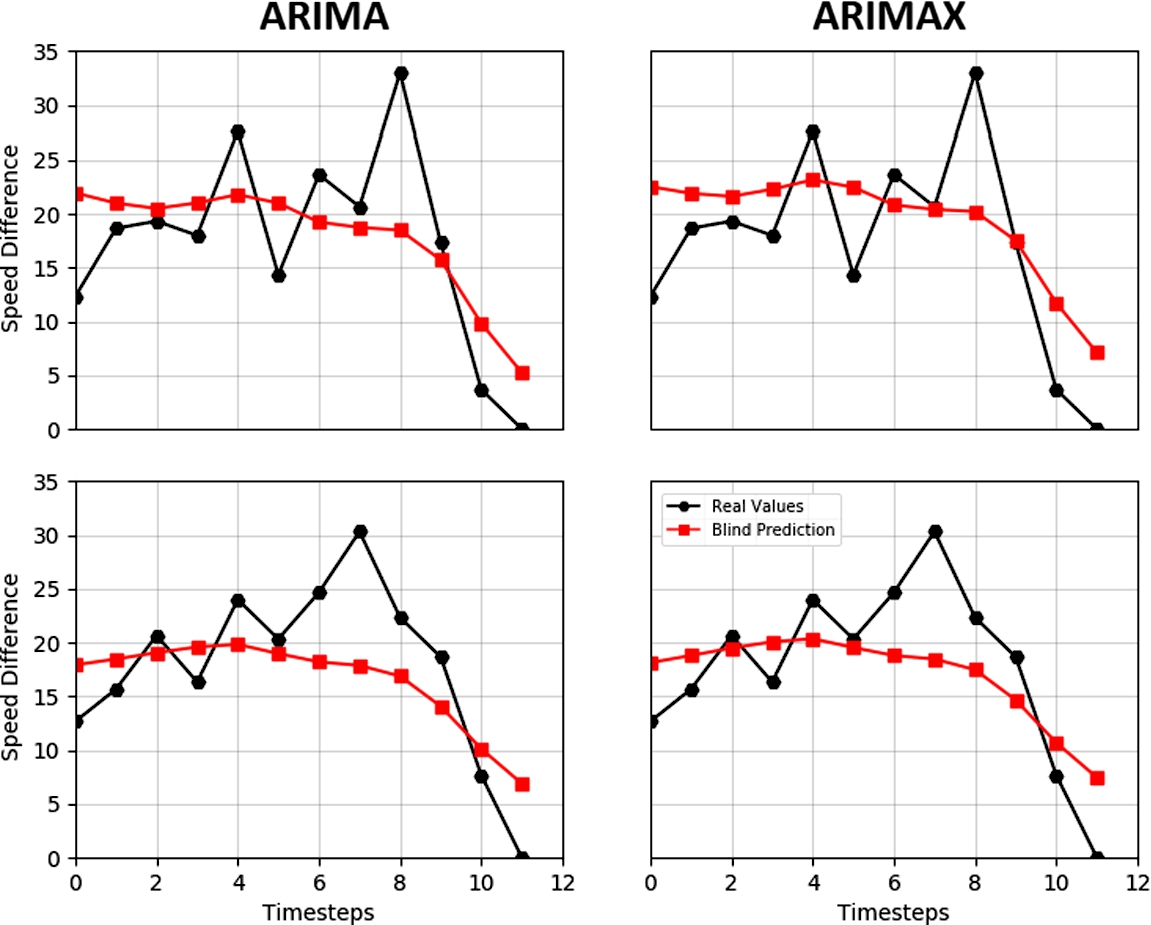
In terms of accuracy, both ARIMA and ARIMAX can yield good results for few timestep forecasts. These models behave especially badly when the series incurs, for some time, in stagnant data, i.e. when there is no speed variation for several timesteps. Figure 1 depicts some of the best multi-step forecasts using ARIMA and ARIMAX models. In Table 6, a short summary of the best model specification for both ARIMA and ARIMAX is also depicted. The higher order we achieve with the arguments
Table 6
Top-four ARIMA and ARIMAX candidate models.
| Moving average
| Dif. Operators
| Auto-regressive
| RMSE | MAE |
| ARIMA | ||||
| 12 | 1 | 2 | 6.336 | 5.088 |
| 12 | 1 | 1 | 6.452 | 5.200 |
| 8 | 1 | 2 | 7.967 | 6.275 |
| 8 | 1 | 1 | 8.869 | 7.474 |
| ARIMAX | ||||
| 12 | 1 | 2 | 6.110 | 4.918 |
| 12 | 1 | 1 | 6.171 | 4.972 |
| 8 | 1 | 2 | 8.301 | 6.822 |
| 8 | 1 | 1 | 8.325 | 6.736 |
ARIMAX behaves similarly, however the presence of contextual data makes the model slightly more accurate for each parameter configuration. On the other hand, ARIMAX models are significantly more costly to train as the computational overhead of the contextual data is directly translated to an increase in the training time. Contrary to what may be expected, ARIMAX breaks less often than the standard uni-variate ARIMA, which means that it is also more reliable for blind multi-step predictions.
When comparing ARIMA models to LSTM ones, there are some considerations to take into account. Firstly, LSTMs can achieve better forecasting performance and produce stable results despite data properties. On the other hand, ARIMA models need to enforce data to be stationary, which might not be possible in continuous streams of data. Regarding training times, ARIMA and ARIMAX have short training times but require re-training when new observations are added to the dataset and the forecast should occur after the latest observation. LSTMs do not share this problem as they can predict the next sequence of data without the need to retrain the network regardless of the starting point. This detail makes LSTMs better suited for real time applications, where trained models can deliver high accuracy results without constant need for re-train.
Other aspects, such as the presence of contextual data, benefits both approaches. Results indicate that the presence of contextual data does increase the performance of forecasts. From an analytical point of view, the major advantages of LSTM over ARIMA and ARIMAX models are its accuracy, performance, ability to train models under any data constraints, and the need to train models only once.
5.2Recursive Multi-Step vs Multi-Step Vector Output LSTMs
Both error metrics are clear when the mission is to find the best multi-step model. Recursive Multi-Step LSTM models had significantly lower RMSE and MAE values when compared to Multi-Step Vector Output ones. As depicted in Table 7, the best Recursive Multi-Step LSTM model had a RMSE of 3.496 and a MAE of 1.567 while the best Multi-Step Vector Output LSTM model had a RMSE of 5.040 and a MAE of 1.846. Indeed, after more than two hundred experiments, only one Recursive Multi-Step LSTM model had worst accuracy than the best Multi-Step Vector Output one. This leaves no room for doubt that recursive models produce significantly better models than vector output ones.
Table 7
Recursive Multi-Step vs Multi-Step Vector Output LSTMs top-five results.
| # | Timesteps | Batch | Layers | Neurons | Dropout | Act. | RMSE | MAE |
| Recursive Multi-Step Uni-Variate | ||||||||
| 209 | 96 | 672 | 5 | 64 | 0.2 | relu | 3.496 | 1.567 |
| 188 | 96 | 672 | 4 | 64 | 0.2 | tanh | 3.518 | 1.567 |
| 95 | 96 | 252 | 5 | 32 | 0.2 | relu | 3.555 | 1.592 |
| 195 | 96 | 672 | 4 | 128 | 0.5 | tanh | 3.583 | 1.598 |
| 12 | 48 | 252 | 3 | 64 | 0.5 | relu | 3.649 | 1.629 |
| Multi-Step Vector Output Uni-Variate | ||||||||
| 24 | 96 | 672 | 4 | 128 | 0.5 | relu | 5.040 | 1.846 |
| 31 | 96 | 672 | 5 | 128 | 0.2 | relu | 5.134 | 1.839 |
| 29 | 96 | 672 | 5 | 128 | 0.2 | tanh | 5.272 | 1.852 |
| 20 | 48 | 168 | 5 | 512 | 0.5 | relu | 5.279 | 1.880 |
| 30 | 96 | 672 | 5 | 128 | 0.5 | tanh | 5.325 | 1.885 |
It is worth highlighting that vector output models have as many neurons in the output layer as timesteps to forecasts. Intuitively, this would lead the model to demand a more complex architecture when compared to those that have a single neuron as output. This can be indeed verified in the performed experiments. The first round of experiments with vector output models limited the maximum number of neurons to 128 and the number of fully-connected layers to 1. This maximum number was the one used by all the best candidates. Then, the second round of experiments with vector output models considered a higher number of neurons, layers and training epochs. However, very few experiments were performed with combinations of 256 and 512 neurons, 4 and 5 hidden LSTM layers and 2 fully-connected layers. This is related to the fact that each candidate model was taking more than eight hours to train.
Fig. 2
Six random multi-step vector output forecasts of the best Multi-Step Vector Output Uni-Variate LSTM model (#24). Comparison of real values vs predicted ones using vector output forecasting.
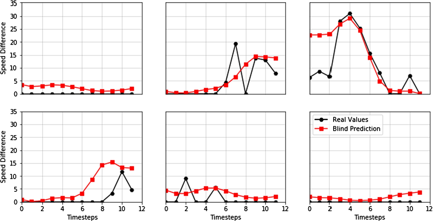
It is our conclusion that deeper and more complex architectures could improve the performance of Multi-Step Vector Output models. This comes, however, with a significant increase of training times. On the other hand, the Recursive Multi-Step LSTM models were between eight and sixteen times faster to train, required a shallower architecture and produced results that are more than 40% better. It is also interesting to note that the best models were the ones using a bigger batch size combined with input sequences of four entire days (96 timesteps). There was no clear distinction between using the rectified linear units or the hyperbolic tangent. The same argument is applied for dropout values.
Fig. 3
Six random multi-step forecasts of the best Recursive Multi-Step Uni-Variate LSTM model (#209). Comparison of real values vs predicted ones using blind forecasting vs predicted ones using known observations.
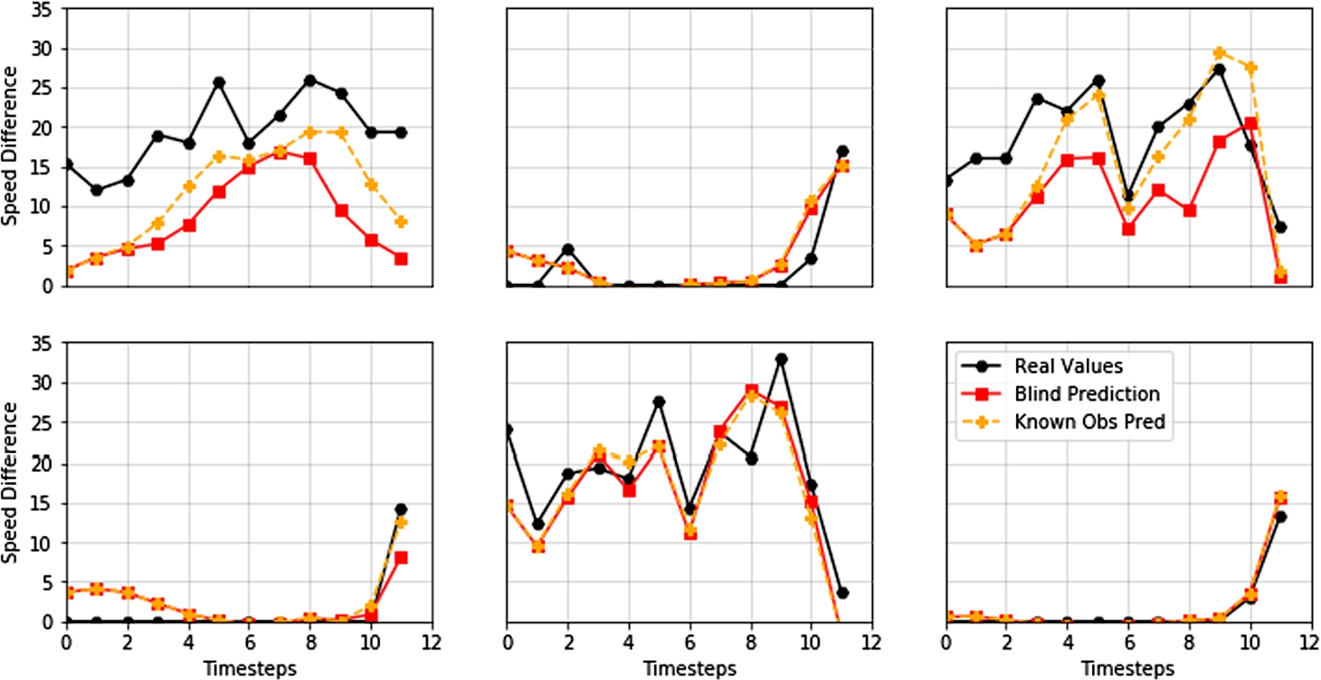
Table 7 describes the top-five results achieved with each multi-step approach. The best Recursive Multi-Step LSTM model had a RMSE of 3.496, which means that such model is able to predict, by a margin of around 3 km/h, the expected speed difference at a road for each one of the next twelve hours. These results prove the feasibility of using LSTM networks for accurate multi-step prediction. Figure 2 presents six random multi-step predictions for the best Multi-Step Vector Output LSTM model. On the other hand, Fig. 3 presents six random multi-step predictions of the best Recursive Multi-Step LSTM candidate.
5.3Uni-Variate vs Multi-Variate LSTMs
An increase of the multitude of input features led to a decrease of the RMSE and MAE values. As depicted in Table 8, the best Uni-variate LSTM model had a RMSE of 3.496 and a MAE of 1.567 while the best Multi-variate LSTM model had a RMSE of 2.907 and a MAE of 1.346, which corresponds to a decrease of more than 20% on the RMSE metric.
Table 8
Uni-Variate vs Multi-Variate LSTMs top-five results.
| # | Timesteps | Batch | Layers | Neurons | Dropout | Act. | RMSE | MAE |
| Uni-Variate Recursive Multi-Step | ||||||||
| 209 | 96 | 672 | 5 | 64 | 0.2 | relu | 3.496 | 1.567 |
| 188 | 96 | 672 | 4 | 64 | 0.2 | tanh | 3.518 | 1.567 |
| 95 | 96 | 252 | 5 | 32 | 0.2 | relu | 3.555 | 1.592 |
| 195 | 96 | 672 | 4 | 128 | 0.5 | tanh | 3.583 | 1.598 |
| 12 | 48 | 252 | 3 | 64 | 0.5 | relu | 3.649 | 1.629 |
| Multi-Variate Recursive Multi-Step | ||||||||
| 53* | 24 | 168 | 4 | 64 | 0.5 | tanh | 2.907 | 1.346 |
| 24* | 24 | 96 | 4 | 32 | 0.5 | tanh | 3.006 | 1.412 |
| 16* | 24 | 48 | 4 | 32 | 0.5 | tanh | 3.031 | 1.419 |
| 17* | 24 | 168 | 5 | 64 | 0.5 | tanh | 3.037 | 1.402 |
| 37* | 48 | 84 | 2 | 64 | 0.5 | tanh | 3.038 | 1.425 |
* Used features: speed_diff, week_day and hour.
It is worth noting that including the hour of the day as input feature allowed the model to make more accurate forecasts. On the other hand, the presence of the precipitation feature led to worst results. Moreover, it is interesting to note that the presence of more input features led to a decrease in the number of input timesteps. Indeed, the best uni-variate candidates required 96 input timesteps, while the best multi-variate ones require just 24 input timesteps. In simple terms, while the uni-variate models require four days of input to forecast the next twelve hours, the multi-variate ones require just a single day as input to forecast the same amount of hours. The batch size required by multi-variate models is also substantially lower when compared to uni-variate ones. Regarding the activation function, while there is no clear distinction between relu and tanh in uni-variate candidates, it is clear that tanh performs better in multi-variate ones with a dropout of 50%.
Even though multi-variate models took longer to train than uni-variate ones, such variation is negligible (a few tens of minutes). Moreover, the addition of more features to the model allowed it to perform better than an uni-variate one. Indeed, the addition of the hour of the day was the factor that allowed the candidate models to achieve lower error values. Table 8 describes the top-five results achieved with each approach. The best Recursive Multi-Step Multi-Variate LSTM is able to predict, by a margin inferior to 3 km/h, the expected speed difference at a road for each one of the next twelve hours. Figure 4 presents six random multi-step forecasts of the best Recursive Multi-Step Multi-Variate LSTM candidate.
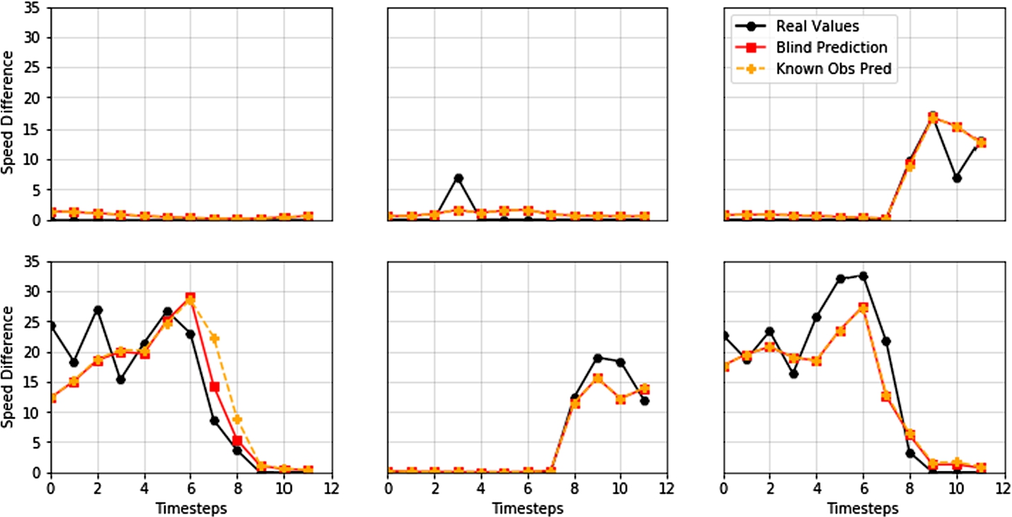
Fig. 4
Six random multi-step forecasts of the best Recursive Multi-Step Multi-Variate LSTM model (#53). Comparison of real values vs predicted ones using blind forecasting vs predicted ones using known observations.
6Conclusions
Traffic flow forecasting has been assuming a prominent position with the rise of deep learning. This is essentially happening due to the fact that state-of-the-art RNN models have now overcome previous statistical-based models, both in terms of performance as well as accuracy. From all the candidate models, and after several weeks of combined training times, the model that was able to forecast more accurately the traffic flow of a road for multiple future timesteps was the fifty-third Recursive Multi-Step Multi-Variate candidate model, with a RMSE and MAE of 2.907 and 1.346, respectively. The Uni-Variate models also presented interesting results, with its best model being 20% worst than the best Multi-Variate one. On the other hand, the best Vector Output model had a RMSE that was more than 73% worst than the best Multi-Variate model and 40% worst than the best Uni-Variate. In addition, Vector Output models took significantly more time to train when compared to the other models. The training time difference between the Uni-Variate and the Multi-Variate models can be considered negligible. On the other hand, ARIMA and ARIMAX presented results that are two times worse than the best LSTM model. In addition, the fit frequency of ARIMA models is significantly higher when compared to LSTM ones, which may be problematic in open data stream scenarios. All this is in agreement to what the literature has been presenting, confirming that these statistical-based models have now been superseded by deep learning ones. Table 9 summarizes the achieved results by each approach.
Table 9
Summary results for the best model of each approach.
| Model | RMSE | MAE |
| Recursive Multi-Step Multi-Variate | 2.907 | 1.346 |
| Recursive Multi-Step Uni-Variate | 3.496 | 1.567 |
| Multi-Step Vector Output Uni-Variate | 5.040 | 1.846 |
| ARIMAX (Multi-Variate) | 6.110 | 4.918 |
| ARIMA (Uni-Variate) | 6.336 | 5.088 |
It should be noted that, as expected, time frames impact the model’s accuracy. The obtained results show that the number of input timesteps, as well as the batch size, may affect accuracy significantly. It was interesting to note that the presence of more input features led to a decrease in the number of input timesteps required by the model. While the best uni-variate models required four days of input, the multi-variate ones require just a single day. The batch size required by multi-variate models is also substantially lower when compared to uni-variate ones.
As direct answers to the elicited research questions, it can be said that (RQ1) LSTM networks have significantly better forecasting accuracy than ARIMA models; (RQ2) LSTM networks are able to accurately forecast several future timesteps; (RQ3) it has been demonstrated that recursive multi-step LSTM networks have better accuracy than multi-step vector output ones, with these last ones requiring a more complex and deeper architecture, which, in turn, increases training times; and (RQ4) the addition of more input features, namely the day of the week and the hour of the day, allowed LSTM models to behave 20% better when compared to the uni-variate ones.
It should be noted that contextual data, such as holiday periods, events or heavy precipitation, may impact traffic flow patterns. Such data may be seasonal, cyclic or episodic. In the performed experiments, such contextual data was not directly inputted to the candidate models. Nonetheless, all candidate models were conceived under the same conditions. It is also worth highlighting that, in practice, deep learning models are not deployed as standalone products. Instead, models are usually deployed within, for example, rule based systems which have, per se, the ability to penalize, or compensate, the output of the network upon the presence of events such as football games and concerts, school holidays and heavy precipitation, just to name a few. This allows a system to be able to, in real time, adjust, for example, to accidents or sudden intense precipitation.
References
1 | Babu, C., Reddy, B. ((2012) ). Predictive data mining on Average Global Temperature using variants of ARIMA models. In: IEEE International Conference On Advances In Engineering, Science And Management (ICAESM 2012), pp. 256–260. 978-81-909042-2-3. |
2 | Bahdanau, D., Cho, K., Bengio, Y. ((2015) ). Neural machine translation by jointly learning to align and translate. In: 6th International Conference on Learning Representations (ICLR). |
3 | Bayer, J., Wierstra, D., Togelius, J., Schmidhuber, J. ((2009) ). Evolving memory cell structures for sequence learning. In: International Conference on Artificial Neural Networks, pp. 755–764. https://doi.org/10.1007/978-3-642-04277-5_76. |
4 | Box, G., Jenkins, G. ((1976) ). Time Series Analysis: Forecasting and Control. Holden-Day, Minnesota. 9780816211043. |
5 | Breuel, T. ((2017) ). High Performance text recognition using a hybrid convolutional LSTM implementation. In: 14th IAPR International Conference on Document Analysis and Recognition (ICDAR), pp. 11–16. https://doi.org/10.1109/ICDAR.2017.12. |
6 | Cai, M., Pipattanasomporn, M., Rahman, S. ((2019) ). Day-ahead building-level load forecasts using deep learning vs. traditional time-series techniques. Applied Energy, 236: , 1078–1088. https://doi.org/10.1016/j.apenergy.2018.12.042. |
7 | Chenbin, L., Guohua, Z., Zhihua, L. ((2018) ). News text classification based on improved Bi-LSTM-CNN. In: 9th International Conference on Information Technology in Medicine and Education (ITME), pp. 890–893. https://doi.org/10.1109/ITME.2018.00199. |
8 | Choi, K., Fazekas, G., Sandler, M. ((2016) ). Text-based LSTM networks for automatic music composition. In: 1st Conference on Computer Simulation of Musical Creativity. |
9 | Coca, A., Correa, D., Zhao, L. ((2013) ). Computer-aided music composition with LSTM neural network and chaotic inspiration. In: International Joint Conference on Neural Networks (IJCNN), pp. 1–7. https://doi.org/10.1109/IJCNN.2013.6706747. |
10 | Cortez, P., Rocha, M., Neves, J. ((2004) ). Evolving time series forecasting ARMA models. Journal of Heuristics, 10: (4), 415–429. https://doi.org/10.1023/B:HEUR.0000034714.09838.1e. |
11 | Cui, Z., Ke, R., Wang, Z.P.Y. (2018). Deep bidirectional and unidirectional LSTM recurrent neural network for network-wide traffic speed prediction. arXiv e-print 1801.02143 [cs.LG]. |
12 | Elman, J. ((1990) ). Finding structure in time. Cognitive Science, 14: , 179–211. https://doi.org/10.1016/0364-0213(90)90002-E. |
13 | Fernandes, B., Silva, F., Alaiz-Moretn, H., Novais, P., Analide, C., Neves, J. ((2019) ). Traffic flow forecasting on data-scarce environments using ARIMA and LSTM networks. Advances in Intelligent Systems and Computing, 930: , 273–282. https://doi.org/10.1007/978-3-030-16181-1_26. |
14 | Fu, R., Zhang, Z., Li, L. ((2016) ). Using LSTM and GRU neural network methods for traffic flow prediction. In: 31st Youth Academic Annual Conference of Chinese Association of Automation (YAC), pp. 324–328. https://doi.org/10.1109/YAC.2016.7804912. |
15 | Gers, F., Schmidhuber, J., Cummins, F. ((2000) ). Learning to forget: continual prediction with LSTM. Neural computation, 12: (10), 2451–2471. https://doi.org/10.1162/089976600300015015. |
16 | Gers, F., Eck, D., Schmidhuber, J. (2002). Applying LSTM to time series predictable through time-window approaches. Perspectives in Neural Computing, 193–200. https://doi.org/10.1007/978-1-4471-0219-9_20. |
17 | Graves, A., Mohamed, A., Hinton, G. ((2013) ). Speech recognition with deep recurrent neural networks. In: IEEE International Conference on Acoustics, Speech and Signal Processing, pp. 6645–6649. https://doi.org/10.1109/ICASSP.2013.6638947. |
18 | Greff, K., Srivastava, R.K., Koutnik, J., Steunebrink, B.R., Schmidhuber, J. ((2017) ). LSTM: a search space odyssey. IEEE Transactions on Neural Networks and Learning Systems, 28: (10), 2222–2232. https://doi.org/10.1109/TNNLS.2016.2582924. |
19 | Hochreiter, S. ((1998) ). Recurrent neural net learning and vanishing gradient. International Journal of Uncertainty, Fuzziness and Knowledge-Based Systems, 6: (2), 107–116. |
20 | Hochreiter, S., Schmidhuber, J. ((1997) ). Long short-term memory. Neural Computation, 9: (8), 1735–1780. https://doi.org/10.1162/neco.1997.9.8.1735. |
21 | Huang, X., Tan, H., Lin, G., Tian, Y. ((2018) ). A LSTM-based bidirectional translation model for optimizing rare words and terminologies. In: International Conference on Artificial Intelligence and Big Data (ICAIBD), pp. 185–189. https://doi.org/10.1109/ICAIBD.2018.8396191. |
22 | Karpathy, A., Toderici, G., Shetty, S., Leung, T., Sukthankar, R., Fei-Fei, L. ((2014) ). Large-scale video classification with convolutional neural networks. In: IEEE Conference on Computer Vision and Pattern Recognition, pp. 1725–1732. https://doi.org/10.1109/CVPR.2014.223. |
23 | Li, K., Zhai, C., Xu, J. ((2017) ). Short-term traffic flow prediction using a methodology based on ARIMA and RBF-ANN. In: Chinese Automation Congress (CAC), pp. 2804–2807. https://doi.org/10.1109/CAC.2017.8243253. |
24 | Ma, X., Tao, Z., Wang, Y., Yu, H., Wang, Y. ((2015) ). Long short-term memory neural network for traffic speed prediction using remote microwave sensor data. Transportation Research Part C: Emerging Technologies, 54: , 187–197. https://doi.org/10.1016/j.trc.2015.03.014. |
25 | Messina, R., Louradour, J. ((2015) ). Segmentation-free handwritten Chinese text recognition with LSTM-RNN. In: 13th International Conference on Document Analysis and Recognition (ICDAR), pp. 171–175. https://doi.org/10.1109/ICDAR.2015.7333746. |
26 | Pham, V., Bluche, T., Kermorvant, C., Louradour, J. ((2014) ). Dropout improves recurrent neural networks for handwriting recognition. In: 14th International Conference on Frontiers in Handwriting Recognition, pp. 285–290. https://doi.org/10.1109/ICFHR.2014.55. |
27 | Rahimilarki, R., Gao, Z., Jin, N., Zhang, A. ((2019) ). Time-series deep learning fault detection with the application of wind turbine benchmark. In: IEEE 17th International Conference on Industrial Informatics (INDIN), pp. 1337–1342. https://doi.org/10.1109/INDIN41052.2019.8972237. |
28 | Sak, H., Senior, A., Beaufays, F. (2014). Long short-term memory based recurrent neural network architectures for large vocabulary speech recognition. arXiv e-print 1402.1128 [cs.NE]. |
29 | Serra, J., Pascual, S., Karatzoglou, A. (2018). Towards a universal neural network encoder for time series. arXiv e-print 1805.03908 [cs.LG]. |
30 | Tian, Y., Pan, L. ((2015) ). Predicting short-term traffic flow by long short-term memory recurrent neural network. In: IEEE International Conference on Smart City/SocialCom/SustainCom (SmartCity), pp. 153–158. https://doi.org/10.1109/SmartCity.2015.63. |
31 | Trianto, R., Tai, T., Wang, J. ((2018) ). Fast-LSTM acoustic model for distant speech recognition. In: IEEE International Conference on Consumer Electronics (ICCE), pp. 1–4. https://doi.org/10.1109/ICCE.2018.8326195. |
32 | Van Der Voort, M., Dougherty, M., Watson, S. ((1996) ). Combining kohonen maps with arima time series models to forecast traffic flow. Transportation Research Part C: Emerging Technologies, 4: (5), 307–318. https://doi.org/10.1016/S0968-090X(97)82903-8. |
33 | Vaswani, A., Shazeer, N., Parmar, N., Uszkoreit, J., Jones, L., Gomez, A., Kaiser, L., Polosukhin, I. ((2017) ). Attention is all you need. In: 31st Conference on Neural Information Processing Systems (NIPS), pp. 5998–6008. |
34 | Werbos, P. ((1990) ). Backpropagation through time: what it does and how to do it. Proceedings of the IEEE, 78: (10), 1550–1560. https://doi.org/10.1109/5.58337. |
35 | Williams, B. ((2001) ). Multivariate vehicular traffic flow prediction: evaluation of ARIMAX modeling. Transportation Research Record, 1776: (1), 194–200. https://doi.org/10.3141/1776-25. |
36 | Yao, S., Hu, S., Zhao, Y., Zhang, A., Abdelzaher, T. ((2017) ). DeepSense: a unified deep learning framework for time-series mobile sensing data processing. In: International World Wide Web Conference Committee (IW3C2), pp. 351–360. https://doi.org/10.1145/3038912.3052577. |
37 | Zhang, K., Zhang, Z., Li, Z., Qiao, Y. ((2016) ). Joint face detection and alignment using multitask cascaded convolutional networks. IEEE Signal Processing Letters, 23: (10), 1499–1503. https://doi.org/10.1109/LSP.2016.2603342. |
38 | Zhang, S., Liu, S., Liu, M. ((2017) ). Natural language inference using LSTM model with sentence fusion. In: 36th Chinese Control Conference (CCC), pp. 11081–11085. https://doi.org/10.23919/ChiCC.2017.8029126. |
39 | Zhao, Z., Chen, W., Wu, X., Chen, P., Liu, J. ((2017) ). LSTM network: a deep learning approach for short-term traffic forecast. Intelligent Transport Systems, 11: (2), 68–75. https://doi.org/10.1049/iet-its.2016.0208. |
40 | Zheng, J., Xu, C., Zhang, Z., Li, X. ((2017) ). Electric load forecasting in smart grids using long-short-term-memory based recurrent neural network. In: 51st Annual Conference on Information Sciences and Systems (CISS), pp. 1–6. https://doi.org/10.1109/CISS.2017.7926112. |


