
Public-Private Partnership Decision Making Based on Correlation Coefficients of Single-Valued Neutrosophic Hesitant Fuzzy Sets
Abstract
Public-private partnership (PPP) is regarded as an innovative way to the procurement of public projects. Models vary with PPP projects due to their differences. The evaluation criteria are usually complex and the judgments offered by decision makers (DMs) show the characteristics of fuzziness and uncertainty. Considering these cases, this paper first analyses the risk factors for PPP models and then proposes a new method for selecting them in the setting of single-valued neutrosophic hesitant fuzzy environment. To achieve these purposes, two single-valued neutrosophic hesitant fuzzy correlation coefficients are defined to measure evaluated PPP models. Considering the weights of the risk factors and their interactions, two single-valued neutrosophic hesitant fuzzy 2-additive Shapley weighted correlation coefficients are defined. When the 2-additive measure on the risk factor set is not exactly known, several distance measure-based programming models are constructed to determine it. Based on these results, an algorithm for evaluating PPP models with single-valued neutrosophic hesitant fuzzy information is developed. Finally, a practical numerical example is provided to verify the validity and feasibility of the new method.
1Introduction
Public-private partnership (PPP) is a holistic concept of project construction that is used in all aspects of the project life cycle including design, management, construction, financing, operation and management, maintenance, service, and marketing. With the rapid growth of China’s economy, PPP has been widely adopted by government in many infrastructure projects, such as flood disaster management (Yang et al., 2018), PPP housing project (Liu et al., 2018a), construction of rental retirement village (Liu et al., 2018b), water sector (Bao et al., 2018), selection of social capital partner (Liu et al., 2018c), expressway (Song et al., 2018), and evaluation of delay causes for build-operate-transfer (BOT) projects (Budayan, 2018). PPP can be defined as a long-term contract based on service outputs where significant risk transfers to the private sector. Generally speaking, this long-term contract involves design, major procurement, operation and maintenance of a facility. Yan et al. (2020) developed a decision-making model of concession period for constructing the PPP project in view of fairness preference using the Nash bargaining game solution and concluded that the developed decision-making model is helpful for infrastructure projects. Jin et al. (2019) discussed the properly designed length of concession period for PPP projects in view of fair risk allocation between governments and private investors via Monte Carlo simulation. Furthermore, the authors employed a PPP transportation project to show the concession period determination process. Kwofie et al. (2019) researched the nature of communication performance challenges in PPP projects. Using the deductive research design, the authors analysed the communication network of PPP projects in Ghana and South Africa and concluded that the communication challenges and information asymmetries are notable challenges. Shalaby and Hassanein (2019) discussed the renegotiation process of PPP contracts and designed an automated system to select the optimum renegotiation scenario.
The role of PPP is to reduce the risk of a project in the whole life cycle for achieving the highest benefits (Akintoye et al., 2003; Zhang, 2005). Although there are many advantages of PPP, various types of risk and uncertain factors restrict its application (Ke et al., 2010; Ogunlana, 1997), which usually has a significant impact for accomplishing a PPP project (Delmon, 2000). Osei-Kyei et al. (2017) researched seven important criteria for the success of PPP projects, including effective risk management, meeting output specification, reliable and quality service operation, adherence to time, meeting the need of public facility, long-term relationship and partnership, and profitability. Osei-Kyei and Chan (2018a) explored the perceptual differences of PPP stakeholders for the success criteria for PPP projects. Ahmadabadi and Heravi (2019) used the structural equation modelling to assess the risk in PPP-megaprojects by considering risk interaction and stakeholders’ expectations. Then, the authors studied the application of their model in Khoramabad–Polezal project. The results show that each stakeholder group considers effective risk management as the most critical success criterion.
The motivation of this paper is to develop a new method for PPP selection based on correlation coefficient in the setting of single-valued neutrosophic hesitant fuzzy sets (SVNHFSs), which is more powerful and flexible than that of the previous research. Compared with the previous research, the main advantages of the new method include: (1) The new method is based on SVNHFSs that can express the hesitancy, preferred, indeterminacy and non-preferred information simultaneously. Therefore, the new method is more flexible; (2) New single-valued neutrosophic correlation coefficients are defined that do not require compared SVNHFSs to have the same length, namely, new correlation coefficients do not change the original information offered by the decision makers (DMs); (3) The 2-additive Shapley weighted single-valued neutrosophic correlation coefficients are proposed that can deal with the situation where the weights of risk factors are interactive and can synchronously reflect the complementary, mutual, and independent interactions; (4) New correlation coefficients do not restrict to define the correlation between SVNHFSs on the ordered elements of the hesitant preferred, hesitant indeterminacy and hesitant non-preferred degree sets; (5) When the weighting information is incompletely known, models for determining the optimal 2-additive measure are built. This allows the new method to deal with the situation where the weighting information with interactions is incompletely known.
All in all, this is the first method for evaluating PPP models that considers the interactions between risk factors and can deal with the case where fuzzy measure is incompletely known. Furthermore, it overcomes the limitations of research about decision making with single-valued neutrosophic hesitant fuzzy information.
The rest of this paper is organized as follows: Section 2 briefly reviews decision making methods for PPP selection, decision making methods with SVNHFSs and correlation coefficient; Section 3 briefly reviews several basic notations and concepts that are related to the following discussion. Section 4 first defines two single-valued neutrosophic hesitant fuzzy correlation coefficients. Then, two single-valued neutrosophic hesitant fuzzy 2-additive Shapley weighted correlation coefficients are presented to reflect the interactions among the weights of risk factors. Section 5 first constructs several distance measure-based programming models for determining the fuzzy measure on the risk factor set. Then, a new algorithm for evaluating PPP models is developed. Section 6 provides a case study about evaluating PPP models for the high-speed rail to illustrate the concrete application of this new algorithm and compares it with Şahin and Liu’s method (Şahin and Liu, 2017). Conclusions are shown in Section 7.
2Literature Review
This section contains four subsections. The first section reviews decision making methods for PPP selection and lists their restrictions to show the necessity to further study PPP selection; the second section reviews the risk factors for evaluating PPP models and three PPP models; the third part introduces decision making methods with SVNHFSs and shows their limitations; the fourth part reviews decision making based on correlation coefficients and points out the limitations of previous single-valued neutrosophic hesitant fuzzy correlation coefficients.
2.1Decision Making Methods for PPP Selection
As shown in Table 2, there are many PPP models, and the final implementation effect of the project is largely dependent on the selected one. A wide range of studies has been conducted to assist decision making in PPP selection. John and Isr (2003) analysed thirteen PPP projects in North America and Asia and suggested that the project risks, project conditions, and availability of financing are the critical factors in PPP selection. Considering the reference function of similar past projects, Luu et al. (2005) proposed a conceptual framework for case-based PPP selection by integrating the client’s needs, the project characteristics, and external environment. To quantitatively depict the evaluation and selection of PPP projects, Mahdi and Alreshaid (2005) first constructed the index system for evaluating PPP models. Then, the authors proposed a multi-criteria decision-making methodology using the analytic hierarchy process (AHP) to assist the selection of PPP models. According to the degree of legal authorization given by the government to the project company, Ghavamifar and Touran (2008) discussed the selection of PPP, construction management (CM) and design-build (DB) models in transportation projects of all the 50 states in the United States. By taking schedule, cost, owners, project and external environment as input variables and taking cost, schedule, safety, quality and contract as output variables, Chen et al. (2010) constructed the data envelopment analysis (DEA) model to assist owners in selecting PPP models. Combined with modern portfolio theory (MPT) and multi-objective optimization, Weissenböck and Girmscheid (2013) introduced a method for PPP selection for construction firms in selecting highly suitable PPP projects. Dai and Molenaar (2015) presented a risk-based modelling approach to quantify the potential differences in project cost due to the selection of PPP models for highway design and construction. Feng et al. (2018) developed a multi-objective optimization model for balancing public and private interests for PPP models. Furthermore, the authors took Beijing No. 4 Metro Line to show the application of the offered model. Osei-Kyei and Chan (2018b) investigated the differences and similarities on the reasons for implementing PPP in developing and developed economies/countries through Ghana and Hong Kong. Pellegrino et al. (2019) adopted the Monte Carlo simulation as the option-pricing method to test how to ensure the maximum interest rate of private investors in PPP projects.
To deal with the uncertainty in the process of evaluating PPP models, Yuan et al. (2010) researched performance objective attributes in the perspective of different stakeholder groups and combined fuzzy entropy method and fuzzy TOPSIS method to develop an approach for selecting the performance objective levels for PPP models. Shakeri et al. (2015) combined Elimination et Choice Translating Reality (ELECTRE) and Strength, Weakness, Opportunity, Threat (SWOT) methods in fuzzy environment for evaluating private sector for water treatment PPP models in Iran. Valipour et al. (2016) presented a hybrid fuzzy method and a cybernetic analytic network process (CANP) model for identifying sharing risks. Its main principle is to transform linguistic information and expertise into systematic quantitative analysis and use CANP model to address the problems of dependency and feedback between criteria and barriers, as well as the choice of sharing risks. Combining with the local situation, Zhang et al. (2019) developed an indicator system. Then, the authors established an integrated decision-making framework using triangular fuzzy AHP analysis for selecting the suitable PPP model. Based on the theory of intuitionistic fuzzy sets, Wang and Qin (2015) provided an evaluation method to work out the score functions of intuitionistic fuzzy numbers with uncertain weights, which is then used to select appropriate PPP models. On the basis of interval-valued intuitionistic fuzzy set (IVIFS) theory, An et al. (2018) proposed a group decision making method for PPP model selection. Su et al. (2019) introduced the similarity measure with interval neutrosophic information, by which a PPP model selection method with interval neutrosophic set is proposed.
Based on the above literature review, one can verify that although they can deal with the problem of selecting PPP models with fuzzy information, there are some limitations in applications. For example, due to the complexity of PPP model selection, the hesitancy, preferred, indeterminacy and non-preferred information may simultaneously exist. However, none of the previous methods can deal with this case; (2) none of them can cope with the situation where the weights of risk factors are interactive.
2.2Risk Factors and PPP Models
The government and the private sector should assess all potential risk factors throughout the whole life cycle of the project. To show the potential risk factors in the procedure of evaluating PPP models, Jang (2011) offered four primary risk factors and twelve secondary risk factors as shown in Table 1.
Table 1
Risk factors for evaluating PPP models (Jang, 2011).
| The first-level risk factors | The second-level risk factors | Descriptions |
| Constructive risk | Construction cost overrun | The term ‘construction cost overrun’ refers to the possibility that the infrastructure is incapable of delivering within the budget. |
| Construction delay | The term ‘construction delay’ refers to the possibility that the officials of the facility are incapable of delivering on time. | |
| Defective construction | The term ‘defective construction’ refers to the situation in which the equipment, system or facility cannot meet the construction standards and requirements. | |
| Construction changes | The term ‘construction changes’ refers to the equipment, system or infrastructure that need to be remedied or reworked due to construction defects or design changes. | |
| Economical risk | Higher level of inflation risk | The term ‘higher level of inflation risk’ refers to the possibility that the actual inflation rate will exceed the projected inflation rate. |
| Higher levels of interest rate | The term ‘higher levels of interest rate’ refers to the possibility that the actual interest rate will exceed the projected interest rate, which would lead to the increase of costs required for the construction or operations phase of the project, and would affect the availability and cost of funds. | |
| Higher levels of exchange rate | The term ‘higher levels of exchange rate’ refers to the possibility that the actual exchange rate will exceed the projected exchange rate, which will lead to the increase of costs required for the construction or operations phase of the project. | |
| Political interference | Political interference | The term ‘political interference’ refers to the possibility of unforeseeable conduct by the political parties that materially and adversely affect the public decision-making process or project implementation. |
| Financial risk | Insurance increase | The term ‘insurance increase’ refers to the possibility that the agreed project insurances become insurable or substantially increase in the rates at which insurance premiums are calculated. |
| Ownership change | The term ‘ownership change’ refers to the risk that a change in ownership would result in a weakening in its financial standing or support or other detriment to the project. | |
| Refinancing liabilities | The term ‘refinancing liabilities’ is a post-contracting issue that we cannot model and assess if it would become ‘liability’ risk of the public sector when there is no information on real refinancing structure at the pre-contracting stage. | |
| Finance unavailable | The term “finance unavailable” refers to the risk that when debt and/or equity required by the project is not available on the amounts and on the conditions anticipated to perform the project. |
On the other hand, since PPP was first introduced by the British government in 1952, various types of PPP models have been proposed. According to the PPP style, Huang (2007) summarized thirteen main PPP models as shown in Table 2.
Table 2
Thirteen types of PPP models and their descriptions (Huang, 2007).
| PPP models | Descriptions |
| Service Contract (SC) | The government outsources several service items of public facilities such as road tolls and cleaning services. However, the government still needs to be responsible for the operation and maintenance of facilities and undertakes the risks of project financing, construction, and operation. Such agreements are usually shorter than five years. |
| Management Contract (MC) | The government and the private sector sign an agreement on the operation and maintenance of facilities. Under the agreement, the private sector takes full responsibility for the operation and maintenance, but does not undertake the capital risks. The purpose of this model is to improve the operational efficiency and quality of service of facilities. |
| Design-Build (DB) | The government and the private sector sign an agreement. The private sector is responsible for designing and building the facilities according to the government’s standards and performance requirements. Once the facilities are completed, the government has the ownership and takes charge of the operation and management. Most non-operating municipal projects, including roads, highways, sewage treatment plants, and other government facilities, can take this model. |
| Turnkey Operation (TO) | The government and the private sector sign a turnkey agreement. Under government investment, the private sector is responsible for the design, construction, and operation of the projects for a period of time. The government sets the performance targets and has the ownership of the projects. In this model, the government not only owns the project, but also benefits from private construction and operation. This model is also suitable for the construction and operation of most non-operating municipal projects. |
| Lease-Development-Operation (LDO) | The government and the private sector sign a long-term lease agreement. The private sector leases existing municipal facilities and pays rental fees to the government. The private sector expands existing facilities based on its capital or financing capacity and is responsible for operation and maintenance of the extended municipal facilities for commercial profits. |
| Build-Transfer-Operation (BTO) | The government and the private sector sign an agreement. The construction of the facility is financed by the private sector. When the facility is completed, the private sector transfers the ownership of the facility to the government. Then, the government and the private sector sign a franchise agreement to lease the facilities to partners in the form of long-term leases. During the lease period, the private partner has the opportunity to recover their investments and obtain a reasonable return. |
| Transfer-Operation-Transfer (TOT) | The government and the private sector sign a franchise agreement to transfer the completed infrastructure to the franchisor. Based on the future benefits of the project, the government provides one-time funding for the private sector to develop new infrastructure. During the franchise period, the private sector operates projects independently in accordance with state laws, relevant policies and regulations, and government supervision. The private sector recovers cash inflows from projects as a return on investment. At the end of the franchise period, the government withdraws the franchise of projects. In general, the transfer involves only the operation of the project. |
| Build-Operation-Transfer (BOT) | The government and the private sector sign a franchise agreement that authorizes the private sector to undertake investment, financing, construction, operation, and maintenance of the projects during the franchise period. At the end of the concession period, the government or its affiliates will pay a certain amount of capital (or free of charge) in accordance with the agreement. |
| Concession Operation (CO) | The government and the private sector sign a franchise agreement. The private sector has the government franchise and is responsible for financing, construction, operation, maintenance and management of public facilities. Profits are obtained by charging users under the government supervision in a certain period of time. After the expiration of the franchise period, the franchise will be transferred to the government. |
| Joint Venture (JV) | The government and the private sector set up a project company to design, finance, build and manage projects jointly. The government and the private sector enjoy rights and responsibilities according to the proportion of equity. |
| Equity Transfer (ET) | The government transfers part of the ownership of municipal facilities to the private sector and closely links the interests of the government and the private sector. It not only guarantees the government’s control over municipal facilities, but also acquires the private sector’s technical and managerial experience to a large extent. |
| Build-Operation (BBO) | The government sells the original rebuilt and expended municipal infrastructures to the private sector. The private sector is responsible for reconstruction, expansion and permanent ownership of infrastructure. In this model, the government translates all risk into the private sector and only has the regulatory function. |
| Build-Own-Operation (BOO) | In this model, there is no need to transfer the ownership of the project to the government. The private sector is responsible for financing, building and ownership of municipal facilities, as well as owning the permanent operation of facilities. The government translates all risk into the private sector and only has the regulatory function. |
To indicate their differences clearly, Table 3 shows the features of these thirteen types of PPP models. From the top to the bottom, the degree of privatization is deepening while the private risks are increasing (Huang, 2007).
Table 3
The features of thirteen types of PPP models (Huang, 2007).
| Contracting out | Component outsourcing Turnkey Lease | Service Contract Management Contract Design-Build Turnkey Operation Lease-Development-Operation Build-Transfer-Operation | High public ownership ↓ |
| Types of franchise | Partial license (state fee model) | Transfer-Operation-Transfer Build-Operation-Transfer | |
| Concession (private fee model) | Concession Operation | ||
| Types of privatization | Partial privatization | Joint-Venture Equity Transfer | |
| Entire privatization | Buy-Build-Operation Build-Own-Operation | High privatization |
2.3Decision Making Methods with SVNHFSs
With the development of fuzzy decision-making theory, many types of generalized fuzzy sets are proposed, such as intuitionistic fuzzy sets (IFSs) (Atanassov, 1986), hesitant fuzzy sets (HFSs) (Torra, 2010), and neutrosophic sets (NSs) (Smarandache, 1999). It is noticeable that NSs are more flexible than IFSs and the latter can be seen as a special case of the former. Considering the advantages of NSs as well as their application in decision making, Wang et al. (2005) introduced the concept of single-valued neutrosophic sets (SVNSs) to express the preferred, indeterminacy and non-preferred information by using three independent variables in
Besides the above aggregation operator based decision making methods, Biswas et al. (2016a) and Şahin and Liu (2016) separately defined two generalized single-valued neutrosophic hesitant weighted distance measure and offered the associated decision making methods. Şahin and Liu (2017) further presented two similarity measures and showed their application in decision making. Ye (2018) used the weighted distance measure offered by Biswas et al. (2016a) and Şahin and Liu (2016) to give a weighted similarity measure. Then, the authors proposed a decision making method. Şahin and Liu (2017) researched correlation and correlation coefficient of SVNHFSs. It is notable that all of these studies employ the example offered by Ye (2015) to show the application of associated measures. Biswas et al. (2016b) offered a grey relational analysis method for decision making with single-valued neutrosophic hesitant fuzzy information based on the offered distance measure and discussed its application in selecting cars. Xu et al. (2019) developed the single-valued neutrosophic hesitant fuzzy TODIM method and discussed its application in venture capital.
Although there are many studies about decision making with single-valued neutrosophic hesitant fuzzy information, there are still several restrictions.
(1) All of these methods are based on the assumption that the weighting information is completely known. Thus, none of them can deal with the case where the weighting information is incompletely known.
(2) Although two references discussed the case where there are interactions among the weights of criteria, they employed the lamda-fuzzy measure based Choquet integral. There are two drawbacks of such type of aggregation operators:
(i) The lamda-fuzzy measure can only reflect the complementary, mutual, or independent interactions among the weights of criteria. However, when there are interactions, these three cases may exist simultaneously (Meng and Chen, 2015a);
(ii) The Choquet integral only considers the interactions between two adjacent coalitions (Meng and Tang, 2013) that cannot globally show the interactions among criteria coalitions.
(3) The previous distance measures, similarity measures, correlation coefficient of SVNHFSs (Biswas et al., 2016a, Şahin and Liu, 2016, 2017) all need the compared SVNHFSs to have the same length. Otherwise, we need to add extra values into SVNHFSs with the less numbers of elements the hesitant preferred, hesitant indeterminacy and hesitant non-preferred degree sets. This procedure in fact changes the original information offered by DMs;
(4) The grey relational analysis method (Biswas et al., 2016b) is based on the offered distance measure that cannot ensure the distance measure between two SVNHFSs to be equal to zero if and only if they are identical.
From the above analysis for the new method, one can verify that it avoids all of the above listed limitations.
2.4Correlation Coefficient
Correlation coefficient is an important measure for decision making, which has been widely researched and used in decision making with different types of fuzzy sets. For example, fuzzy correlation coefficient (Murthy et al., 1985), intuitionistic fuzzy correlation coefficients (Szmidt and Kacprzyk, 2010), hesitant fuzzy correlation coefficients (Meng and Chen, 2015a), and neutrosophic correlation coefficients (Ye, 2013, 2014b). As for correlation coefficient of SVNHFSs, we only find one reference (Şahin and Liu, 2017). However, the rationality of this correlation coefficient needs to be further discussed. For example, it can only deal with the situation where the compared SVNHFSs have the same length. Otherwise, we need to add extra values into the shorter SVNHFSs. However, this process in fact distorts the original information. Furthermore, Şahin and Liu’s method assumes that the criteria are independent and the weights are completely known. All of these aspects restrict its application.
Considering the limitations of previous research about selecting PPP models, decision making methods with single-valued neutrosophic hesitant fuzzy information and single-valued neutrosophic hesitant fuzzy correlation coefficient, this paper introduces a new correlation coefficient based method for selecting PPP models in the setting of SVNHFSs.
3Basic Concepts
This section briefly introduces several basic concepts and definitions to simplify the following analysis.
NS is a general type of fuzzy sets that generalizes fuzzy sets (FSs) (Zadeh, 1965), interval-valued fuzzy sets (IVFSs) (Zadeh, 1975), and IFSs (Atanassov, 1986). However, NS is proposed from a philosophical point of view, which makes it unapplicable in practical decision-making problems directly. Therefore, Wang et al. (2010) proposed the concept of SVNSs as follows:
Definition 1
Definition 1(See Wang et al., 2010).
Let X be a space of points (objects) with generic elements in X denoted by x. A SVNS A on X is characterized by the truth-membership function
(1)
From Definition 1, one can verify that SVNSs can express the preferred, indeterminacy and non-preferred information simultaneously. However, in some cases, there may be more than one value for a judgment, in other words, there are several possible values for a judgment. To address the hesitancy of the DMs, Torra (2010) introduced the below concept of HFSs.
Definition 2
Definition 2(See Torra, 2010).
Let
(2)
Taking the advantages of SVNSs and HFSs, Ye (2015) proposed the below concept of SVNHFSs:
Definition 3
Definition 3(See Ye, 2015).
Let
(3)
For convenience,
From Definition 3, one can see that SVNHFSs consist of three parts: the hesitant truth-membership degree set, the hesitant indeterminacy-membership degree set, and the hesitant falsity-membership degree set. Therefore, SVNHFSs support a more effective and flexible access to determine the judgments of the DMs.
Considering the application of SVNHFSs, based on Chen et al.’s hesitant fuzzy correlation coefficients (Chen et al., 2013), Şahin and Liu (2017) presented a correlation coefficient of SVNHFSs as follows:
Definition 4
Definition 4(See Şahin and Liu, 2017).
Let
(4)
For any two SVNHFSs A and B, if the numbers of the values of their hesitant truth-membership degree sets, hesitant indeterminacy-membership degree sets, and hesitant falsity-membership degree sets are separately different, i.e.
4New Single-Valued Neutrosophic Hesitant Fuzzy Correlation Coefficients
Correlation coefficient is an effective tool for examining the relationship between two fuzzy sets, which has been widely applied in practical decision making problems including pattern recognition, supply chain management, and market prediction. In this section, several new single-valued neutrosophic hesitant fuzzy correlation coefficients (SVNHFCCs) are defined that avoid the limitations of previous correlation coefficients.
4.1Two New SVNHFCCs in View of Geometric Mean and Maximum
Based on Meng and Chen’s hesitant fuzzy correlation coefficients (Meng and Chen, 2015b), this subsection proposes two new correlation coefficients of SVNHFSs, which have two advantages: (i) the lengths of compared SVNHFEs can be different; (ii) they are not limited to the ordered elements to define the correlation between SVNHFSs. Before offering the definition of new correlation coefficients, we first propose the following distances.
Definition 5.
Let
(5)
(6)
(7)
If there is more than one value in
(8)
(9)
(10)
Based on the above defined distance measures, we next consider the correlation between SVNHFSs.
Definition 6.
Let
(11)
Proposition 1.
Let
(i)
(ii)
Proof.
From (5), one can easily derive the conclusions. □
On the basis of the defined correlation between SVNHFSs, we further define correlation coefficients of SVNHFSs as follows:
Definition 7.
Let
(12)
(13)
Correlation coefficients (12) and (13) neither consider the lengths of SVNHFEs nor arrange their possible values in an increasing order. Generally speaking, the optimistic DMs can apply correlation coefficient (12), while the pessimistic DMs could employ (13).
When correlation coefficients in Definition 7 are used to calculate the example in Section 3, one can obtain that
To show the rationality of correlation coefficients offered in Definition 7, we consider the following several desirable properties:
Proposition 2.
Let
(i)
(ii)
(iii)
Proof.
For (i) and (ii), it is straightforward based on Definition 7. For (iii), it is obvious that
For the geometric mean based SVNHFCC and the maximum based SVNHFCC shown in Definition 7, we have the following relationship:
Proposition 3.
Let
4.2Two Single-Valued Neutrosophic Hesitant Fuzzy 2-Additive Shapley Weighted Correlation Coefficients
Correlation coefficients offered in Section 4.1 are based on the assumption that all SVNHFEs have the same importance. When the finite set
Some scholars noted that the weights of elements in a set may be interactive (Meng et al., 2018; Xu, 2010). To cope with the situation, fuzzy measure (Sugeno, 1974) is an effective tool.
Definition 8
Definition 8(See Sugeno, 1974).
A fuzzy measure on the finite set
In multi-criteria decision making,
Considering the fact that fuzzy measures are too complex in practical application, 2-additive measures introduced by Grabisch (1997) are a good choice that can reduce the complexity of fuzzy measures.
Definition 9
Definition 9(See Grabisch, 1997).
The fuzzy measure μ on the finite set
(14)
Based on Definition 9, Grabisch (1997) proposed the following theorem to determine a 2-additive measure.
Theorem 1
Theorem 1(See Grabisch, 1997).
Let μ be a fuzzy measure on
(i)
(ii)
(iii)
Although 2-additive measure is powerful to reflect the interactions among the weights of criteria, it cannot be used as the weights directly. Considering this issue, the Shapley function (Shapley, 1953) is a useful tool. With respect to the 2-additive measure μ, the Shapley function can be expressed as in Meng and Tang (2013):
(15)
Based on the 2-additive Shapley function and correlation coefficients offered in Section 4.1, single-valued neutrosophic hesitant fuzzy 2-additive Shapley weighted correlation coefficients (SVNHF-2ASWCCs) are defined as follows:
Definition 10.
Let
(16)
(17)
Note that correlation coefficients in Definition 10 have the properties for SVNHFCCs offered in Section 4.1.
Proposition 4.
Let
(i)
(ii)
(iii)
Remark 1.
When there are no interactions between the SVNHFSs A and B, correlation coefficients in Definition 10 degenerate to the corresponding weighted correlation coefficients as follows:
(i) The geometric mean based weighted SVNHFCC:
(18)
(ii) The maximum based weighted SVNHFCC:
(19)
Furthermore, when we have
Similar to correlation coefficients offered in Section 4.1, we obtain the following property:
Proposition 5.
Let
(i)
(ii)
Noticeably, the pessimists can choose (12) or (14), while the optimists could adopt (11) and (13).
5An Approach to Evaluating PPP Models
To verify the practical application of new SVNHFCCs, this section presents an approach for single-valued neutrosophic hesitant fuzzy multi-attribute decision making, which considers the interactive characteristics between elements. When fuzzy measure is incompletely known, we need to determine the weighting information on the attribute set firstly.
5.1Models for Determining the Optimal Fuzzy Measure
Before introducing models for determining the optimal fuzzy measure on the attribute set, we define the following improvement normalized Hamming distance measure for SVNHFSs:
Definition 11.
Let
(20)
To show the rationality of the Hamming distance measure listed in Definition 11, we offer the following property:
Proposition 6.
Let
(i)
(ii)
(iii)
(iv)
Proof.
For (i): Since
(21)
For (ii) and (iii): From (20), it is easy to get the conclusions.
For (iv): When we only consider the truth-membership hesitant degree. According to the triangle inequality
(22)
Considering a decision-making problem, let
(23)
(24)
Let
(25)
When μ is a 2-additive measure, we get
(26)
When the fuzzy measure μ on the criteria set C is incompletely known, model for ascertaining the optimal fuzzy measure μ is built as follows:
(27)
Similarly, we derive the following model for the optimal 2-additive measure μ on C:
(28)
Models (25) to (28) degenerate to corresponding models for the optimal additive measure on the criteria set C if there are no interactions.
5.2An Algorithm for Evaluating PPP Models
This subsection introduces an algorithm for evaluating PPP models under single-valued neutrosophic hesitant fuzzy environment, which can deal with the situation where the weighting information with interactive characteristics is incompletely known. Based on the established models and the defined correlation coefficients, the main procedure is given as follows:
Step 1: With respect to a PPP decision-making problem, DMs evaluate the PPP model
Step 2: Model (26) or (28) is used to determine the optimal 2-additive measure
Step 3: Using the single-valued neutrosophic hesitant fuzzy 2-additive Shapley weighted aggregation (SVNHF-2ASWA) operator to calculate the comprehensive SVNHFEs for first-level risk factor
(29)
Step 4: Again using model (26) or (28) to obtain the optimal 2-additive measure μ on the first-level risk factor set
Step 5: Let
Step 6: Based on the SVNHF-2ASWCCs, we employ the following equation to calculate the final ranking values
(30)
(31)
Step 7: According to the final ranking values
Fig. 1
The procedure of the new method.
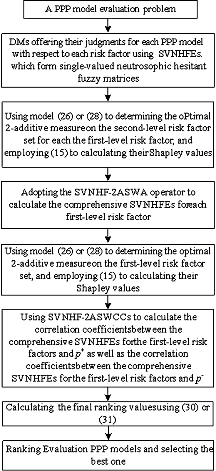
Step 8: End.
To show the procedure of the above algorithm clearly, please see Fig. 1.
6A Case Study
To show the concrete application of the offered algorithm in Section 5.2, this part offers a practical example for evaluating PPP models for the high-speed rail.
Example 1.
To promote the traffic condition, the Chinese government intends to build a high-speed railway, which spans two provinces of China with a total length of more than 600 kilometers and a planned total investment of 2 billion US dollars. Its design speed is 300 kilometers per hour. Due to the complexity of the project, the government needs to select the most suitable PPP model to complete the project according to the risk analysis. First, it needs to form an evaluation team, which includes 15 members composed by governor, mayor, railway minister, manager, sector managers, experts and scholars. To avoid interaction, they are required to provide their preferences anonymously. Because of the difference of their expertise and the complexity of the project, different preferred, indeterminacy and non-preferred judgments may be offered by different persons. To deal with this situation, SVNHFE is a good choice that can denote these three aspects using several values in
Table 4
The single-valued neutrosophic hesitant fuzzy decision matrix
Table 5
The single-valued neutrosophic hesitant fuzzy decision matrix
Table 6
The single-valued neutrosophic hesitant fuzzy decision matrix
Table 7
The single-valued neutrosophic hesitant fuzzy decision matrix
Table 8
The range of known weighting information.
| The first-level risk factor | The range of known weighting information | The second-level risk factor | The range of known weighting information |
To select the most suitable PPP model, the following procedure is needed:
Step 1: Model (28) is employed to determine the 2-additive measure on the second-level risk factor set for each first-level risk factor. Taking the second-level risk factor set for
(32)
Solving model (32) using LINGO, we obtain
Furthermore, the Shapley values are
Similarly, the Shapley values of the second-level risk factors for the first-level risk factor
Step 2: The SVNHF-2ASWA operator is used to aggregate SVNHFEs on the second-level evaluation risk factors, by which the comprehensive SVNHFEs of the thirteen PPP models for each first-level risk factor are obtained. Taking the first PPP model for
Step 3: Model (28) is again adopted to determine the optimal 2-additive measure μ on the first-level risk factor set, where the following is obtained:
(33)
Step 4: Using SVNHF-2ASWCCs to calculate correlation coefficient, which are shown in Table 9.
Step 5: According to Table 9, (30) and (31), the ranking values are obtained as follows:
Table 9
| 0.77 | 0.9 | 0.74 | 0.80 | |
| 0.96 | 0.66 | 0.86 | 0.53 | |
| 0.91 | 0.74 | 0.77 | 0.59 | |
| 0.71 | 0.82 | 0.67 | 0.69 | |
| 0.94 | 0.71 | 0.79 | 0.55 | |
| 0.76 | 0.81 | 0.72 | 0.80 | |
| 0.78 | 0.86 | 0.67 | 0.70 | |
| 0.93 | 0.65 | 0.85 | 0.58 | |
| 0.97 | 0.57 | 0.94 | 0.49 | |
| 0.79 | 0.83 | 0.72 | 0.73 | |
| 0.68 | 0.88 | 0.54 | 0.69 | |
| 0.63 | 0.92 | 0.52 | 0.76 | |
| 0.94 | 0.63 | 0.85 | 0.57 |
Step 6: According to the ranking values obtained in Step 5, we derive the below rankings
Table 10
Ranking results based on different methods.
| Geometric mean based SVNHF-2ASWCC | Maximum based SVNHF-2ASWCC | Şahin and Liu’s correlation coefficient (Şahin and Liu, 2017) | |
| Ranking values of | 0.461 | 0.481 | 0.617 |
| Ranking values of | 0.593 | 0.619 | 0.875 |
| Ranking values of | 0.553 | 0.567 | 0.736 |
| Ranking values of | 0.464 | 0.493 | 0.594 |
| Ranking values of | 0.57 | 0.59 | 0.826 |
| Ranking values of | 0.484 | 0.475 | 0.651 |
| Ranking values of | 0.476 | 0.489 | 0.639 |
| Ranking values of | 0.59 | 0.596 | 0.804 |
| Ranking values of | 0.63 | 0.657 | 0.892 |
| Ranking values of | 0.488 | 0.494 | 0.658 |
| Ranking values of | 0.436 | 0.439 | 0.509 |
| Ranking values of | 0.408 | 0.407 | 0.468 |
| Ranking values of | 0.6 | 0.6 | 0.834 |
| Ranking using geometric mean based SVNHF-2ASWCC | |||
| Ranking using maximum based SVNHF-2ASWCC | |||
| Ranking using Şahin and Liu’s correlation coefficient | |||
In this example, when Şahin and Liu’s method (Şahin and Liu, 2017) is applied, the final ranking values are obtained as follows:
Table 10 shows that different rankings are obtained based on different correlation coefficients. However, all of them show that the PPP model
This example shows that different rankings may be obtained using different correlation coefficients. This is because their principles are different. The geometric mean based SVNHF-2ASWCC adopts the geometric mean of associated items to calculate correlation coefficient, and the maximum based SVNHF-2ASWCC uses the maximum of associated items to calculate correlation coefficient. Just as the above analysis, we suggest the pessimistic DMs to use maximum based SVNHF-2ASWCC and the optimistic DMs to employ geometric mean based SVNHF-2ASWCC. As for Şahin and Liu’s correlation coefficient, it needs to add extra values into SVNHFEs and calculate correlation coefficient based on the corresponding ordered values. Furthermore, new correlation coefficients employ the 2-additive Shapley values as the weights of risk factors that can reflect the interactions among their importance. Meanwhile Şahin and Liu’s correlation coefficient is based on the assumption that there is no interaction among the weights of risk factors and it uses additive measures.
To show the differences between new method and Şahin and Liu’s method in view of their principles intuitively, please see Table 11.
Table 11
The comparison between two calculate correlation based decision making methods.
| Methods | Does it change the original decision making information? | Does it need the length of the compared SVNHFSs to be equal? | Does it consider the situation where the weighting information is incompletely known? | Can it deal with the case where there are interactive characteristics? |
| Şahin and Liu’s method (Şahin and Liu, 2017) | YES | YES | NO | NO |
| New method | NO | NO | YES | YES |
7Conclusions
There is an increasing popularity of PPP applications in infrastructure development. When PPP brings good opportunities for efficient public service and management, there are usually many types of risks due to different cultural, political, economic, and environmental problems. To minimize the risk of PPP application, it is imperative to find a suitable and comprehensive decision making method. To do this, this paper first analyses several types of PPP models and constructs a decision making index system by considering the risk factors. Then, SVNHFSs are applied to deal with uncertainties in the evaluation of PPP models. After that, two new correlation coefficients of SVNHFSs based on 2-additive measure and the Shapley function are introduced that can cope with the situation where elements in a set are interactive. Furthermore, a new algorithm is provided to evaluate PPP models. Finally, a case study is selected to demonstrate the feasibility and efficiency of this new algorithm. Compared with other methods, the main drawback of the new method seems to be more complicated when calculating the 2-additive Shapley value. However, with the help of software and the computer technology, this problem can be easily addressed. It is worth noting that we can follow new correlation coefficients for SVNHFSs to similarly study single-valued neutrosophic hesitant fuzzy distance measure and single-valued neutrosophic hesitant fuzzy similarity measure.
In the future, we will continue to research the theory of decision making with single-valued neutrosophic hesitant fuzzy information. In terms of application, we only research the application of SVNHFSs in evaluating PPP models for the high-speed rail. Similarly, we can apply the new method in some other fields, such as project management (Mohamed and Mccoan, 2001), real estate investment (Ginevicius and Zubrecovas, 2009), ecological environment management (Huang et al., 2003), information system (Gudas and Lopata, 2016; Ai et al., 2016), and supply chain management (Brandenburg et al., 2014). In some cases, some judgments may be missing due to various reasons. Therefore, we shall explore multi-attribute decision making with incomplete information (Ureña et al., 2015; Capuano et al., 2018). Furthermore, we shall continue to research decision making methods with other types of fuzzy sets such as interval neutrosophic hesitant fuzzy sets (Ye, 2016) and interval neutrosophic linguistic sets (Ye, 2014a).
References
1 | Ai, S.Z., Du, R., Brugha, C.M., Wang, H.P. ((2016) ). Pointing to priorities for multiple criteria decision making – the case of a MIS-based project in China. International Journal of Information Technology & Decision Making, 15: (3), 683–702. |
2 | Ahmadabadi A.A., Heravi, G. ((2019) ). Risk assessment framework of PPP-megaprojects focusing on risk interaction and project success. Transportation Research Part A: Policy and Practice, 124: , 169–188. |
3 | Akansha, M., Amit, K. ((2019) ). Commentary on “New aggregation operators of single-valued neutrosophic hesitant fuzzy set and their application in multi-attribute decision making”. Pattern Analysis and Applications, 22: (3), 1207–1209. |
4 | Akintoye, A., Hardcastle, C., Beck, M., Chinyio, E., Darinka Asenova, D. ((2003) ). Achieving best value in private finance initiative project procurement. Construction Management and Economics, 21: (5), 461–470. |
5 | An, X.W., Wang, Z.F., Li, H.M., Ding, J.Y. ((2018) ). Project delivery system selection with interval-valued intuitionistic fuzzy set group decision-making method. Group Decision and Negotiation, 27: (4), 689–707. |
6 | Atanassov, K.T. ((1986) ). Intuitionistic fuzzy sets. Fuzzy Sets and Systems, 20: (1), 87–96. |
7 | Bao, F.Y., Martek, I., Chen, C., Chan, A.P., Yu, Y. ((2018) ). Lifecycle performance measurement of public-private partnerships: a case study in China’s water sector. International Journal of Strategic Property Management, 22: (6), 516–531. |
8 | Biswas, P., Pramanik, S., Giri, B.C. ((2016) a). Some distance measures of single valued neutrosophic hesitant fuzzy sets and their applications to multiple attribute decision making. In: New Trends in Neutrosophic Theory and Applications, pp. 27–34. |
9 | Biswas, P., Pramanik, S., Giri, B.C. ((2016) b). GRA method of multiple attribute decision making with single valued neutrosophic hesitant fuzzy set information. In: New Trends in Neutrosophic Theory and Applications, pp. 55–63. |
10 | Brandenburg, M., Govindan, K., Sarkis, J., Seuring, S. ((2014) ). Quantitative models for sustainable supply chain management: developments and directions. European Journal of Operational Research, 233: , 299–312. |
11 | Budayan, C. ((2018) ). Evaluation of delay causes for BOT projects based on perceptions of different stakeholders in Turkey. Journal of Management in Engineering, 35: (1), 1–13. |
12 | Capuano, N., Chiclana, F., Fujita, H., Herrera-Viedma, E., Loia, V. ((2018) ). Fuzzy group decision making with incomplete information guided by social influence. IEEE Transactions on Fuzzy Systems, 26: (3), 1704–1718. |
13 | Chen, Y.Q., Lu, H.Q., Lu, W.X., Zhang, N. ((2010) ). Analysis of project delivery systems in Chinese construction industry with data envelopment analysis (DEA). Engineering, Construction and Architectural Management, 17: (6), 598–614. |
14 | Chen, N., Xu, Z.S., Xia, M.M. ((2013) ). Correlation coefficients of hesitant fuzzy sets and their applications to clustering analysis. Applied Mathematical Modelling, 37: , 2197–2211. |
15 | Dai, Q.T., Molenaar, K.R. ((2015) ). Risk-based project delivery selection model for highway design and construction. Journal of Construction Engineering and Management, 141: (12), 1–9. |
16 | Delmon, J. ((2000) ). BOO/BOT projects: a commercial and contractual guide. Sweet and Maxwell, 1: (1), 40–62. |
17 | Feng, K., Wang, S.Q., Li, N., Wu, C.L., Xiong, W. ((2018) ). Balancing public and private interests through optimization of concession agreement design for user-pay PPP projects. Journal of Civil Engineering and Management, 24: (2), 116–129. |
18 | Ghavamifar, K., Touran, A. ((2008) ). Alternative project delivery systems: applications and legal limits in transportation projects. Journal of Professional Issues in Engineering Education and Practice, 134: (1), 106–111. |
19 | Ginevicius, R., Zubrecovas, V. ((2009) ). Selection of the optimal real estate investment project basing on multiple criteria evaluation using stochastic dimensions. Journal of Business Economics and Management, 10: , 261–270. |
20 | Grabisch, M. ((1997) ). K-order additive discrete fuzzy measures and their representation. Fuzzy Sets and Systems, 92: (2), 167–189. |
21 | Gudas, S., Lopata, A. ((2016) ). Towards internal modelling of the information systems application domain. Informatica, 27: (1), 1–29. |
22 | Huang, Y.W. (2007). Research on evaluation method and decision making of PPP project. Shanghai, Tongji University, pp. 8-11. |
23 | Huang, L., Tan, Y., Song, X., Huang, X., Wang, H., Zhang, S., Dong, J., Chen, R. ((2003) ). The status of the ecological environment and a proposed protection strategy in Sanya Bay, Hainan Island, China. Marine Pollution Bulletin, 47: (1–6), 180–186. |
24 | Jang, S. (2011). A concessionaire selection decision model development and application for the PPP project procurement. University of Southampton, School of Management, Doctoral Thesis. |
25 | Jin, H.Y., Liu, S.J., Liu, C.L., Udawatta, N. ((2019) ). Optimizing the concession period of PPP projects for fair allocation of financial risk. Engineering Construction and Architectural Management, 26: (10), 2347–2363. |
26 | John, E.S., Isr, W. ((2003) ). Alternate financing strategies for build-operate-transfer projects. Journal of Construction Engineering and Management, 129: (2), 205–213. |
27 | Ke, Y.J., Wang, S.Q., Chan, A.P.C., Lam, P.T.I. ((2010) ). Preferred risk allocation in China’s public-private partnership (PPP) projects. International Journal of Project Management, 28: (5), 482–492. |
28 | Kwofie, T.E., Aigbavboa, C.O., Thwala, W.D. ((2019) ). Communication performance challenges in PPP projects: cases of Ghana and South Africa. Built Environment Project and Asset Management, 9: (5), 628–641. |
29 | Li, X., Zhang, X.H. ((2018) ). Single-valued neutrosophic hesitant fuzzy Choquet aggregation operators for multi-attribute decision making. Symmetry, 10: , 1–15. 2018. |
30 | Liu, C.F., Luo, Y.S. ((2019) ). New aggregation operators of single-valued neutrosophic hesitant fuzzy set and their application in multi-attribute decision making. Pattern Analysis and Applications, 22: (2), 417–427. |
31 | Liu, Y., Xu, Y.L., Wang, Z.Y. ((2018) a). The effect of public target on the public-private partnership (PPP) residential development. International Journal of Strategic Property Management, 22: (5), 415–423. |
32 | Liu, S.J., Jin, H.Y., Xie, B.Z., Liu, C.L., Mills, A. ((2018) b). Concession period determination for PPP retirement village. International Journal of Strategic Property Management, 22: (5), 424–435. |
33 | Liu, B., Shen, J.Q., Meng, Z.J., Sun, F.H. ((2018) c). A survey on the establishment and application of social capital partner selection system for the new profit PPP project. KSCE Journal of Civil Engineering, 22: (10), 3726–3737. |
34 | Luu, D.T., Ng, S.T., Chen, S.E. ((2005) ). Formulating procurement selection criteria through case-based reasoning approach. Journal of Computing in Civil Engineering, 19: (3), 269–276. |
35 | Mahdi, I.M., Alreshaid, K. ((2005) ). Decision support system for selecting the proper project delivery method using analytical hierarchy process (AHP). International Journal of Project Management, 23: (7), 564–572. |
36 | Meng, F.Y., Tang, J. ((2013) ). Interval-valued intuitionistic fuzzy multiattribute group decision making based on cross entropy measure and Choquet integral. International Journal of Intelligent Systems, 28: (12), 1172–1195. |
37 | Meng, F.Y., Chen, X.H. ((2015) a). Interval-valued intuitionistic fuzzy multi-criteria group decision making based on cross entropy and 2-additive measures. Soft Computing, 19: (7), 2071–2082. |
38 | Meng, F.Y., Chen, X.H. ((2015) b). Correlation coefficients of hesitant fuzzy sets and their application based on fuzzy measures. Cognitive Computation, 7: (4), 445–463. |
39 | Meng, F.Y., Tang, J., Li, C.L. ((2018) ). Uncertain linguistic hesitant fuzzy sets and their application in multi-attribute decision making. International Journal of Intelligent Systems, 33: (3), 586–614. |
40 | Mohamed, S., Mccoan, A.K. ((2001) ). Modelling project investment decisions under uncertainty using possibility theory. International Journal of Project Management, 19: (4), 231–241. |
41 | Murthy, C.A., Pal, S.K., Majumder, D.D. ((1985) ). Correlation between two fuzzy membership functions. Fuzzy Sets and Systems, 17: (1), 23–38. |
42 | Ogunlana, S.O. ((1997) ). Build operate transfer procurement traps: examples from transportation projects in Thailand. In: Proceedings of the CIB W92 Symposium on Procurement. IF Research Corporation, pp. 585–594. |
43 | Osei-Kyei, R., Chan, A.P.C. ((2018) a). Stakeholders’ perspectives on the success criteria for public-private partnership projects. International Journal of Strategic Property Management, 22: (2), 131–142. |
44 | Osei-Kyei, R., Chan, A.P.C. ((2018) b). Comparative study of governments’ reasons/motivations for adopting Public-Private Partnership Policy in developing and developed economies/countries. International Journal of Strategic Property Management, 22: (5), 403–414. |
45 | Osei-Kyei, R., Chan, A.P., Javed, A.A., Ameyaw, E.E. ((2017) ). Critical success criteria for public-private partnership projects: international experts’ opinion. International Journal of Strategic Property Management, 21: (1), 87–100. |
46 | Pang, J.J., Wang, J.Q., Hu, J.H., Tian, C. ((2018) ). Multi-criteria decision-making approach based on single-valued neutrosophic hesitant fuzzy geometric weighted choquet integral heronian mean operator. Journal of Intelligent & Fuzzy Systems, 33: (3), 3661–3674. |
47 | Pellegrino, R., Carbonara, N., Costantino, N. ((2019) ). Public guarantees for mitigating interest rate risk in PPP projects. Built Environment Project and Asset Management, 9: (2), 248–261. |
48 | Şahin, R., Liu, P.D. ((2016) ). Distance and similarity measures for multiple attribute decision making with single-valued neutrosophic hesitant fuzzy information. In: New Trends in Neutrosophic Theory and Applications, pp. 35–54. |
49 | Şahin, R., Liu, P.D. ((2017) ). Correlation coefficient of single-valued neutrosophic hesitant fuzzy sets and its applications in decision making. Neural Computing and Applications, 28: (6), 1387–1395. |
50 | Shakeri, E., Dadpour, M., Jahromi, H.A. ((2015) ). The combination of fuzzy ELECTRE and SWOT to select private sectors in partnership projects case study of water treatment project in Iran. International Journal of Civil Engineering, 13: (1A), 55–67. |
51 | Shalaby, A., Hassanein, A. ((2019) ). A decision support system (DSS) for facilitating the scenario selection process of the renegotiation of PPP contracts. Engineering Construction and Architectural Management, 26: (6), 1004–1023. |
52 | Shapley, L.S. ((1953) ). A value for n-person game. In: Kuhn, H., Tucker, A. (Eds.), Contributions to the Theory of Games. Princeton University Press, Princeton. |
53 | Smarandache, F. ((1999) ). A Unifying Field in Logics. Neutrosophy: Neutrosophic Probability, Set and Logic. American Research Press, Rehoboth. |
54 | Song, J.B., Yu, Y.Z., Jin, L.L., Feng, Z. ((2018) ). Early termination compensation under demand uncertainty in public-private partnership projects. International Journal of Strategic Property Management, 22: (6), 532–543. |
55 | Su, L.M., Wang, T.Z., Wang, L.Y., Li, H.M., Cao, Y.C. ((2019) ). Project procurement method selection using a multi-criteria decision-making method with interval neutrosophic sets. Information, 10: (6), 1–14. |
56 | Sugeno, M. (1974). Theory of Fuzzy Integral and its Applications. Doctorial Dissertation, Tokyo Institute of Technology. |
57 | Szmidt, E., Kacprzyk, J. ((2010) ). Correlation of intuitionistic fuzzy sets. In: International Conference on Information Processing and Management of Uncertainty in Knowledge-Based Systems. Springer, Berlin, Heidelberg, pp. 169–177. |
58 | Torra, V. ((2010) ). Hesitant fuzzy sets. International Journal of Intelligent Systems, 25: (6), 529–539. |
59 | Ureña, M.R., Chiclana, F., Morente-Molinera, J.A., Herrera-Viedma, E. ((2015) ). Managing incomplete preference relations in decision making: a review and future trends. Information Sciences, 302: (1), 14–32. |
60 | Valipour, A., Yahaya, N., Md Noor, N., Mardani, A., Antuchevičienè, J. ((2016) ). A new hybrid fuzzy cybernetic analytic network process model to identify shared risks in PPP projects. International Journal of Strategic Property Management, 20: (4), 409–416. |
61 | Wang, S., Qin, K.L. ((2015) ). Study on decision making of PPP project contract awarding mode based on theory of intuitionistic fuzzy sets. Yangtze River, 46: (1), 66–69. |
62 | Wang, H., Smarandache, F., Zhang, Y.Q., Sunderraman, R. ((2005) ). Interval Neutrosophic Sets and Logic: Theory and Applications in Computing. Hexis, Phoenix, Arizona, USA. |
63 | Wang, H., Smarandache, F., Zhang, Y.Q., Sunderraman, R. ((2010) ). Single valued neutrosophic sets. Multispace and Multistructure, 4: , 410–413. |
64 | Weissenböck, S., Girmscheid, G. (2013). Concept of a quantitative project selection model for PPP projects. Auf: CIB World Building Congress. |
65 | Xu, Z.S. ((2010) ). Choquet integrals of weighted intuitionistic fuzzy information. Information Sciences, 180: (5), 726–736. |
66 | Xu, D., Hong, Y., Xiang, K. ((2019) ). A method of determining multi-attribute weights based on single-valued neutrosophic numbers and its application in TODIM. Symmetry, 11: (4), 1–12. |
67 | Yan, X., Chong, H.Y., Zhou, J., Sheng, Z.H., Xu, F. ((2020) ). Fairness preference based decision-making model for concession period in PPP projects. Journal of Industrial and Management Optimization, 16: (1), 11–23. |
68 | Yang, C.L., Shieh, M.C., Huang, C.Y., Tung, C.P. ((2018) ). A derivation of factors influencing the successful integration of corporate volunteers into public flood disaster inquiry and notification systems. Sustainability, 10: (6), 1–31. 1973. |
69 | Ye, J. ((2013) ). Multicriteria decision-making method using correlation coefficient under single-valued neutrosophic environment. International Journal of General Systems, 42: (4), 386–394. |
70 | Ye, J. ((2014) a). Some aggregation operators of interval neutrosophic linguistic numbers for multiple attribute decision making. Journal of Intelligent and Fuzzy Systems, 27: (5), 2231–2241. |
71 | Ye, J. ((2014) b). Improved correlation coefficients of single valued neutrosophic sets and interval neutrosophic sets for multiple attribute decision making. Journal of Intelligent and Fuzzy Systems, 27: (5), 2453–2462. |
72 | Ye, J. ((2015) ). Multiple-attribute decision-making method under a single-valued neutrosophic hesitant fuzzy environment. Journal of Intelligent Systems, 24: (1), 23–36. |
73 | Ye, J. ((2016) ). Correlation Coefficients of interval neutrosophic hesitant fuzzy sets and its application in a multiple attribute decision making method. Informatica, 27: (1), 179–202. |
74 | Ye, J. ((2018) ). Multiple-attribute decision-making method using similarity measures of single-valued neutrosophic hesitant fuzzy sets based on least common multiple cardinality. Journal of Intelligent & Fuzzy Systems, 34: (6), 4203–4211. |
75 | Yuan, J., Skibniewski, M.J., Li, Q., Zheng, L. ((2010) ). Performance objectives selection model in public-private partnership projects based on the perspective of stakeholders. Journal of Management Engineering, 26: (1), 89–104. |
76 | Zadeh, L.A. ((1965) ). Fuzzy sets. Information Control, 8: (3), 338–353. |
77 | Zadeh, L.A. ((1975) ). The concept of a linguistic variable and its application to approximate reasoning-I. Information Sciences, 8: (3), 199–249. |
78 | Zhang, X.Q. ((2005) ). Paving the way for public-private partnerships in infrastructure development. Journal of Construction Engineering and Management, 1311: (1), 71–80. |
79 | Zhang, C.L., Liang, Y.Z., Huang, Z., Qiao, H.J., Zhang, S. ((2019) ). Selection of PPP program models based on ecological compensation in the Chishui Watershed. Water Policy, 21: (3), 582–601. |


