
Ranking comment sorting policies in online debates
Abstract
Online debates typically possess a large number of argumentative comments. Most readers who would like to see which comments are winning arguments often only read a part of the debate. Many platforms that host such debates allow for the comments to be sorted, say from the earliest to latest. How can argumentation theory be used to evaluate the effectiveness of such policies of sorting comments, in terms of the actually winning arguments displayed to a reader who may not have read the whole debate? We devise a pipeline that captures an online debate tree as a bipolar argumentation framework (BAF), which is sorted depending on the policy, giving a sequence of induced sub-BAFs representing how and how much of the debate has been read. Each sub-BAF has its own set of winning arguments, which can be quantitatively compared to the set of winning arguments of the whole BAF. We apply this pipeline to evaluate policies on Kialo debates, where it is shown that reading comments from most to least liked, on average, displays more winners than reading comments earliest first. Therefore, in Kialo, reading comments from most to least liked is on average more effective than reading from the earliest to the most recent.
1.Introduction
1.1.Background and motivations
The Internet has enabled people to share their views about many topics online, ranging from commenting on important news events11 to debating philosophical stances.22 Given that the number of Internet users grew eight-fold to over three billion worldwide between 2000 to 2016 [27], it is not surprising that such discussions have also grown both in the number of comments posted and the range of topics discussed [19]. Many online discussions now contain so many comments that it is unrealistic for a normal Internet user to read every single point being made; it is expected that a user interested in a given topic of debate would read only a fragment of the entire discussion. To help users, many online platforms that host such discussions allow for the comments to be sorted according to some policy, such as displaying the comments from the most liked to the least liked.
Further, comments exchanged over such discussions are often argumentative in nature, and can be modelled with argumentation theory (e.g. [7,31]); this can resolve disagreements arising from such online debates by finding the winning arguments based on normative yet intuitive criteria. Suppose that a user would like to know which arguments have prevailed at a given moment, but does not have time to read every comment. Such a reader may think that a given argument has won when it has been rebutted by further comments which have not yet been read. The goal of this paper is to compare how various comment sorting policies can affect the number of actually winning arguments exposed to a reader, depending on how much of the debate has been read. A precise way to compare such policies will bring visibility to which arguments should win, thus helping readers to better navigate and understand large and argumentative online debates (e.g. [1,8,14,28,32,36]).
1.2.Overview of contributions
We apply argumentation theory, data mining and statistics to build a pipeline that compares comment sorting policies by measuring the number of actually winning arguments each policy displays to a reader who has only read a part of the debate. Intuitively, we mine online debates (e.g. such as [13,17,35]), and represent them as directed graphs (digraphs), whose nodes are the comments made during the debates and the edges denote which comment is replying to which other comment. As such debates begin with an initial comment, and each subsequent comment replies to exactly one other comment, these debates are trees, which is what we will restrict our analysis to in this paper, leaving other debate network topologies for future work (see Section 6).
Argumentation theory (e.g. [31]) is the branch of artificial intelligence concerned with the rational and transparent resolution of disagreements. Abstractly, arguments and their disagreements (called attacks) are represented as digraphs, called argumentation frameworks (AFs) [15]. However, in real debates, arguments can agree with each other as well as disagree. Subsequent theoretical developments have incorporated support between arguments, which can be interpreted as “agreement”. An AF where each directed edge is either an attack or a support is called a bipolar argumentation framework (BAF) [9,10]. There are principled ways of determining from various combinations of attacks and supports which arguments are winning. Therefore, subject to an appropriate representation of the debate one is interested in, resolving the disagreements is modelled by finding a subset of winning arguments.
To enable the application of argumentation theory, the pipeline makes two idealised assumptions: (1) each comment qualifies as a self-contained argument, and (2) each reply is either supporting or attacking. Of course, the vast majority of online debates are not so “clean”, but the pipeline does not preclude methods that allow for the identification of whether a comment qualifies as an argument (as opposed to, e.g. an insult), or whether a reply between comments is an attack or a support (e.g. [3,11]). Assuming that there is a relatively “clean” online debate, or that we can incorporate sophisticated data cleaning techniques to the pipeline, then we can treat the online debate formally as a BAF. Furthermore, if this debate is a tree, then the set of winning arguments is unique [15, Theorem 30].
To model the idea of a comment sorting policy, the pipeline linearly sorts all comments based on the direction of replies, such that if comment b replies to comment a, then a is read prior to b, while preserving the structure of each thread (see Section 3.1). However, when multiple comments
Suppose the debate has
The pipeline then aggregates the
As mentioned earlier, if for simplicity one does not wish to incorporate argument mining techniques, then these calculations can only make sense if we do have a dataset of “clean” online debates, i.e. where each comment qualifies as a self-contained argument, and each reply is classified as either an attack or a support. Fortunately, the online debating platform Kialo33 provides such a “clean” dataset, thanks to its moderation policy that ensures every comment is a concise and relevant argument to the topic being discussed that is replying either positively (supporting) or negatively (attacking) to another comment (or no such reply if it is the root comment of a discussion). We have mined Kialo data until March 2019 (see Section 4), and processed this data via our proposed pipeline. Subject to suitable aggregation and identification of what “likes” and “time” mean for each comment (see Section 5.2), the pipeline shows that reading Kialo debates from the most to least “liked” comment displays more actually winning arguments, on average, than reading Kialo debates from the earliest comment to the most recent comment. We close by conjecturing why this is and speculate on how robust this result is to less “clean” online debates.
1.3.Structure of this paper
In Section 2, we will summarise the relevant background in argumentation theory and related work. In Section 3, we will explain the pipeline and clarify its assumptions and limitations. In Section 4, we overview Kialo, explain how it validates the pipeline’s assumptions, explain how we have mined the data, and offer summary statistics. In Section 5, we articulate the comment sorting policies based on likes and time for Kialo, and have the pipeline measure which policy is more effective. Section 6 concludes with future work.
2.Technical background and related work
In this section we recap relevant aspects of abstract argumentation theory and bipolar argumentation theory. We then give a brief survey of argument mining and its application to online debates.
2.1.Abstract argumentation theory
From [15]: An abstract argumentation framework (AF) is a digraph
We say S is admissible iff S is both cf and sd. There are four basic notions of “winning arguments”, each of which builds on admissibility [15]. We say S is a complete extension iff S is admissible and that
2.2.Bipolar argumentation theory
Bipolar argumentation theory extends AFs with a support relation [9]. A bipolar argumentation framework (BAF) is a structure
There are principled ways to absorb
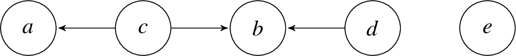
Example 2.2
Example 2.2(Example 2.1 continued).
Figure 2 illustrates the BAF where
Fig. 2.
The BAF from Example 2.2, where green (dotted) edges denote supports and red (solid) edges denote attacks.
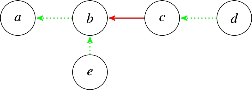
The support paths of length 1 in this BAF are
2.3.Argument mining and the analysis of online debates
Argument mining (e.g. [23,24]) seeks to identify and extract structured, self-contained arguments and inter-argument relationships from natural language text to (amongst many other applications) resolve conflicting points of view expressed in online debates (e.g. [6,7]). However, in order to successfully apply argumentation theory to real data, one would need a relatively “clean” dataset of online debates. This is non-trivial, because most online debates are very “noisy”. For example, Twitter Tweets are often too short to be treated as self-contained arguments so a preprocessing step is required to determine whether Tweets can be treated as such [3]. Further, one must formally represent the relationships between the mined arguments. In the context of applying BAFs to model online debates, we are interested in classifying whether a reply from comment a to comment b (assuming both a and b can be treated as arguments) is attacking or supporting. Existing techniques include textual entailment, which infers relevance and contradiction between pieces of natural language (e.g. [2,12]) and hence identify attacks between comments. Another way of identifying attack or support can be to calculate affective or emotional scores from key words in the comments using Linguistic Inquiry and Word Count [29,34], such that replies between comments with very similar such scores can be related to supports. A more sophisticated method for identifying attacks and supports involves deep learning [11]. Therefore, there are many argument mining techniques at our disposal if one wishes to investigate a “noisy” online debate dataset, where it cannot be assumed that each comment made by users constitutes a well-defined argument, or that every reply is either an attack or a support. We envisage that such techniques are used to first render the “noisy” online debate “clean”, then one can use the usual methods in identifying the winning set(s) of arguments.
In the next section, we will apply ideas from argumentation theory to articulate a pipeline that allows one to rank the effectiveness of various comment sorting policies in online debates, assuming that the input data is already “clean”, either because it is “naturally clean”, or that it has been “cleaned up” by techniques such as those just mentioned. Therefore, the pipeline does not preclude the use of such techniques. We will outline how such techniques can be integrated into this pipeline in Section 6.
3.A pipeline to evaluate comment sorting policies
In this section, we articulate the pipeline, based in argumentation theory, that can evaluate how best to sort comments for readers who may not have read the entire debate.
3.1.The stages of the pipeline
The pipeline consists of the following stages, where the first two stages involve validating our assumptions on the data.
(1) We input to the pipeline an online debate. The nodes are comments made in the debate that possess some attributes, e.g. upvotes, downvotes, Retweets (in the case of Twitter), time of posting, the author’s username… etc. The edges are replies, such that for comments a and b, the edge points from b to a iff b replies to a. As the online debates we will focus on in this work are trees, we will restrict to the case of trees as inputs to the pipeline, i.e. that each comment beyond the first can only reply to one other comment, and the digraph is weakly connected. Further, we do not consider time-evolution of debates, i.e. the debate accepted by the pipeline is a snapshot of the comments at that given point in time.
(2) We make the assumption that the digraph is “clean”, in that every comment can be seen as a self-contained argument, and every reply is either an attack or a support. Therefore, the debate digraph is a BAF
(3) We calculate the grounded extension,
(4) We now explain what we mean by comment sorting policy with respect to a given (numerical) attribute, and provide some simple examples; examples based on real data will be motivated and defined in Section 5.2. Our input BAF is a tree of debate comments and replies. There are many ways to read a debate. The pipeline currently considers the following way: start with the root comment, and at a given comment, read the unread reply with the most or least of that numerical attribute, until a comment with no replies has been reached (a leaf node), and then backtrack to the most recent comment where there is more than one reply, and continue. This is depth-first search (DFS), and sorts the comments in A into a list
Why is this method of reading comments plausible? We assume that a reader who is interested in the debate would start with the opening argument and read sequentially along the replies without missing any intermediate arguments, in order to fully understand each thread of the debate. Upon reaching an argument with multiple replies, the online debate platform will rank the subsequent debate replies by the chosen attribute (e.g. number of likes), therefore the reader will start reading the debate along the path with the greatest or least values of this attribute. Indeed, this is enforced to some extent in real online discussion platforms such as comments to articles in Disqus44 or The Daily Mail (a UK newspaper).55 We now give two examples:
Example 3.1
Example 3.1(Example 2.2 continued).
This example sorts the arguments to represent reading from the earliest to the most recent following DFS. Consider the BAF from Example 2.2, where
A reader would start at the root, a, which has received only one reply, b. b in turn receives two replies, c and e. Assume that e has been posted prior to c (i.e.
From now, we make the assumption of time coherence of a debate network – that if argument b replies to argument a, then
Example 3.2
Example 3.2(Example 3.1 continued).
This example sorts the arguments to represent reading from the most liked to the least liked following DFS. Consider again the BAF in Example 2.2. Suppose further that argument c is more liked than argument e. The resulting sorting policy based on DFS and reading from most to least liked will output
(5) As shown in Examples 3.1 and 3.2, comment sorting policies order the arguments in A into a list
(6) We quantitatively compare G and
and
Example 3.3
Example 3.3(Example 3.1 continued).
Reading the BAF from Example 2.2 from the earliest to the latest comment following DFS, we obtain the reading order
Table 1
The results of applying steps (5) and (6) of the pipeline in Example 3.3
| n | Comments Read | Actual winners G | Apparent winners so far, | Jaccard coefficient, |
| 0 | ∅ | 0 | ||
| 1 | 0 | |||
| 2 | 0 | |||
| 3 | 0.2 | |||
| 4 | 0.666… | |||
| 5 | 1 |
Example 3.4
Example 3.4(Example 3.2 continued).
Reading the BAF from Example 2.2 from the most liked to the least liked comment following DFS, we obtain the reading order
Table 2
The results of applying steps (5) and (6) of the pipeline in Example 3.4
| n | Comments Read | Actual winners G | Apparent winners so far, | Jaccard coefficient, |
| 0 | ∅ | 0 | ||
| 1 | 0 | |||
| 2 | 0 | |||
| 3 | 0.333… | |||
| 4 | 0.666… | |||
| 5 | 1 |
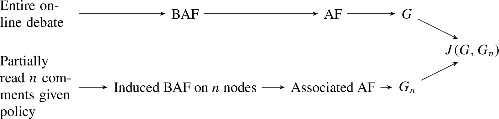
We illustrate the above six steps, for a fixed value of n, with Fig. 3 [38]:
Fig. 3.
A schematic of our pipeline used to evaluate comment sorting policies.
3.2.Formal properties of the pipeline
The following are straightforward consequences of our pipeline.
Corollary 3.5.
In our pipeline, illustrated in Fig. 3,
Proof.
If
Note that the converse to Corollary 3.5 is false, as indicated in Example 3.3 for
Corollary 3.6.
Let N be the number of arguments of our input BAF, then
Proof.
The induced BAF is the original BAF itself, hence
Intuitively, Corollary 3.5 states that if you read nothing you get nothing, and Corollary 3.6 states that if you read everything you get everything, regardless of the comment sorting policy. One further result concerns the case where all edges are supports and the policy is based on DFS.
Theorem 3.7.
Consider an input BAF
Proof.
(⇒) If
(⇐, contrapositive) Assume that there is some attacking edge
This means that in a debate where there is no disagreement, the more one reads, the more of actually winning arguments is obtained, because every additional argument read is actually winning. Further, this strictly monotonically increasing situation is only possible in the case where every reply is supporting.
3.3.How are comment sorting policies compared?
As discussed so far, the pipeline takes as input a BAF and a comment sorting policy, and returns a vector
Definition 3.8.
Given a policy P that has a
Intuitively, as the Jaccard coefficient is a measure of how many actually winning arguments the apparently winning arguments contain, having read the debate up to a certain point,
Example 3.9
Example 3.9(Examples 3.3 and 3.4 continued).
For the BAF in Example 2.2, sorting from the earliest comment to the most recent comment gives an average Jaccard of
The following corollary of Theorem 3.7 shows for the special case of debates where there is no disagreement, every policy based on DFS gives an average Jaccard of 0.5. This makes sense as we are taking the centre of mass of the diagonal line that joins
Corollary 3.10.
If the input BAF satisfies
Proof.
By Theorem 3.7, for any sorting policy based on DFS, (
3.4.Summary of the pipeline
The first contribution of this paper is a pipeline that accepts as input an online debate represented as a BAF, and a comment sorting policy, and calculates how this policy, on average, exposes the reader to the actually winning arguments, especially when the reader has not read the entire debate. We have given a running example of how the pipeline works (Examples 2.1 to 3.9).
However, the fundamental assumption of the pipeline – that a real-life online debate can be represented as a BAF – is suspect. One cannot just assume that comments posted on online debates are self-contained arguments, nor that every reply can be classified as an attack or a support. Of course, the pipeline does not preclude the use of argument mining techniques (Section 2.3) to structure online debates into a BAF for our pipeline to ingest (Section 6). In the next section, we present a dataset that we have mined, which seems to satisfy the property of being “clean”, and thus being immediately suitable for input into the pipeline as a proof of concept of how might various comment sorting policies be evaluated.
4.Kialo
We now overview Kialo, an online debating platform. We argue that its moderation policy ensures that the debates it hosts are sufficiently “clean” to be inputted into our pipeline for analysis. We summarise how the debates were mined and cleaned into BAFs for our dataset.
4.1.What is Kialo and why is Kialo “clean”?
Kialo is an online debating platform that helps people “engage in thoughtful discussion, understand different points of view, and help with collaborative decision-making.”66 In a Kialo debate, users submit claims. The starting claim is a thesis, which has at least one, but possibly more, indexing tags. Further claims then reply to existing claims, and are classified as either pro or con the claim being replied to.
Example 4.1.
Consider the Kialo discussion with thesis, “Internet companies are wrong in denying services to white supremacists.”77 One example pro argument for the thesis is, “Denying service to white supremacists might lead to extensive online censorship of non-mainstream views.” One example con argument is, “It is in the interest of Internet companies to deny services to white supremacists.”
Kialo debates are “clean” and easily-represented as BAFs without the use of argument mining tools (Section 2.3). Firstly, Kialo has a strict moderation policy, which aims to keep users engaged and promotes a well-structured discussion.88 Central to this is the enforcement of writing good claims. For example, each claim should be concise, self-contained, based on logic and facts, and make a single point that is relevant to the debate topic – in other words, claims are arguments.99 Claims should not be questions, or mere comments, or duplicated within a discussion – this excludes the possibility that claims are insults, say. Discussions are structured such that more general claims are closer to the root, and more specific claims are closer to the leaves. The conciseness of each claim allows for fine-grained support or attacks when replied to.1010 Claims that fail to meet such criteria are marked for review.1111 Either the claim is deemed unsuitable and therefore removed from the debate, or that the claim is conditionally approved after some discussion between the claim’s author and the moderators, and that the claim’s author must make satisfactory improvements for the claim to be published.1212 This validates the pipeline’s assumption that all claims made in Kialo debates can be treated as an argument.
In Kialo, every claim b that is replying to another claim a is classified by the author as pro or con a; the polarity of the reply is also suitably moderated as part of auditing the claim. Therefore, all replies are classified as either attacking or supporting. This validates our assumption that Kialo debates can be modelled as BAFs. Further, the mechanism of how claims reply to at most one other claim and that each claim is moderated to ensure that it makes a unique point mean we can assume Kialo debates are trees.
In summary, Kialo is an online debating platform. Its highly moderated nature validates our assumptions that every claim made in Kialo debates can be treated as self-contained arguments. Further, every reply between two claims in a Kialo debate must either be a support (pro) or an attack (con). Lastly, the structure of Kialo debates guarantees that the underlying digraph is a tree. It is in this sense that Kialo debates are sufficiently “clean” for us to represent them straightforwardly as BAFs without the need for further data cleaning methods.
4.2.Mining Kialo
We scraped all Kialo debates dated up until March 2019 as follows: we use the publicly visible Kialo application programming interface (API), which is used by Kialo’s front end, to acquire all the available tags used to tag individual debates; this resulted in a list of over one thousand unique tags. We then used the same API to perform a tag-based search for debates using the previously acquired list of tags. For each debate we obtained its claims, replies, and various claim attributes such as the username of the author, its text, time of posting, and votes (related to likes, see Section 5.2). This returned 1,056 debates. We then use independent means of verifying this dataset [4], which gives us a high degree of confidence that this is almost all of the debate activity on Kialo, as of March 2019.
4.3.The resulting dataset
When the debates dataset was cleaned, we noticed that some nodes (less than 1% of the total) have empty text and therefore could not be considered arguments; this is possibly due to how the data is stored in the back end of Kialo has failed to synchronise with moderators asking for a claim to be removed. Further, some reply edges violate time coherence (Section 3.1). We delete both such nodes and edges and focus on the resulting sub-discussions, on the assumption that Kialo’s moderation policy implies that sub-discussions are also self-contained, despite being separated from the thesis, due to the conciseness of each reply. This results in
5.Analysing Kialo debates with our pipeline
We now input our Kialo dataset (Section 4) into our pipeline (Section 3) and evaluate four policies.
5.1.Validating the pipeline assumptions
As stated in Section 4.1, Kialo debates are sufficiently clean such that they are readily representable as BAFs due to its design and moderation policy. Further, in our dataset, all debates are trees hence all debates (and all induced subgraphs thereof) have a well-defined set of winning arguments via the grounded extension that the pipeline calculates. This verifies Steps (1) to (3) of the pipeline (Section 3.1), apart from defining the policies to sort comments by. Lastly, we do not need to perform further natural language processing, because the BAFs are already given.
5.2.Which policies to evaluate?
To apply Step (4) of the pipeline to Kialo data, we still assume that an interested reader would read each replying comment from the root in a DFS manner as this models how the reader is getting whole conversation threads without skipping comments before backtracking to the next possible thread.
For the purposes of illustrating how the pipeline works on “cleaned” real data in this paper, we compare sorting along two attributes: likes and time; other attributes and policies will be considered in future work (Section 6), as these two attributes are readily available from Kialo data.
Time refers to the time of posting the claim, while likes is a measure of how “good” the claim is. In our dataset, each comment in a Kialo debate is already time-stamped, hence time for each comment is well-defined. However, likes is not well-defined. Conceptually, the closest attribute available in Kialo comments is the number of votes, which is a five-tuple
How can we relate the five-vector of votes v to a single number to sort claims by, which is also a proxy for likes? We use the following weighted average: define a weight vector
Example 5.1.
If a claim has
Notice if
We now define the following two w’s to form two “sort by likes” policies. Informally, the first w is a priori and the second is data-driven. Suppose we interpret these five impact categories in terms of a rational reader’s degrees of belief about the truth of the claim (e.g. [21]), so
Example 5.2.
If a claim has
One criticism of rational likes is that this idea of equal weight increases across the five impact categories is unjustified in that it assumes all readers interpret these impact categories rationally. Another approach is to weigh each impact category according to the number of votes each has received across all
Example 5.3.
If a claim has
Therefore, we enhance all nodes in each BAF of our dataset with rational and empirical likes, based on their votes vector. We define the following four policies to evaluate with our pipeline (Section 3.1):
(1) Policy 1: Non-DFS Ascending Time sorts the comments from oldest (smallest Unix time) to most recent (largest Unix time). This is “Non-DFS” because we do not follow DFS as described in Section 3.1 to serve as a baseline for the next policy; not following DFS means that a reader may move between discussion threads rather than finishing a complete thread first.
(2) Policy 2: Ascending time with DFS always choose the lowest value of (Unix) time that has not yet been chosen in DFS when there is a choice of replies – this is well-defined as there are no ties in the timestamp of comments. This displays the comments from the earliest posted to the most recently posted while preserving each branch of the debate.
(3) Policy 3: Descending rational likes with DFS, i.e. always choose the highest value of rational likes that has not yet been chosen in DFS. This sorts the comments from most to least liked following the debate branch. If there are ties, we break the tie with respect to ascending time, i.e. when choosing between two equally rationally liked comments, choose the earlier one first.
(4) Policy 4: Descending empirical likes with DFS is analogous to Policy 3, but replaces rational likes with empirical likes, with the same tie-breaking mechanism.
5.3.Results
We now measure the effectiveness of the above four policies as described in Steps (5) and (6) of Section 3.1. For each debate in our dataset, we calculate and plot
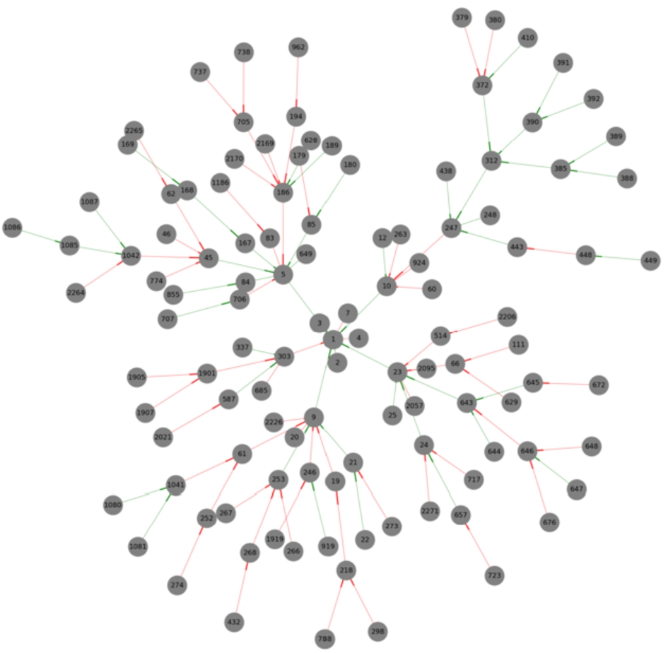
Example 5.4
Example 5.4(Example 4.2 continued).
The data cleaning process has assigned the index 2,768 to this debate. As n increases from 0 to N, Fig. 5 displays how
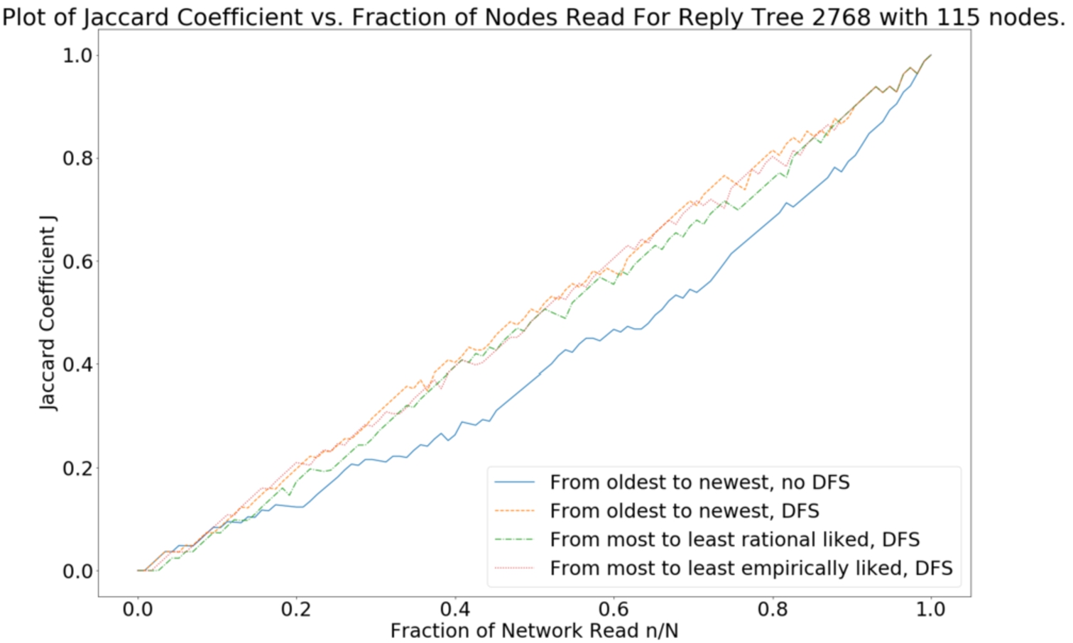
Visually, it is difficult to judge how each policy differs as all cluster around the diagonal. For each debate, we plot the detrended Jaccard,
Example 5.5
Example 5.5(Example 5.4 continued).
Figure 6 plots the detrended Jaccard vs.
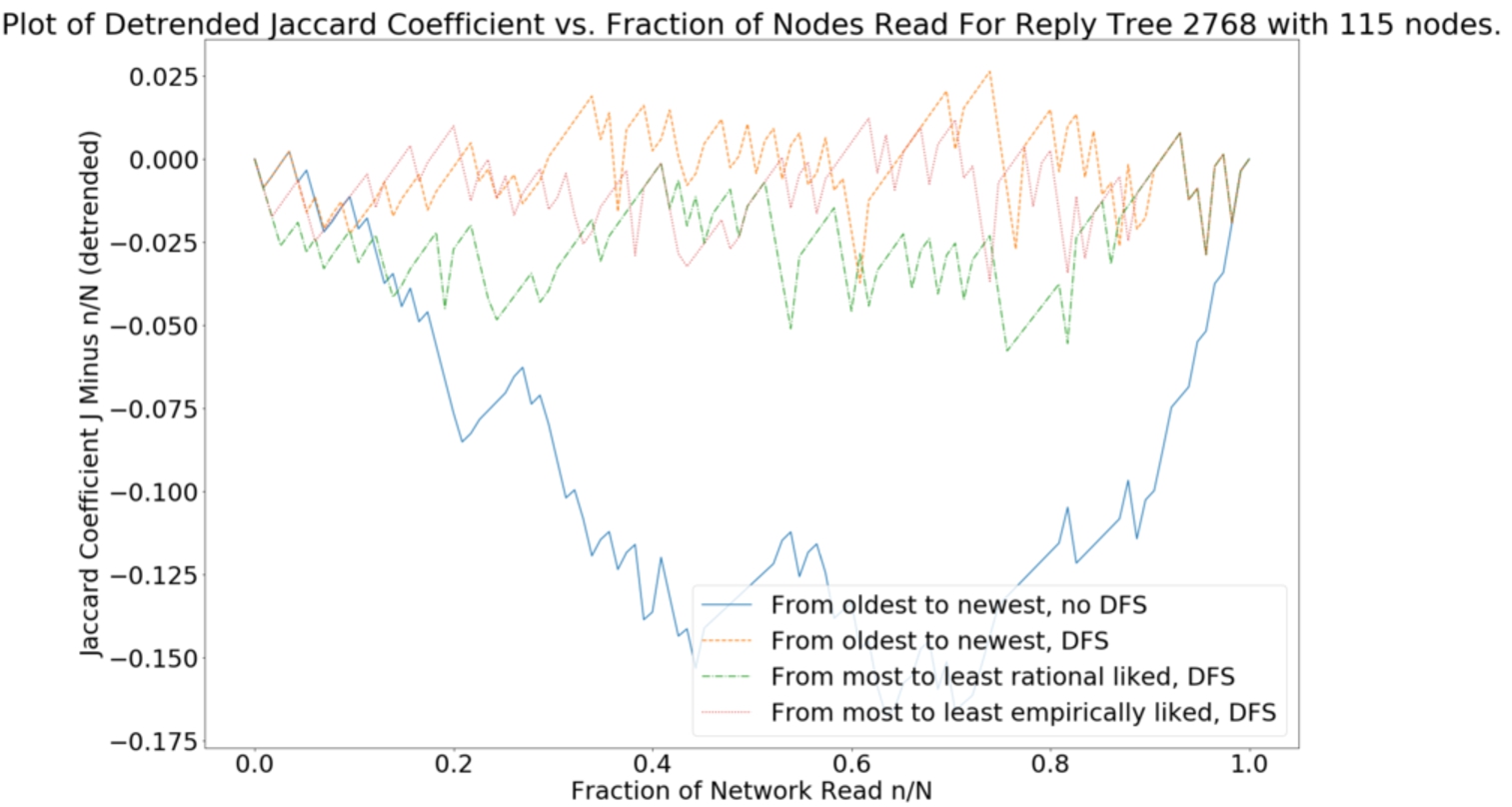
Visually, all policies are the same when reading up to
The conclusions we have drawn so far only apply to debate 2,768 (Examples 4.2 to 5.5). We are now interested in using our entire dataset of 4,365 BAFs to determine which of our four policies – Policies 1 and 2 are based on time (with or without DFS) and Policies 3 and 4 are based on likes (rational and empirical, with DFS) – is the most effective, i.e. maximises
5.4.For Kialo, sorting by likes is, on average, better than sorting by time
We repeat the calculation in Example 5.5 for all 4,365 BAFs in our dataset. Each version of Fig. 6 for each BAF will have some pattern of fluctuations about the horizontal for each policy. Instead of describing these fluctuations directly, we evaluate the policies over our dataset of debates in two ways: (1) across the entire range of
Fig. 7.
The
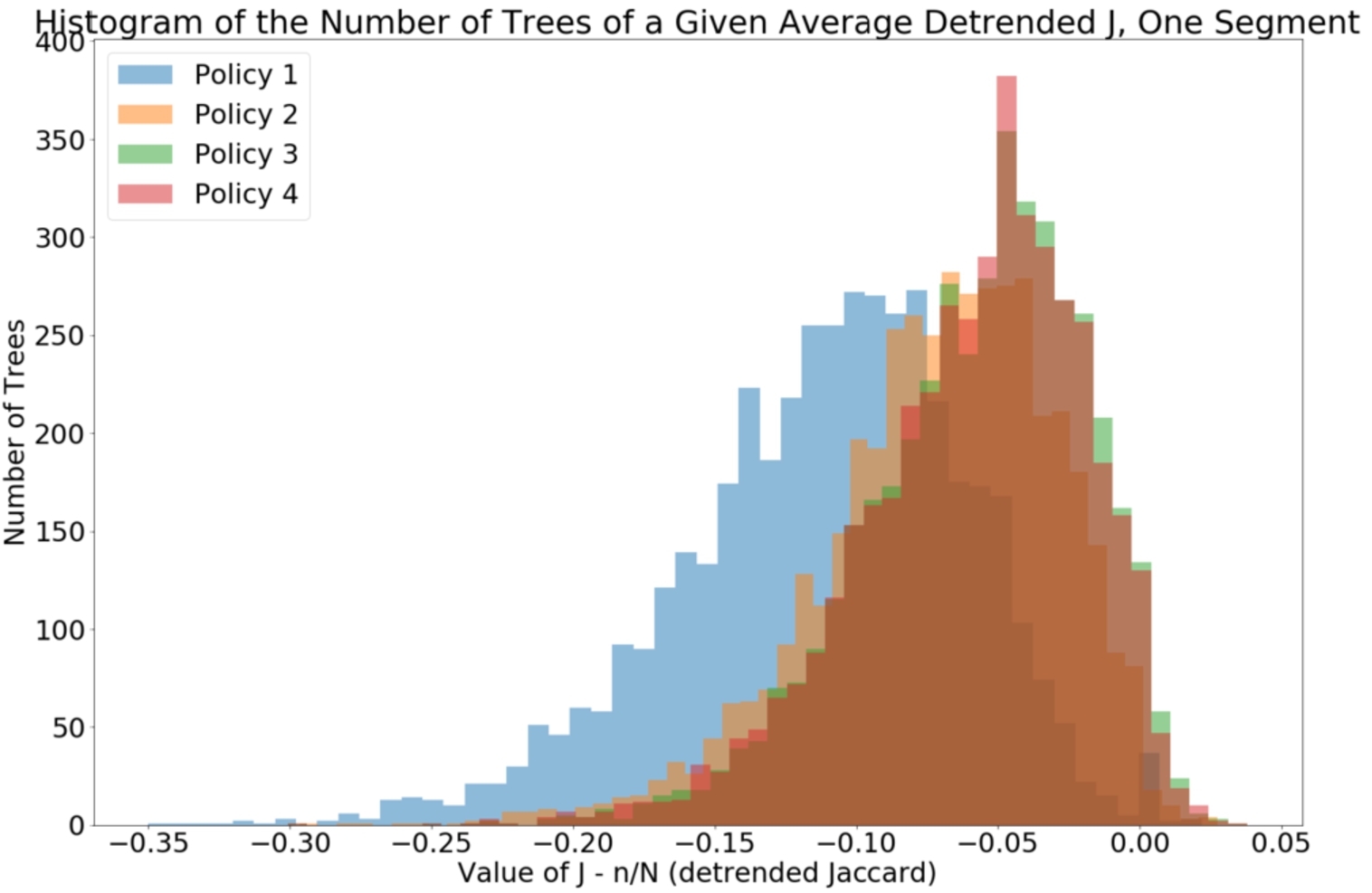
Fig. 8.
The distribution of the values of

Visually, we can see that Policy 1 is the worst policy to sort by, according to its averaged
Table 3
The summary statistics for the data behind Fig. 7
| Policy | Attribute | Direction | DFS? | Median | Mean | SSD | Minimum | Maximum |
| 1 | Time | Ascending | No | 0.051 | 0.022 | |||
| 2 | Time | Ascending | Yes | 0.042 | 0.027 | |||
| 3 | Rational Likes | Descending | Yes | 0.040 | 0.038 | |||
| 4 | Empirical Likes | Descending | Yes | 0.040 | 0.038 |
We can see that comparing the medians and means of the four policies does support that sorting by likes is better than sorting by time, and further, that time with DFS is better than time without DFS. Let us make this even more precise with an appropriate statistical test. Figure 7 displays skewed distributions, therefore we should make no assumptions on the underlying population distribution for average
As this is a non-parametric situation, we apply the Mann–Whitney test [25] to compare whether the observed distributions of average
Table 4
The results of performing a Mann–Whitney test on the dataset behind Fig. 7, in order to answer the question, “When comparing the four histograms of each policy pairwise, are they sampled from different distributions?” This is answered in the last column of the table, at a significance level of 0.05
| Sample 1 policy | Sample 2 policy | Test statistic | p-value | Significant w.r.t. |
| 1 | 2 | 5031068.5 | 0.0 | Yes |
| 1 | 3 | 3762044.0 | 0.0 | Yes |
| 1 | 4 | 3848325.5 | 0.0 | Yes |
| 2 | 3 | 7756407.5 | Yes | |
| 2 | 4 | 7875127.5 | Yes | |
| 3 | 4 | 9397703.0 | 0.137 | No |
For Fig. 7, Policy 2 beats Policy 1 (average
We now perform the same calculation for the case where instead of averaging
The summary statistics of the distributions of
Table 5
The summary statistics for the data behind Fig. 8
| Policy | Attribute | Direction | DFS? | Median | Mean | SSD | Minimum | Maximum |
| 1 | Time | Ascending | No | 0.150 | 0.172 | 0.131 | 0 | 0.571 |
| 2 | Time | Ascending | Yes | 0.188 | 0.203 | 0.128 | 0 | 0.600 |
| 3 | Rational Likes | Descending | Yes | 0.200 | 0.220 | 0.134 | 0 | 0.625 |
| 4 | Empirical Likes | Descending | Yes | 0.200 | 0.219 | 0.133 | 0 | 0.625 |
When comparing medians, Policy 1 is again the least effective. Policy 2 is more effective than Policy 1 (i.e. sorting by time with DFS is better than without DFS). Both Policies 3 and 4 are more effective than Policy 2, and they seem as effective as each other. Again, we can make this precise with the same statistical tests, hypotheses and significance levels as for the summary statistics in Fig. 7 (see Table 6).
Table 6
The results of performing a Mann–Whitney test on the dataset behind Fig. 8, in order to answer the question, “When comparing the four histograms of each policy pairwise, are they sampled from different distributions?” This is answered in the last column of the table, at a significance level of 0.05
| Sample 1 policy | Sample 2 policy | Test statistic | p-value | Significant w.r.t. |
| 1 | 2 | −12.03984 | Yes | |
| 1 | 3 | −16.97377 | Yes | |
| 1 | 4 | −16.87197 | Yes | |
| 2 | 3 | −5.460176 | Yes | |
| 2 | 4 | −5.309276 | Yes | |
| 3 | 4 | −0.175989 | 0.430 | No |
We conclude that the ordinal ranking the four policies by
6.Discussion and future work
Modern online debates are often so large in scale that the majority of Internet users cannot read all comments made. Many platforms that host these networks make use of comment sorting policies that can display the most suitable comments to readers who may not have read everything. We are interested in applying argumentation theory to measure how effective these policies are in displaying the actually winning arguments to readers who may not have read the entire network.
Our first contribution (Section 3) is a pipeline that takes as input sufficiently “clean” debates represented as bipolar argumentation trees, each having a unique set of (normatively) winning arguments. A sorting policy specifies the order to display the arguments. At each incomplete reading of the pipeline with respect to a policy, which has its own set of provisionally winning arguments from the induced sub-framework, we measure how many actually winning arguments are present using the Jaccard coefficient.
Our second contribution (Sections 4 and 5) is an application of this pipeline to Kialo debates. We argue that Kialo debates are “clean” thanks to its moderation policy. Therefore, each debate is readily-represented as a bipolar argumentation tree. The pipeline calculates, for each debate and policy, its sequence of Jaccard coefficients, one per amount of the debate read. We then aggregate these coefficients to measure how effective the policy is across all debates. As a starting point we have opted to compare policies based on sorting by likes and time, as these are the most obvious attributes available from Kialo. We find that policies that sort the comments from most to least likes are on average more effective at displaying the actually winning arguments than sorting comments from the earliest to the most recent.
This work uses Kialo as a case study on how we can apply argumentation theory to measure the effectiveness of comment sorting policies, taking advantage of Kialo’s “clean” nature. But the pipeline is agnostic to the kinds of debates and policies. In future work, we seek to determine how robust our observation that “sorting by likes is better than sorting by time” for other debates. As stated in Section 3, we cannot assume that other debates are as “clean” as Kialo, so we seek to integrate some argument mining techniques (e.g. [20], or those summarised in Section 2.3) as a pre-processing step. For example, in BBC News’ Have Your Say, the entire news article is the root argument, and the comments replying to it may not be arguments. But instead of being a star graph, some comments may mention a username or quote from another comment as a reply. Therefore, one argument mining task would be to infer replies via the text, rather than having the replies already structured like in Kialo. Another argument mining task is to infer the argumentative structure within the news article, which will then split the news article from a single root into a cluster of arguments, and one can identify the specific portions of the news text a given comment is replying to. Further, we can also investigate the time-evolution of such debates, e.g. by taking a time-ordered sequence of debate snapshots and comparing the pipeline outputs at each step.
We anticipate that for noisier datasets we may have to deal with trolls and bots that respectively make abusive comments or distribute spam (e.g. [5,18,30]). For such networks, it may be problematic to allow for the unrebutted comments to win by default, as they are the furthest away from the root and may be irrelevant or insulting. We have made an attempt at mitigating the effects of the leaf nodes winning by default [4], but other ideas involve changing the debate graph topology to have some leaves be symmetrically attacked. However, the resulting loss of a tree structure may mean our actually winning set of arguments can be non-unique, so which actually winning set of arguments (e.g. preferred or grounded) should we compare against? Or would different sorting policies guide readers to different sets of winners?
We can also consider other sorting policies. For example, in Daily Mail comments, the likes attribute contains both an upvote and a downvote. We may (e.g.) compare sorting by descending upvote with sorting by ascending downvote. As mentioned in Section 3, Daily Mail depth-2 comments are hidden under a “See all Replies” button. How does selectively revealing such comments affect the visibility of the actually winning arguments and hence the effectiveness of a policy? The four policies we have studied are chosen because they are present in most debates (Section 3), but Kialo’s user interface (UI) also displays breadth-first search, so we can investigate how effective Kialo’s UI is as a “policy”.
As for post-processing, we have alluded to the many ways the sequence of Jaccard coefficients can be aggregated in Section 5.4. We can test the robustness of our observations by considering more fine-grained averages such as averaging over e.g. the first third of
Finally, we seek to answer the question of why should sorting by likes be better than sorting by time. We hypothesise that likes is somehow related to how “good” a point that comment is making, which by standards of civil discourse raises its probability of winning and force of argument. Future work will make these notions precise.
Notes
1 E.g. BBC News – https://www.bbc.co.uk/news/uk-politics-38996179, last accessed 26/8/2020.
2 E.g. an online debate from Kialo – https://www.kialo.com/the-existence-of-god-2629, last accessed 26/8/2020.
3 https://www.kialo.com/, last accessed 26/8/2020.
4 E.g. see https://www.quantamagazine.org/physicists-debate-hawkings-idea-that-the-universe-had-no-beginning-20190606, last accessed 26/8/2020. Disqus has appropriately indented comments in the user-inteface (UI) to denote the depth of each comment within the debate tree, and sorting the comments from e.g. most to least liked follows this DFS display pattern.
5 E.g. see https://www.dailymail.co.uk/news/article-6894539/Meghan-Markle-snubs-Queens-doctors-birth-doesnt-want-men-suits.html, last accessed 26/8/2020. In contrast, the comments, although sortable by DFS, only allows replies of depth 2 (i.e. replies to the news article, and replies to replies), and displays only the first two comments amongst the depth-2 replies by default.
6 Quoted from https://www.kialo.com/about, last accessed 26/8/2020.
7 https://www.kialo.com/free-speech-on-the-internet-should-internet-companies-deny-service-to-white-supremacists-2867, last accessed 26/8/2020.
8 See https://support.kialo.com/hc/en-us/articles/360000631852-Moderating-Discussions, last accessed 26/8/2020.
9 See https://support.kialo.com/hc/en-us/articles/115000762032-Writing-Good-Claims and https://support.kialo.com/hc/en-us/articles/115000761972-Top-Tips, both accessed 23/5/2020.
10 See https://support.kialo.com/hc/en-us/articles/115001599851-Structuring-a-Discussion, last accessed 26/8/2020.
11 See https://support.kialo.com/hc/en-us/articles/115003792505, last accessed 26/8/2020.
12 Refer to the URL in Footnote 8.
13 The anonymised BAF graphs from the Kialo data would be shared upon reasonable request for research and reproducibility.
14 See https://support.kialo.com/hc/en-us/articles/115001605352-Using-Voting, last accessed 26/8/2020.
15 See https://support.kialo.com/hc/en-us/articles/115000705652-What-is-Voting-, last accessed 26/8/2020.
Acknowledgements
The authors would like to thank the three anonymous reviewers whose suggestions have greatly improved the paper. APY and NS acknowledge funding from the Space for Sharing (S4S) project (Grant No. ES/M00354X/1). SJ was funded by a King’s India scholarship offered by the King’s College London Centre for Doctoral Studies. GB and NS acknowledge funding from the Engineering and Physical Sciences Research Council (EPSC) through the Centre for Doctoral Training in Cross Disciplinary Approaches to Non-Equilibrium Systems (CANES, Grant No. EP/L015854/1).
References
[1] | H. Allcott and M. Gentzkow, Social media and fake news in the 2016 election, Journal of Economic Perspectives 31: (2) ((2017) ), 211–236. doi:10.1257/jep.31.2.211. |
[2] | I. Androutsopoulos and P. Malakasiotis, A survey of paraphrasing and textual entailment methods, Journal of Artificial Intelligence Research 38: ((2010) ), 135–187. doi:10.1613/jair.2985. |
[3] | T. Bosc, E. Cabrio and S. Villata, Tweeties squabbling: Positive and negative results in applying argument mining on social media, in: COMMA, (2016) , pp. 21–32. |
[4] | G. Boschi, A.P. Young, S. Joglekar, C. Cammarota and N. Sastry, Having the last word: Understanding how to sample discussions online, ArXiv preprint, 2019, arXiv:1906.04148. |
[5] | E.E. Buckels, P.D. Trapnell and D.L. Paulhus, Trolls just want to have fun, Personality and Individual Differences 67: ((2014) ), 97–102. doi:10.1016/j.paid.2014.01.016. |
[6] | E. Cabrio and S. Villata, Combining textual entailment and argumentation theory for supporting online debates interactions, in: Proceedings of the 50th Annual Meeting of the Association for Computational Linguistics (Volume 2: Short Papers), (2012) , pp. 208–212. |
[7] | E. Cabrio and S. Villata, A natural language bipolar argumentation approach to support users in online debate interactions, Argument & Computation 4: (3) ((2013) ), 209–230. doi:10.1080/19462166.2013.862303. |
[8] | C. Cadwalladr and E. Graham-Harrison, The Cambridge analytica files, The Guardian 21: ((2018) ), 6–7. |
[9] | C. Cayrol and M.-C. Lagasquie-Schiex, On the acceptability of arguments in bipolar argumentation frameworks, in: European Conference on Symbolic and Quantitative Approaches to Reasoning and Uncertainty, Springer, (2005) , pp. 378–389. |
[10] | C. Cayrol and M.-C. Lagasquie-Schiex, Bipolarity in argumentation graphs: Towards a better understanding, International Journal of Approximate Reasoning 54: (7) ((2013) ), 876–899. doi:10.1016/j.ijar.2013.03.001. |
[11] | O. Cocarascu and F. Toni, Identifying attack and support argumentative relations using deep learning, in: Proceedings of the 2017 Conference on Empirical Methods in Natural Language Processing, (2017) , pp. 1374–1379. |
[12] | I. Dagan, D. Roth, M. Sammons and F.M. Zanzotto, Recognizing textual entailment: Models and applications, Synthesis Lectures on Human Language Technologies 6: (4) ((2013) ), 1–220. doi:10.2200/S00509ED1V01Y201305HLT023. |
[13] | S.H. Dekay, How large companies react to negative Facebook comments, Corporate Communications: An International Journal 17: (3) ((2012) ), 289–299. doi:10.1108/13563281211253539. |
[14] | N. Diakopoulos and M. Naaman, Towards quality discourse in online news comments, in: Proceedings of the ACM 2011 Conference on Computer Supported Cooperative Work, ACM, (2011) , pp. 133–142. |
[15] | P.M. Dung, On the acceptability of arguments and its fundamental role in nonmonotonic reasoning, logic programming and n-person games, Artificial intelligence 77: (2) ((1995) ), 321–357. doi:10.1016/0004-3702(94)00041-X. |
[16] | P.E. Dunne and M. Wooldridge, Complexity of abstract argumentation, in: Argumentation in Artificial Intelligence, Springer, (2009) , pp. 85–104. doi:10.1007/978-0-387-98197-0_5. |
[17] | S. Gearhart and S. Kang, Social media in television news: The effects of Twitter and Facebook comments on journalism, Electronic News 8: (4) ((2014) ), 243–259. doi:10.1177/1931243114567565. |
[18] | S. Gianvecchio, M. Xie, Z. Wu and H. Wang, Humans and bots in Internet chat: Measurement, analysis, and automated classification, IEEE/ACM Transactions On Networking 19: (5) ((2011) ), 1557–1571. doi:10.1109/TNET.2011.2126591. |
[19] | J. Gottfried and E. Shearer, News use across social media platforms 2017, 2017, http://www.journalism.org/2017/09/07/news-use-across-social-media-platforms-2017/, last accessed 15/6/2018. |
[20] | A. Henning, A.P. Young, E. Sklar, S. Miles and E. Black, Combining classification-centered and relation-based argument mining methods, 2019, http://ceur-ws.org/Vol-2528/12_Henning_et_al_AI3_2019.pdf, last accessed 21/5/2020. |
[21] | F. Huber, Formal representations of belief, in: The Stanford Encyclopedia of Philosophy, Spring 2016 edn, E.N. Zalta, ed., (2016) , https://plato.stanford.edu/archives/spr2016/entries/formal-belief. |
[22] | A. Kolmogorov, Sulla determinazione empirica di una lgge di distribuzione, Inst. Ital. Attuari, Giorn. 4: ((1933) ), 83–91. |
[23] | J. Lawrence and C. Reed, Argument mining: A survey, Computational Linguistics 45: (4) ((2020) ), 765–818. doi:10.1162/coli_a_00364. |
[24] | M. Lippi and P. Torroni, Argumentation mining: State of the art and emerging trends, ACM Transactions on Internet Technology (TOIT) 16: (2) ((2016) ), 10. doi:10.1145/2850417. |
[25] | H.B. Mann and D.R. Whitney, On a test of whether one of two random variables is stochastically larger than the other, The Annals of Mathematical Statistics 18: (1) ((1947) ), 50–60. doi:10.1214/aoms/1177730491. |
[26] | T. Mikolov, K. Chen, G. Corrado and J. Dean, Efficient estimation of word representations in vector space, ArXiv preprint, 2013, arXiv:1301.3781. |
[27] | J. Murphy and M. Roser, Internet, Our World in Data (2019), https://ourworldindata.org/internet, last accessed 7/4/2019. |
[28] | J. Park, M. Cha, H. Kim and J. Jeong, Managing bad news in social media: A case study on Domino’s Pizza crisis, in: Sixth International AAAI Conference on Weblogs and Social Media, (2012) . |
[29] | J.W. Pennebaker, M.E. Francis and R.J. Booth, Linguistic Inquiry and Word Count: LIWC 2001, Vol. 71: , Lawrence Erlbaum Associates, Mahway, (2001) . |
[30] | W. Phillips, LOLing at tragedy: Facebook trolls, memorial pages and resistance to grief online, First Monday 16: (12) ((2011) ). |
[31] | I. Rahwan and G.R. Simari, Argumentation in Artificial Intelligence, Vol. 47: , Springer, (2009) . |
[32] | S. Siersdorfer, S. Chelaru, W. Nejdl and J.S. Pedro, How useful are your comments? Analyzing and predicting YouTube comments and comment ratings, in: Proceedings of the 19th International Conference on World Wide Web, ACM, (2010) , pp. 891–900. doi:10.1145/1772690.1772781. |
[33] | N. Smirnov, Table for estimating the goodness of fit of empirical distributions, The Annals of Mathematical Statistics 19: (2) ((1948) ), 279–281. doi:10.1214/aoms/1177730256. |
[34] | Y.R. Tausczik and J.W. Pennebaker, The psychological meaning of words: LIWC and computerized text analysis methods, Journal of language and social psychology 29: (1) ((2010) ), 24–54. doi:10.1177/0261927X09351676. |
[35] | D. Trilling, Two different debates? Investigating the relationship between a political debate on TV and simultaneous comments on Twitter, Social science computer review 33: (3) ((2015) ), 259–276. doi:10.1177/0894439314537886. |
[36] | M. Tsagkias, W. Weerkamp and M.D. Rijke, News comments: Exploring, modeling, and online prediction, in: European Conference on Information Retrieval, Springer, (2010) , pp. 191–203. |
[37] | A.P. Young, Notes on abstract argumentation theory, ArXiv preprint, 2018, arXiv:1806.07709. |
[38] | A.P. Young, S. Joglekar, K. Garimella and N. Sastry, Approximations to truth in online comment networks, (2018) , http://comma2018.argdiap.pl/wp-content/uploads/Young.pdf, last accessed 10/4/2019. |


