
Modal and temporal argumentation networks†
Abstract
The traditional Dung networks depict arguments as atomic and study the relationships of attack between them. This can be generalised in two ways. One is to consider various forms of attack, support, feedback, etc. Another is to add content to nodes and put there not just atomic arguments but more structure, e.g. proofs in some logic or simply just formulas from a richer language. This paper offers to use temporal and modal language formulas to represent arguments in the nodes of a network. The suitable semantics for such networks is Kripke semantics. We also introduce a new key concept of usability of an argument. This is the beginning of a continuing research for adding contents to the nodes of an argumentation network. This research will allow us to address notions like ‘what does it exactly mean for a node to attack another’ or ‘what does it mean for a network to be consistent’ or ‘can we give proper proof rules to manipulate networks’, and more.
1.Introduction and orientation
This section will look at modal and temporal logics in a way which is compatible with argumentation networks. This will allow us to understand our options in introducing modal and temporal argumentation networks.
We adopt a context view of modal logic. Assume we are talking about various contexts, which we denote by w1, w2, …, and we discuss a finite number of atomic facts,
If we add the modal connective ◊ to our language, we can write
•
This gives us basic modal logic.
The first question we ask is where does the relation w⊨ q come from? In traditional modal logic, this is arbitrary.
A traditional modal model (for the logic K) comes as a triple
In the case of argumentation, we may associate with each context w an argumentation network
Thus in this approach, the argumentation networks are vehicles for defining ⊨. This has intuitive sense. In the world w, there is a local perception of attack ρw about the facts of w and a debate resulting in an extension Ew, and this extension tells us what facts hold in the context w. So, really we should write
Let
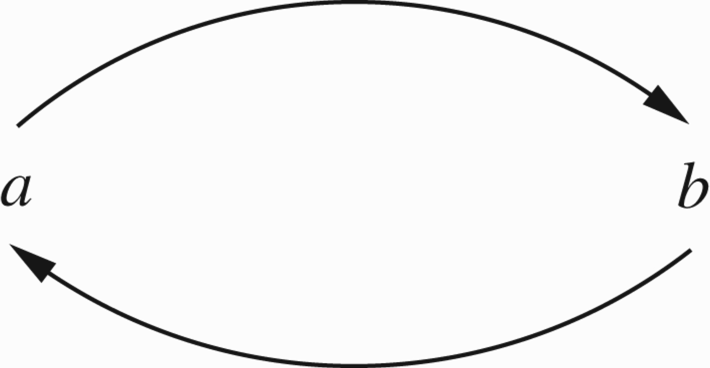
Suppose we have in the world w, the case that ◊ q attacks p (i.e.
On the other hand, we also expect that for some w′ such that wRw′ we have
We get an internal incompatibility in the system. Obviously we need an internal device to deal with this either an additional compatibility postulate or by something else. We solve this problem by introducing the concept of usability. We have a usability function hw and we have in this case
Of course, there is independent motivation to the concept of usability. Its introduction is not just technical.
In the above considerations, the dominant view was that of modal logic, and the argumentation network view was auxiliary; it provided a means of defining ⊨. Can we look at the entire possible world system as one big argumentation network? Put differently, can we view
This is possible to do using auxiliary arguments which eliminate R and W. We first explain this by example. Consider Figure 1. There are three worlds w, w1, w2. We have wRw1 and wRw2. We assume the grounded extension in each world. ◊ q is not attacked in w1. It says that it is possible to have an accessible world in which q holds. So, we must have either q in the grounded extension of world w1 or q in the grounded extension of world w2.
Figure 1.
Example for eliminating R and W.
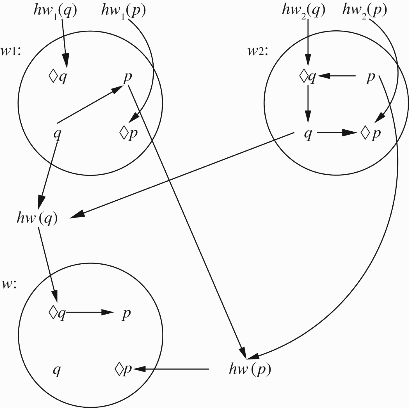
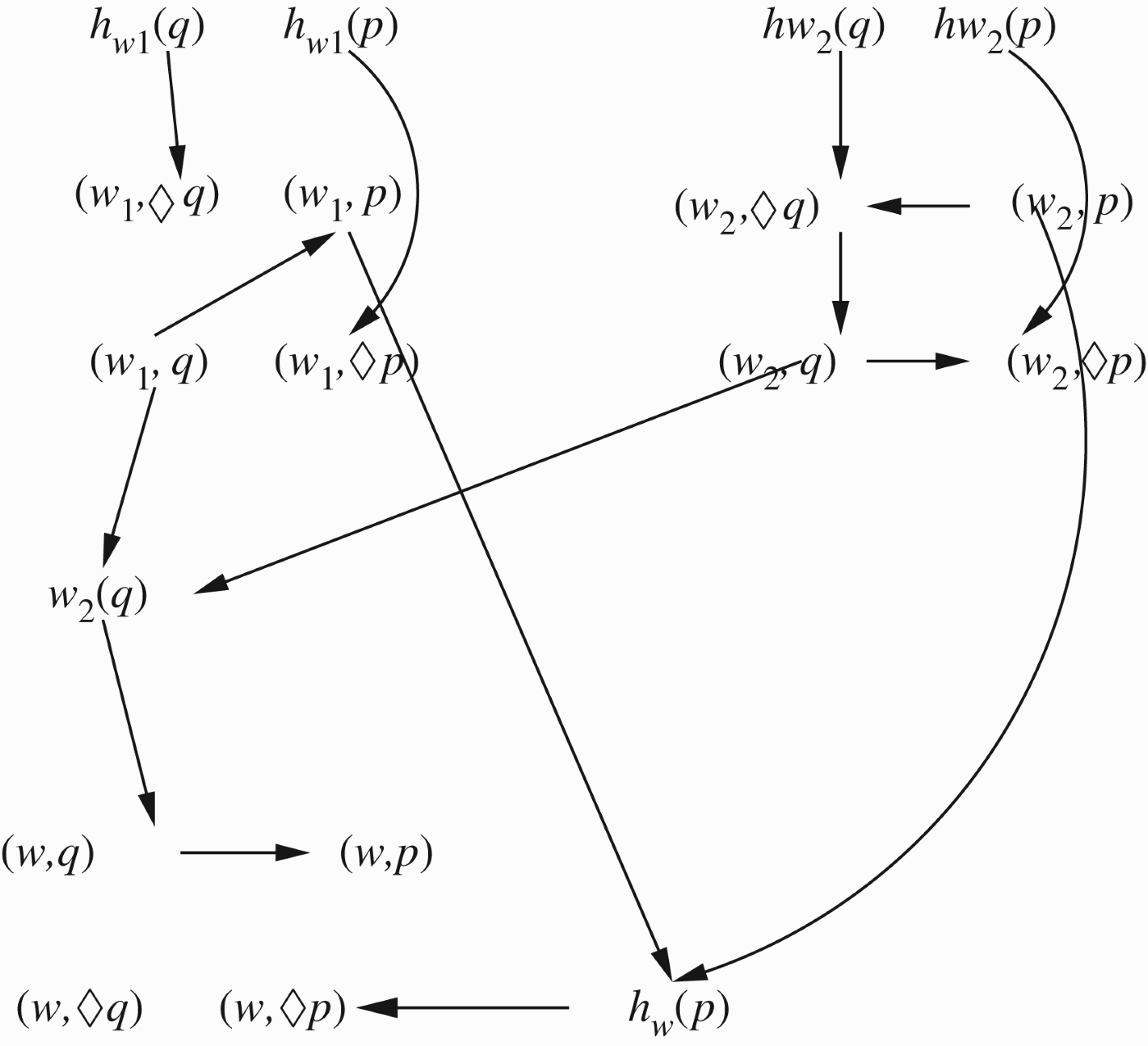
If this holds, we say ◊ q is usable in w, otherwise not. This usability is implemented in the object level by adding the point hw(q) as a meta-point outside the possible worlds, which point attacks ◊ q of the world w, and letting all the qs of the accessible worlds attack it. By the traditional rules of Dung argumentation, if at least one of the qs in w1 or in w2 is in, then hw(q) is out and so ◊ q is in. Otherwise, ◊ q is out (not usable) in w. We do the same trick for ◊ p. If we want to eliminate the big circles indicating the worlds, we have to annotate the atoms by the world name. If we do that we get Figure 2, which is one big uniform argumentation network where we seek the grounded extension.
The above discussion shows what options we have in principle in formulating modal and temporal argumentation networks.
(1) Let modal logic dominate by keeping the possible worlds separate and allow for an argumentation network to say what holds in each world.
(2) Incorporate the modal aspects inside one big argumentation network by using auxiliary meta-arguments. This way we are compiling modal logic into argumentation. This is technically possible to do, even possible to do nicely, in view of the results in Gabbay's (2011) paper, showing that argumentation is equivalent to classical logic in a nice way.
(3) In the temporal logic case, there is a simpler and more immediate way of defining a temporal logic network. We simply time stamp each argument with a moment of time or an interval of time, these being the times when this argument is considered usable. Thus, a network has the form
where τ(x)= moments of time, where x is usable.There is a very simple model, used in 2005 in Barringer, Gabbay, and Woods (2005), in connection with temporally varying numerical strength of arguments.
In itself, the model is too simple and does not offer much, but one can easily add natural structure to it to indicate evolution over time, as done in Barringer et al. (2005) and Abraham, Gabbay, and Schild ((2011a, b). In Barringer et al. (2005), the change in time was of strength of argument and this can influence the argument's attack capabilities and (Abraham et al. 2011a) the time stamping was used to resolve loops.
2.Introducing the global meta-level approach to temporal networks: concept of usability
There are several good reasons why we should consider modal and temporal argumentation networks
(1) Temporal facts as arguments. Past facts or future scheduled events can also be used as arguments for the present. An argument against the trustworthiness of a person may be the facts of past betrayals. An argument in favour of a higher mortgage loan may be a scheduled increment in salary next year. Unfortunately, this does not work with UK banks. An argument against a higher mortgage loan may be the possibility of redundancy in the future. Figure 3 is an example of how a scheduled redundancy exercise in the near future can be used as an argument against a high mortgage loan now, where d means the event of redundancy and m the general argument in favour of a mortgage.
We shall discuss later why it is not reasonable to encapsulate ‘Future d’ as a single argument c attacking m now. We lose structure this way (compare with how we lose structure in propositional logic in case
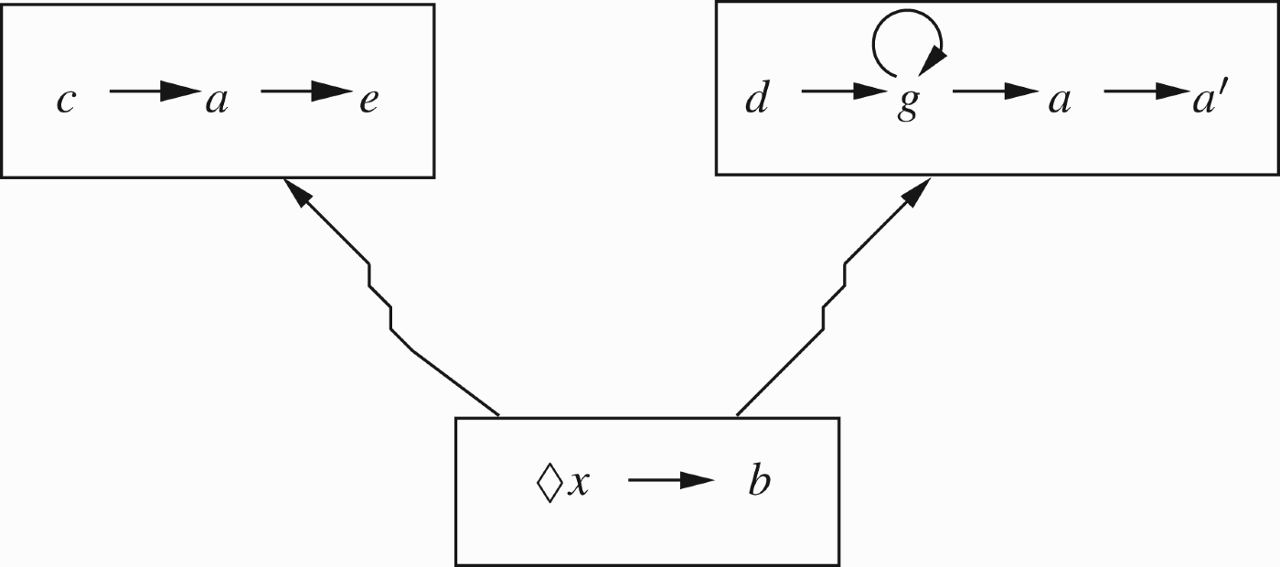
(2) Fibring arguments. Arguments from one domain may be brought into another domain. For example, expert medical arguments may be brought in as a package into a legal argument. This may be best treated in the context of modal logic (bringing information from the medical world into the legal world), where ◊x means bring in information x from another world, i.e. domain. See Figure 4. Let b be the legal argument to commit the accused to a 1-year prison sentence for tax evasion. Let c be the medical argument that the accused has cancer. This medical argument attacks b in the legal world. A hefty fine is more appropriate. c is part of a medical network of arguments and c emerges among the winning arguments of that network. Figure 4 illustrates the situation. Of course, in the legal world ◊c might be attacked as unacceptable evidence on the basis of some procedural errors in putting in forward (not shown in diagram).
(3) Future arguments. The possibility that an argument a may be able to defeat another argument b. We denote this by ◊ a. Such possibilities are central to threats and negotiations’ arguments where various future scenarios are discussed. For example, do not ask for more than a 10% salary settlement as it will never be approved by the executives – there may be strong fairness arguments for claiming 10% but pragmatically it will not be affordable and thus will not get approved.
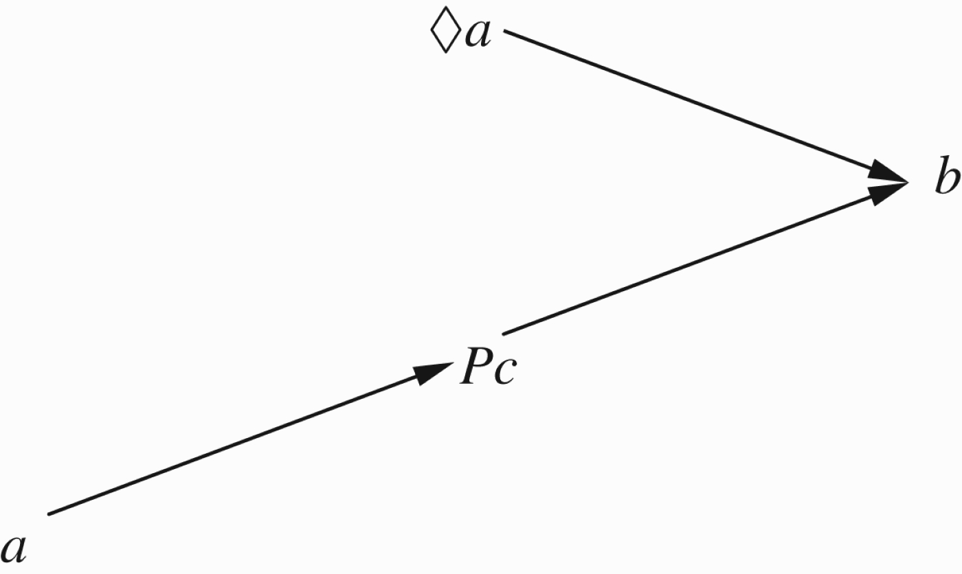
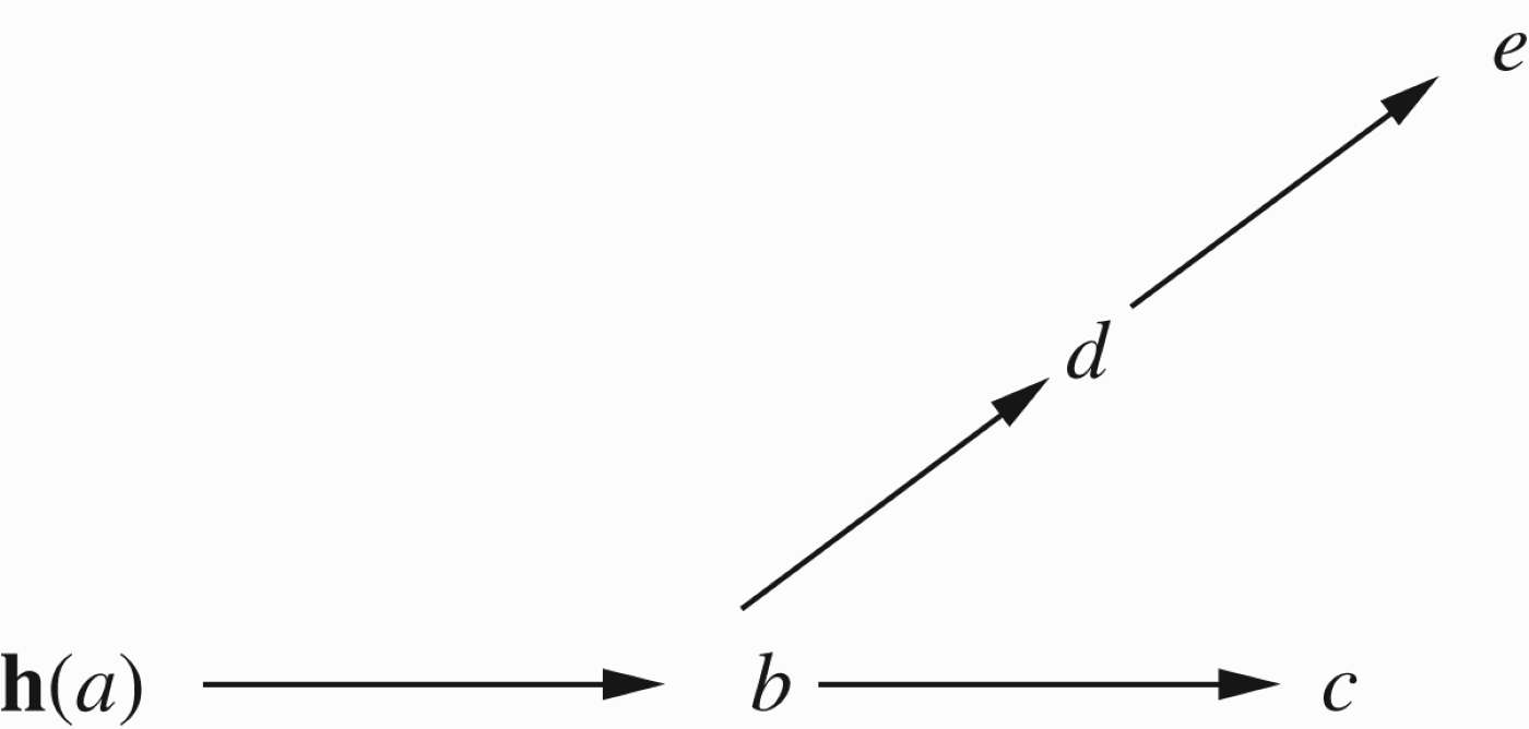
(4) Past arguments. We can use the fact that an argument c was potent in the past (denoted by Pc) to attack another current argument. Figure 5 is an example of such a configuration, where ◊ a indicates that argument a is possible and Pc indicates that argument c was considered in the past, but maybe is no longer taken seriously now, yet the fact that it was a serious argument in the past is sufficient to defeat b. For example, a mother might say ‘I have always cared for you, you cannot abandon me now’.
For example, a female employee may threaten with a possible argument claiming harassment. It may be that one cannot argue harassment now but it is not clear what the circumstances would look like when reviewed in the future. So, ◊harassment may have some force. We have had many such arguments when UK law was expected to be overruled by EU law. Many ◊(EUlaw) arguments were already defeating local UK arguments even before the EU law came into force in the UK.
Negotiations always involve evaluation of future scenarios of possible arguments and counter arguments and the possibilities of certain scenarios may be a strong argument at present.
Arguments from the point of view of tradition have always been successful in the past, e.g. we have always accepted the A'level standard as an appropriate university entrance qualification, so we continue to do so, even though many will argue that the level has dropped. We can have our doubts about the value of tradition now but yet an argument of the form ‘but it has always been the case that x’ may still win out.
Any use of precedent is also akin to this form.
Figure 3.
Future used as argument against present.
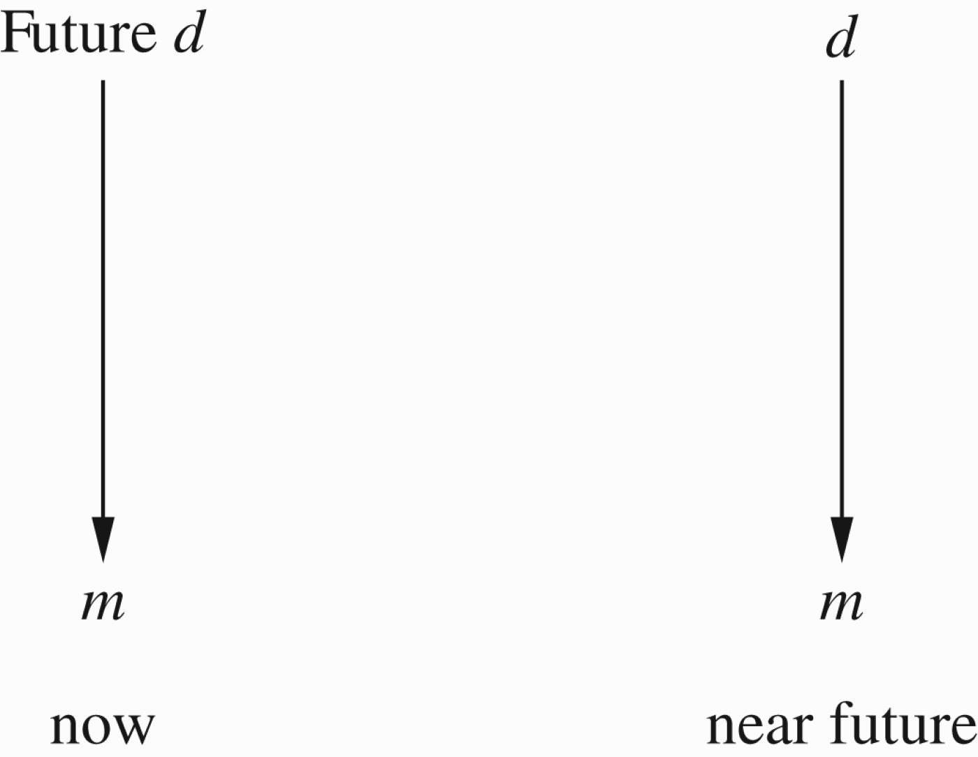
Figure 4.
Fibring arguments.
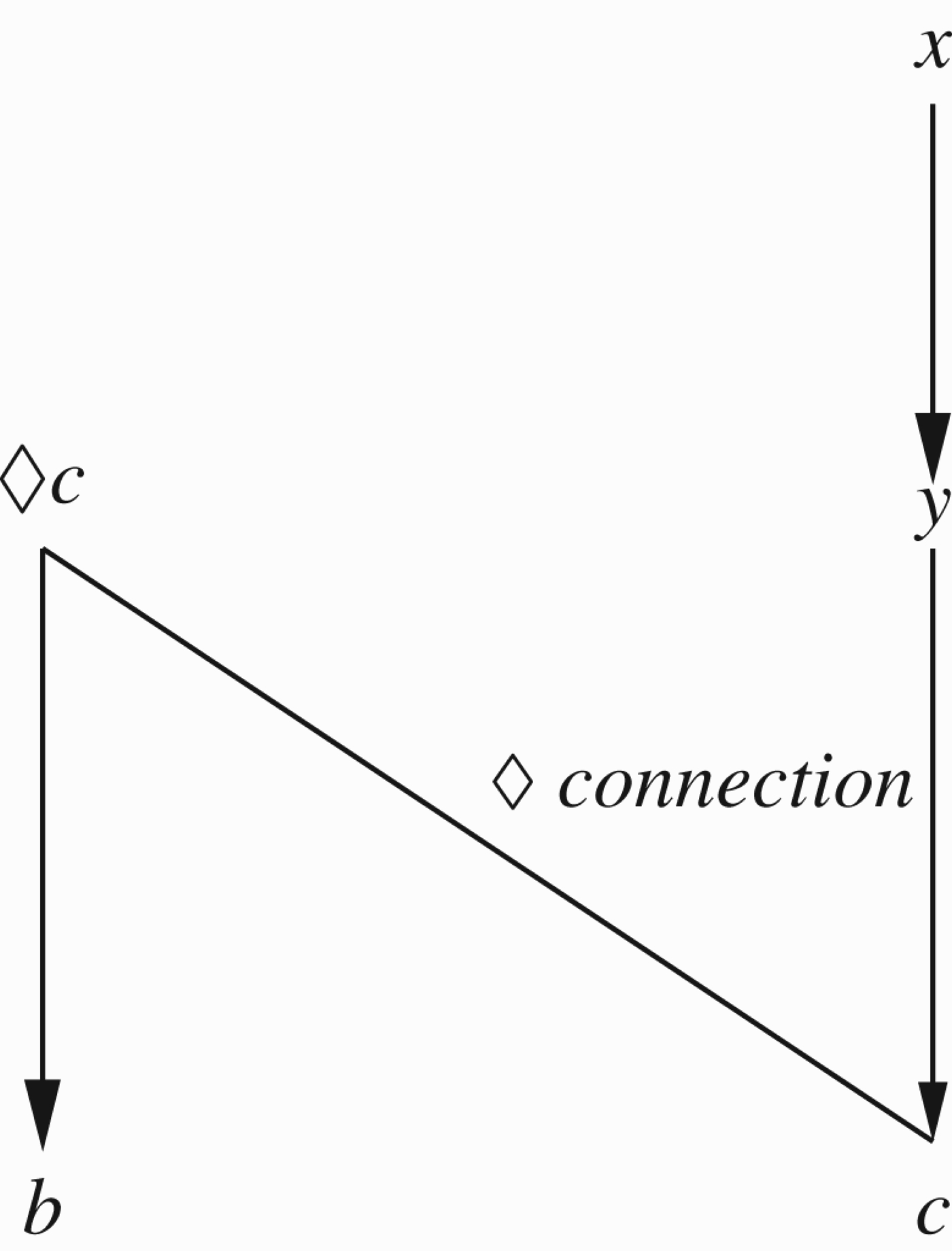
Figure 5.
Using a past argument to attack a present argument.
The basic notion is that of admissible extension. This is a subset E ⊆ S such that
(1) E is conflict free, i.e. for no x, y∈E can we have (x, y)∈R.
(2) E is self-defending, i.e. for all x, y∈S, if x∈E and (y, x)∈R, then there exists a z∈S such that (z, y)∈R.
The above discussion suggests that we introduce the concept of usability of arguments. We may have at a certain time or at a certain context some arguments that are talked about and are available in some real sense, but these arguments cannot be used for a variety of reasons. The formal presentation of such arguments can be to introduce them into the network but label them as unusable through a usability function h. If x is an argument, then h(x)=1 means it is usable and h(x)=0 means it is not. The reader may ask why do we want to introduce them at all if they are not usable? Well, in the context of modal and temporal logics, it makes sense to talk about them. Maybe they were usable, maybe they will be usable or are possibly but not necessarily usable, or should have been usable, etc. We give several examples.
Example 2.1
Example 2.1The catholic super administrator
A UK university, operating an equal opportunities policy, advertises for a faculty administrator. There is a shortlist of three candidates and, because of a special request from one candidate, the interview date is moved.11
The top two candidates are: a woman aged 42, who knows 15 languages and 10 computer languages and has a PhD in economics and business administration from Harvard. She has lots of experience working for government administration; the other candidate is a man of similar age, but not with as strong a background as the lady.
There is an argument for hiring the lady candidate: she is the best!
There is an argument against hiring the lady candidate: she is Catholic, aged 42, recently married, and will probably waste no time in starting a family.
This latter argument is a strong subjective argument, which, following the proper procedures, cannot be used. Indeed, one cannot mention it, let alone even think it! h (this argument) =0.22
Example 2.2
Example 2.2The rape
A girl complained she was raped by a man late at night in the street. The man claimed that she gave him reason to take the view that she was willing and available. The entire incident was filmed, video and audio, by a CCTV camera.
However, this camera was installed without a licence and hence, because of a legal technicality, any evidence from the CCTV is not admissible. The evidence from the CCTV clearly and unambiguously defeated the claim of the man, but because of its inadmissibility, the jury was instructed to accept the man's claim.
In both cases, we present the network in the traditional form (S, R), where S is the set of arguments and R is the attack relation, but with both usable and unusable arguments included, where those that are usable are marked via a function h. h(a)=0 means we cannot use argument a. h(a)=1 means we can use the argument.
It is important to note that unusability is temporary and can change. Circumstances can change, the law can change, new arguments can be brought forward and what was unusable can become usable.
(1) Unusability due to defeat. Figure 4 can be an example of unusable argument. The notation ◊ c, wants to bring the cancer argument from another network, the medical network into the present network, the legal one. In the figure, c is a winning argument in the medical network and it is attacked by y in the figure but is defended by x. However, it is quite possible in a complex cross-network situation, that we have a ◊ z such that in the appropriate network for z, z is defeated. In this case, we can view ◊ z as unusable. Again, this is not permanent and may change.
(2) Unusability due to secrecy. It is quite possible that an argument a is defeated by an argument a* which cannot be recorded explicitly in the system. In this case, it may be convenient not to mention a* and to simply mark a as unsuable.
3.Temporal networks: formal considerations
We need to define the formal machinery and distinctions allowing us to put in context our approach to modal and temporal argumentation networks. So, we define some basic notions in this section and move on to the Kripke models in the next section.
Definition 3.1
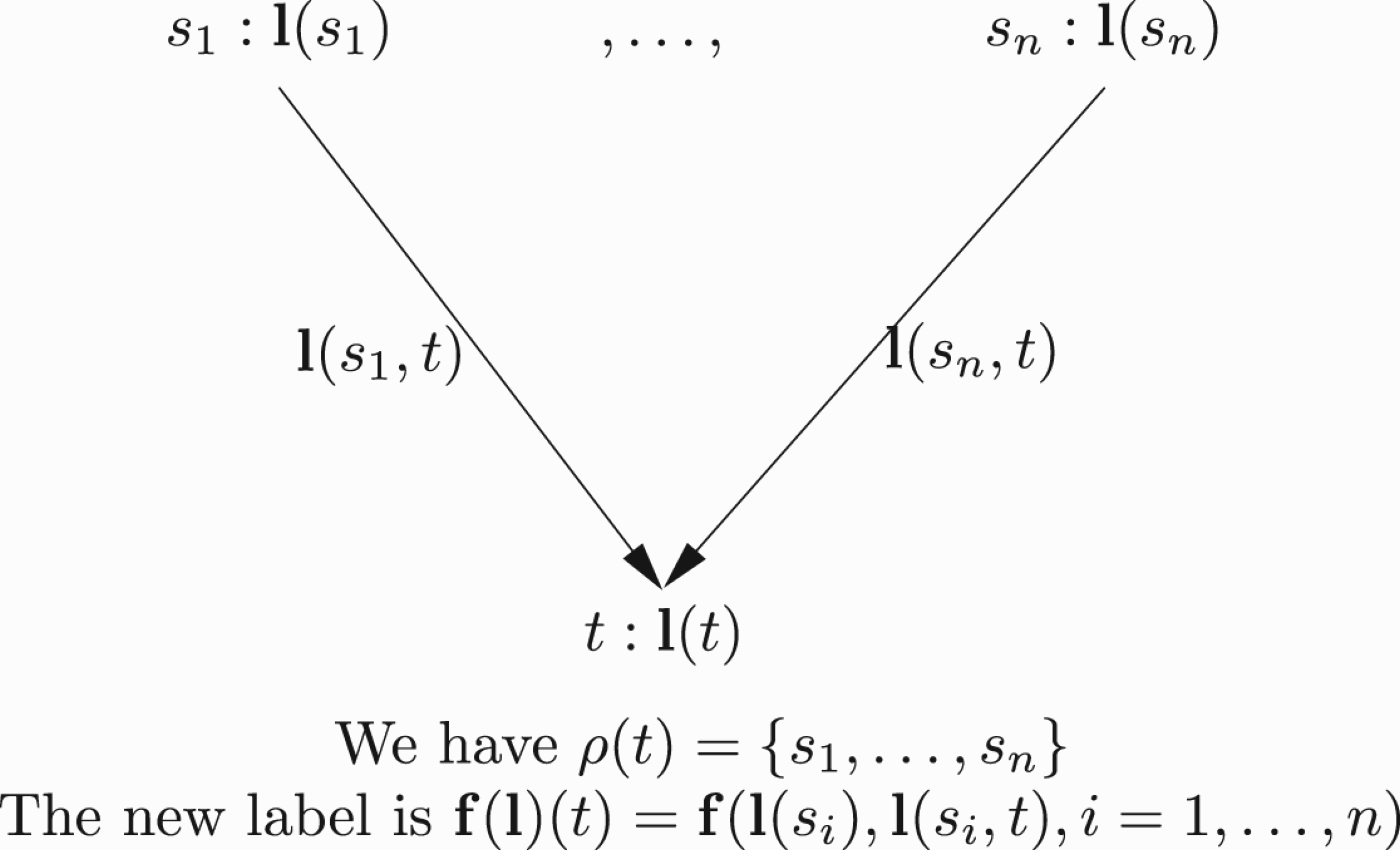
Definition 3.1General labelled networks
(1) A general labelled network has the form
where T is a set of nodes andThe functional f is an update functional, it updates the labelling function l to a new one
be new labels at t, and at(s, t) given by the functional f. f depends on ρ andThe way f is calculated is not described here. The reader can compare later in the section below, where we give some examples of algorithms for f in terms of ρ and l .
(2) f can be used for successive updating of the labelling of our network.
We define
Step
Step
Let ? be a fixed label in 𝕃. We can define
We now have the machinery to look at argumentation networks and we use the Caminada labelling for them (Caminada and Gabbay 2009; Caminada 2011).
Figure 6.
A general labelled network.
Definition 3.2
Definition 3.2Argumentation model
(1) Let ℂ be the language of the classical propositional calculus with atoms Q and connectives
(2) An argumentation model has the form
(3) Given h, we can assign usability values to the formulas of 𝔽 using the traditional truth table. We write h(A) as the value of a wff A under h. h can now be regarded as a subset of 𝔽.
(4) A network is atomic iff
(5) Note that h gives initial usability values which are not necessarily permanent and may change in the course of the recursive evaluation, see Definition 3.3.
Definition 3.3
Let
Level 0
h0(A)=h(A).
Level m+1
Let
(1) hm(B)=0 for all B∈ρ (A). In this case, let hm+1(A)=1.
(2) For some
(3)
Level ∞
Let
Let
h∞is called the BG labelling of 𝔽.
Definition 3.4
Definition 3.4Caminada labelling
Let
(1) if
(2) If for some
(3) If for all
(4) If for some
Lemma 3.5
Let
Proof
Let h+(x)=1 if
Let h+(x)=0 if
Let h−(x)=1 if
Let h−(x)=0 if
Let h0=h+.
We now prove
(1) If hm=h+, then hm+1=h−.
(2) If hm=h−, then hm+1=h+.
If
If
If
Clearly if hm=h±, then
If hm=h+ then hm(x)=1 and
This shows that hm+1=h−, since x was arbitrary.
If hm=h− then hm(x)=0 and
Again since x was arbitrary, we get hm+1=h+.
So, if we start with h0=h+, we get h2m=h+, h2m+1=h− and so
Lemma 3.6
The converse of the previous lemma does not hold. Not every h∞is a Caminada labelling.
Proof
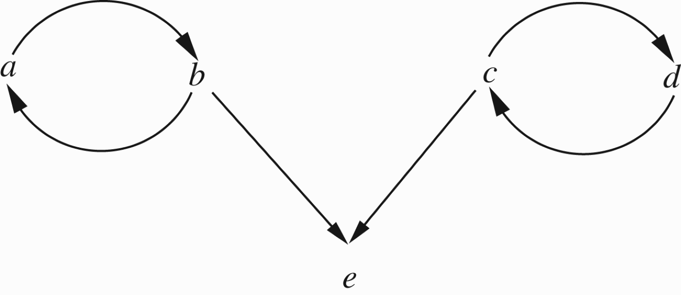
Consider the network in Figure 7
Figure 7.
Oscillation and attack.
Start with
We also have
The Caminada labelling rules do not allow for
Remark 3.7
(1) The reason we could provide the example in Figure 7 is that h gave value 1 to the loop (a, b) and value 0 to the loop (c, d). So, as the values in the loop oscillated, there was always one loop which attacked e. If all loops were to oscillate synchronously, h(e) would have oscillated as well.
How can we overcome this? We can use ultrafilters to get an exact value out of the oscillation. We need some concepts
Let ℕ be the set of natural numbers. A family of subsets 𝕌 of numbers is called an ultrafilter if the following holds
𝕌 says which sets are ‘big’.(a)
(b) If
(c) either X or ℕ−X is in 𝕌.
We also note that there exists an ultrafilter 𝕌 such that all co-finite sets are in 𝕌.
We now give an alternative definition of h∞. Call it hω.
Let us see what happens with the example of Figure 7 if we use hω instead of h∞. We haveUa=Ub=all even numbers.
Uc=Ud=all odd numbers.
One of two sets {odd numbers, even numbers} is in 𝕌. From symmetry, we can assume without loss of generality that it is the even numbers. We get
So hω is the same as h0 and we have nothing.Let us try another angle.
(2) The discrepancy with the Caminada labelling and hence with the Dung network rules seem to arise in the case where a winning argument x according to Dung gets a value h(x)=0.
Figure 8 gives two typical examples.
Figure 8.
Example showing the discrepancy with the Caminada labelling.
According to the Dung rules a, d, c are winning arguments. If h is such h(a)=0, then b and e will be the winning arguments.
The question we ask is can we use a device which makes the two approaches compatible?
Suppose we say a is not usable (i.e. h(a)=0) because there is an attack on a. Say
The above trick works for this network. Does it work in general?
Given an atomic network
Do we have a general theorem that we can pair the winning subsets? I.e. can we have:
We can hope for such results only if whenever h says an argument x is out then it is out permanently, because when we insert(a) For any winning set
(b) For any winning set
Our algorithm in Definition 3.3 and later on in the section dealing with modal and temporal logics, does not keep unusable arguments out permanently, it does bring them in depending on the attack cycles.
Remark 3.8
Remark 3.8Discussion of the Dung network rules
(1) The discrepancy with the Caminada labelling is a serious one. The Caminada labelling is faithful to the Dung argumentation network rules, namely (Definition 3.3)
In the Dung framework, these rules are not defeasible rules, they are absolute.(a) If all attacks on a node x are defeated (are out), then x is in.
(b) If some attacks on a node x are in, then x is out.
(c) If there are no nodes attacking x, then x is in.
So consider, for example, an argumentation network with one node and one argument x. Since nothing attacks x, x is a winning argument. If we look at a classical model for x with x=0, namely x is unusable for whatever reason, then the Dung rule overrides the unusability of x and x is still a winning argument.
Compare this with default logic. The default rule x/x says that if x is consistent to add then add it by default. This will not override any given data about x.
So, rules (a)–(c) are too strong when we give a model interpretation to the arguments. An argument can win even though it is unusable, simply because it is not attacked.
(2) We call for a new critical evaluation of rules (a)–(c). We would abandon rule (c) and modify rule (a).
The proposed BG rules for a Dung network relative to an assignment or other evidence are (a*)–(c*) below. We call the associated update functional π* (compare with π of Definition 3.3).
Jakobovits and Vermeir (1999) have already proposed that an argument which has all of its defeaters out need not necessarily be in. This view is criticised in Caminada (2006). Our (a*) and (c*) are in line with Jakobovits and Vermeir (1999).(a*) If all attacks on x are defeated and there is no evidence that x is unusable, then x is in
(b*) If some attacks on x are in, then x is out.
(c*) If there are no nodes attacking x, then x is in only if there is no evidence that it is unusable.
(3) Let us call an assignment h a Caminada assignment to the atoms of Q if for some Caminada labelling λ we have
From Lemma 3.5, we know that• h(x)=1 if
• h(x)=0 if
•
Remark 3.9
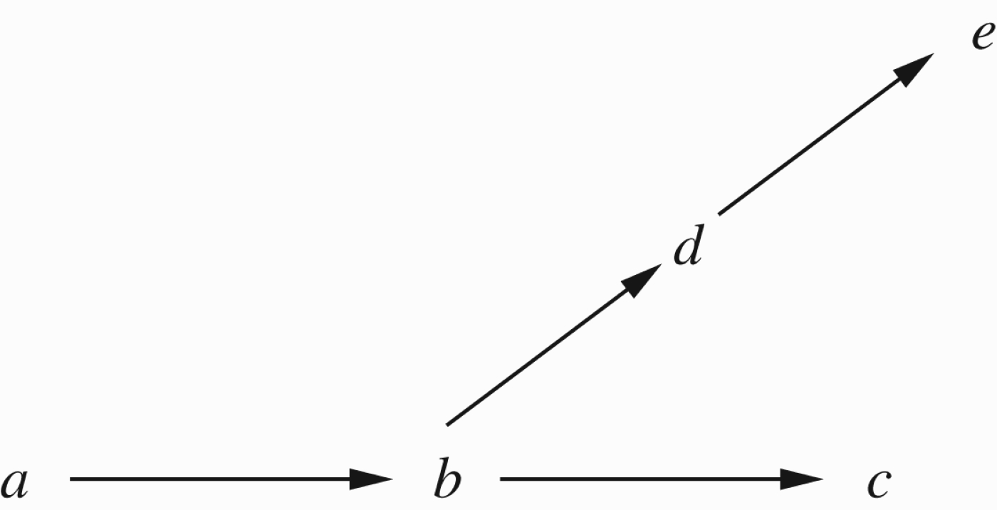
The difference between BG and Caminada labelling can be appreciated by looking at the logic programming translation of a Dung network. Consider the network
(1) b if ¬ a.
(2) a.
(1*) b if
(2*) a if
(3*)
(4*) zero(x), for all x such that x= usable, under the assignment h.
Note that we use
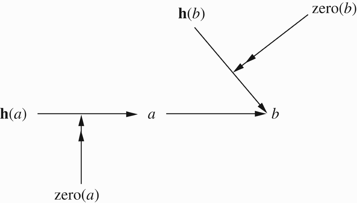
The corresponding Dung network for the above network is Figure 10 (Footnote 1):
Figure 10.
The network of Remark 3.9.
So, the BG programme is defined to contain the following clauses
4.Kripke models for argumentation networks 1
We begin this section with some methodological remarks and general examples which will bring us to a point of view best suited for the presentation of modal and temporal argumentation networks.
We begin with a simple example. Consider the sentence
• John read le livre with interest.
Now consider
• John is dishonest because he did not pay yesterday.
Let t label the location of the main sentence and let s label the location of where we need to go. In each case, we have the following situation.
In the process of evaluating the algorithm 𝒜t at t, we hit upon a unit of the form
Take x to location s, find a value
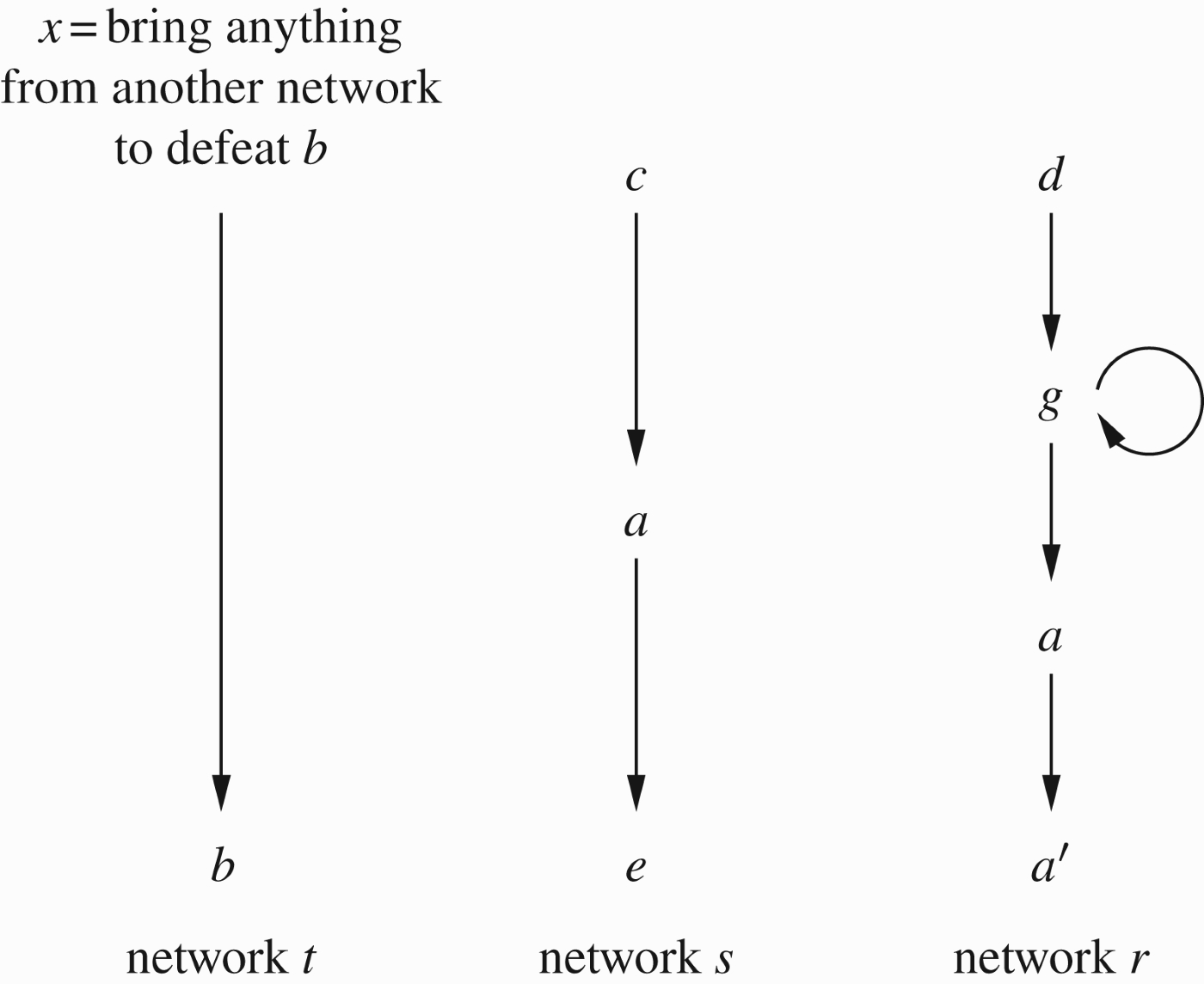
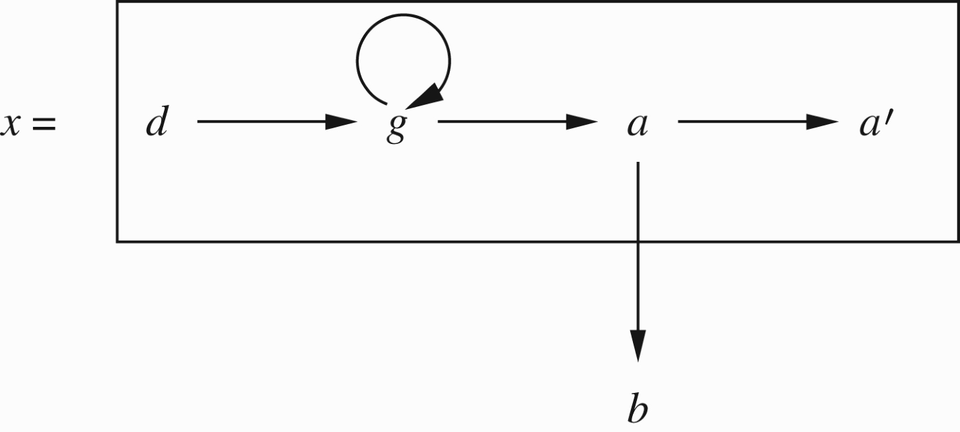
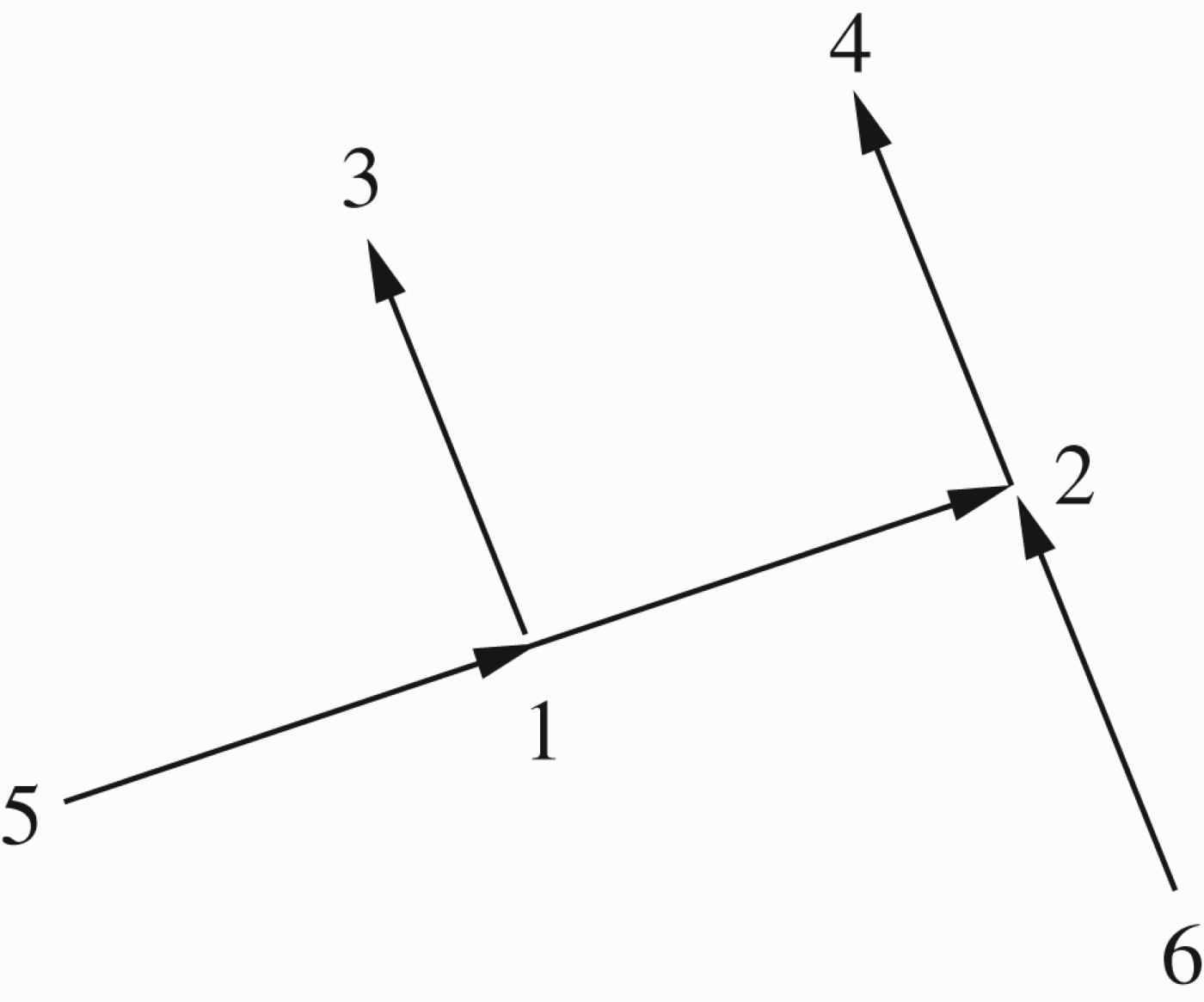
Let us now take another example. Consider the three argumentation networks in Figure 11. In network t, the node x is not an argument but an instruction to look for an accessible network in which there is a winning argument which can defeat b. The two accessible networks are s and r. In s, a is not a winning argument, but it is in r. Suppose a is capable of defeating b; this knowledge is not recorded in the network t but is known to us either extra-logically or intrinsically (for example, b is logically inconsistent with a). Then, x will be instantiated as the argument a coming from network s. x, being an instruction or a recipe for finding arguments, can be as specific as needed for a successful search. Note that we could have written Figure 12 instead of Figure 11. This is a fibring of network r at position x at network t. The attack on b comes from inside the network r from node a onto node b (in network t).
Figure 11.
Networks related by instructions.
We can turn the situation into modal logic by using ◊ x (or even ◊ a if we know that x=a will do the job) and we get a kind of Kripke model, see, for example, Figure 13. The zigzag arrow ↭ is accessibility and the ordinary arrow → is attack. ◊ x (or ◊ a) means find a winning argument a which can attack b. Here, the meaning of ◊ a is administrative. ◊ is a meta-level administrative connective. ◊ a does not mean that a is a possible argument; and ◊ is not in the argument language.
Consider now the following network
◊ storm→b
Technically, the mathematics of both cases, the administrative meta-level ◊ and the temporal event object level ◊, is very similar. In both cases, we can put ◊ x in the nodes of an argumentation network and seek winning arguments in accessible networks.
In either case of ◊ x, we need to search other networks for an appropriate winning value. So, it is not clear until after the calculation and search, whether we have a usable argument here or not, especially if the family of networks is complex. Hence, the need and the technical usefulness and value of a usability assignment. It simplifies matters during the calculations.
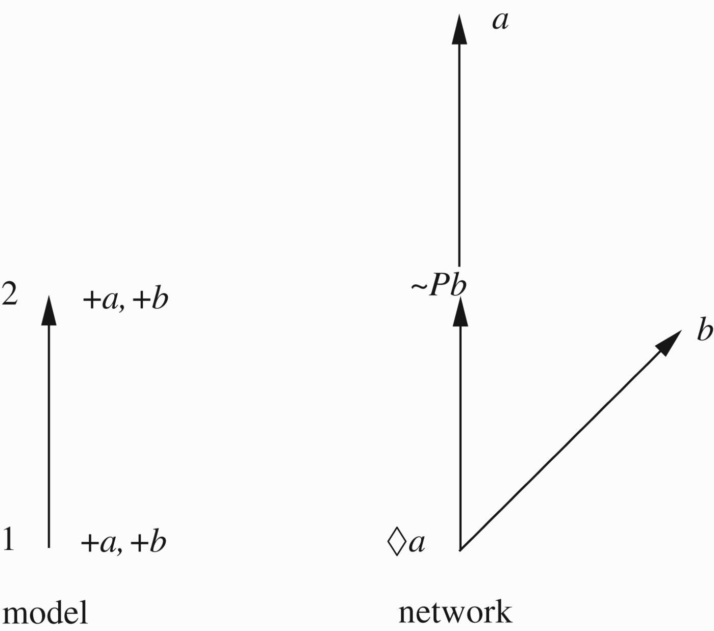
We now explore our options for Kripke models for argumentation networks. We begin with a simple first attempt which will turn out to need improvement. However, it is helpful to go through this first attempt for us to appreciate what is to be added. Consider the network of Figure 5 and let Figure 14 describe a Kripke model. The reader should bear this in mind when reading the next formal definition.
Definition 4.1
Definition 4.1Languages
We recall here the languages of modal and temporal logics.
(1) The classical connectives we use are ∼ (negation),
(2) In temporal logic, we use the connective PA which for A was true in the past and FA for A will be true in the future. A temporal model is usually presented through a nonempty set T of moments of time and an earlier-later relation < on T. < is usually taken as irreflexive and transitive. The classical truth conditions for P and F are
• t⊨ PA iff for some s such that s<t, we have s⊨ A.
• t⊨ FA iff for some s such that t<s, we have s ⊨ A.
Temporal logic defines
(3) Modal logic uses ◊ A reading, A holds in another accessible world. The set of worlds is denoted by S and has an accessibility relation
•
□A usually means
(4) The usual temporal or modal logics have formulas evaluated at worlds. If we want to define the notion of modal and temporal networks, we will need to deal with networks of formulas evaluated at worlds.
(5) We can have in the language both the temporal connectives P, F and the modal connective ◊. In which case, the semantics will need to have both R and <. We may allow for the future to be also a possibility for ◊, in which case we have:
Sometimes only P and ◊ are used in which case we can use only R and go backwards in it for evaluating P.(6) The examples below use ‘usability’ instead of truth. So, we have for an example that ‘a is usable at world t rsquo; is treated mathematically the same way as we treat ‘ a is true (holds) at t’.
Let us start with some examples in the simple language which contain arguments of the form x, (atomic), ◊ x, possibility of an argument, and Px, past arguments. Think of ◊ x as future possibility. So, in the Kripke model, ◊ goes up in the arrow direction and P goes down in the arrow direction.
In the usual Kripke evaluation procedures for classical logic, with a set Q of atomic arguments, we have an assignment h giving a truth value at each world t for each atomic proposition q. We write
So, we give the following definition. For each node n in the Kripke model, we assign a set
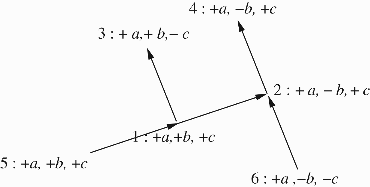
Figure 15 is an example of such an assignment, where we write ±q to indicate the value of q.
Figure 15.
An example of an assignment.
Suppose we want to know the value of the network of Figure 5 at the model at node 1. How do we evaluate Pc? We follow the traditional steps of evaluation in a Kripke model; we go down the accessibility relation and look for a world where c is usable.
At node 5, we have +c, so maybe we say +Pc at node 1, but we notice that a attacks Pc in the network (Figure 5). So, does 1⊨ Pc or not? Furthermore, Pc attacks b and so at node 2 does Pb hold or not?
We have +b at node 1, so we would like to say 2⊨ Pb, however b may be successfully attacked at node 1. So, we may not have Pb after all, so what do we have?
We need an agreed recursive definition.
Let us see some examples where we might have a loop, and try and get a clue by working the example out.
Example 4.2
Consider the network and Kripke model as described in Figure 16
Figure 16.
A model for Example 4.2.
To evaluate the network at 1, we know that
So, we need to know the value of b at 1. We do have +b at 1 but this is attacked by ◊ a so we need to know the value of a at 2 and we have a loop.
We need some process of evaluation which will give us a better chance to resolve the loops.
We do this by levels of recursive evaluation. We use two bits of notation.
(1) hm (t, A) is the assignment of value at level m to the argument A. A may be atomic or a formula.
(2) t⊨mA is the network value of A at world t at level m. We use the BG algorithm for the functional π* namely clauses (1*)–(3*) of Remark 3.8.
So to make the meaning of hm and ⊨m crystal clear: hm says which arguments in the network are usable at level m, while ⊨m says which arguments are winning (not defeated) at level m. An argument defeated at ⊨m is considered unusable by hm+1.
Let us now apply this to Figure 16’s example.
Level 0
h0 is the assignment h to the atoms as indicated in the Figure, i.e.
For
It is convenient to use the notation
Level 1
Level 2
The assignment we use to calculate h2 is the atomic part of ⊨1, namely 1 ⊨1a and
Level 3
⊨2 gives us a new assignment to the atoms, namely 1⊨2a and 2⊨2b.
Level 4
We now get the assignment from ⊨3 for atoms as
Remark 4.3
The reader may wonder what has happened to the loop we observed before and what kind of interpretation (loop resolution) we are getting. To explain that let us look at the traditional loop in the network of Figure 17, in which a and b attack each other. We have three complete extensions
Figure 17.
A traditional loop for Remark 4.3.
Let us do the level calculation intuitively.
Level 0
Start with +a,+b.
Level 1
Attack as suggested by level 0. We get −a,−b.
Level 2
Attack as suggested by level 2. We get +a,+b.
So, we are infinitely looping and we can put a question mark on a and b, leading to ∅.
Of course, everything depends on the assignment at level 0. Other possible assignments are
Example 4.4
We try and evaluate the network of Figure 5 at the model of Figure 16. We use the BG π* evaluation algorithm.
We do this by levels. Let h0 be the assignment to the atoms as indicated in Figure 15. Thus, h0 satisfies
Level 0
We evaluate h2 using the assignment to the atoms suggested by ⊨1.
Definition 4.5
Definition 4.5Temporal languages
Let Q be a set of atoms. The basic temporal language based on Q uses the unary connectives
The language is said to be very basic if we allow ◊ x and Px and x only.
The full temporal language also allows the use of the classical connectives
Definition 4.6
Definition 4.6Temporal Kripke models
Let (S, R, a) be a Kripke model and let
We define by induction a sequence of new assignments h1, h2, … and semantic consequences
(1) Let h1 be defined as follows
h1(t, PA)=1 iff for some s, such that sRt we have h1(s, A)=1.
The definition for the classical connectives is the usual one.
(2) Let ⊨1be defined as follows:
First consider h1(t) as an assignment on
We define ⊨1by
The reader can compare with the construction in Example 4.2.
We now define
hm+1 is obtained from ⊨m in the same way that h1 was obtained from h, by regarding
⊨m+1 is obtained from hm+1 in the same way that h2 was obtained from h1, i.e. for each t, we have
This defines hm⊨m for all n≥1.
We now define
Otherwise if t⊨mA oscillates, we say that
5.Kripke models for argumentation networks 2
Let us assess the situation we are in. In the previous section, we offered a simple model. This model can be improved. The problem is not so much the discrepancy with the Dung approach (Remark 3.9) as this is not a unique possible world problem, but the difficulty is that we need to sharpen the intuitive meaning to Definition 4.6. It is mainly technically motivated by a natural formal analogue of the semantical movements in a traditional modal and temporal Kripke model. We need to clarify more sharply the meaning of usability of arguments and its connection to truth and falsity and possibility of argument and facts.
There seems to be a fundamental difference between the modal operator ◊ and the temporal operator P. P goes into the past, while ◊ goes to an alternative world of different reasoning/argumentation framework. In an ordinary Kripke semantics for traditional modal and temporal logics, there is no technical distinction between the two. In an argumentation context, we need to give different technical treatment to these two connectives. The ◊ we treat as a fibring operator (go to another context, do something there, and come back with the result, see Gabbay (1996)), while the operator P is still treated as purely temporal.
We illustrate with an example.
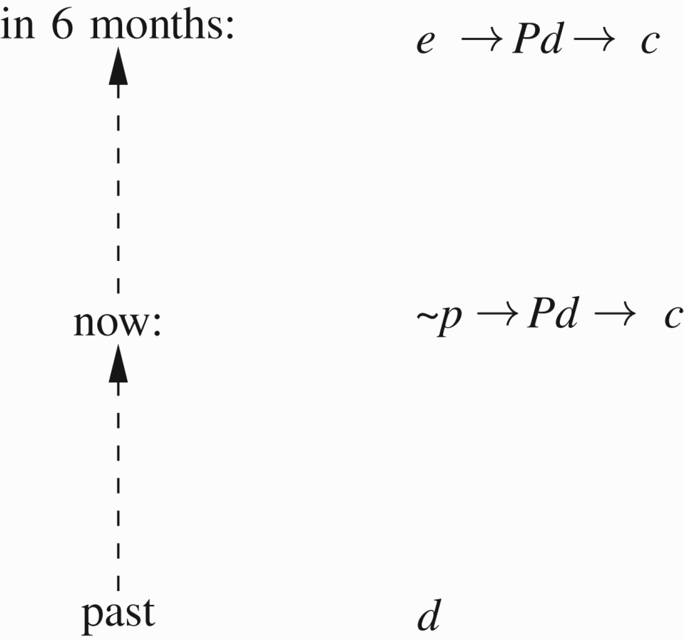
We want to argue against a political candidate c. We want to bring in the past facts that he double-crossed his partners, showing lack of loyalty and trustworthiness (call this Pd, d for ‘dirt’). However, the situation today is such that digging up the past on a candidate is counterproductive (call this ∼ p). It is suggested therefore to wait 6 months for the facts to emerge naturally (i.e. ◊ d, where ◊ here reads future possibility).
A counterargument against waiting is that by that time criteria for judging candidates will change and the argument will be defeated, say d will be attacked by e (e can mean who cares?; it was a long time ago!).
Figure 18 shows the situation:
Figure 18.
A network with a temporal argument.
We notice the following discrepancies between the formal situation of Figure 18 and the formal definition we gave to modal and temporal argumentation networks in Definition 4.6.
(1) We have different networks at different possible worlds.
(2) ◊ behaves like a fibring operator
(3) P is purely temporal for facts.
(4) With P the assignment, h indicates ± usability by virtue of truth or falsity, while with ◊, the assignment h might indicate ± usability for other reasons.
(5) We cannot have a proper temporal and modal treatment of arguments without looking into the details of what is the internal structure of arguments and how exactly do they attack one another in terms of such structure.
Suppose we adopt the view that arguments are proofs and attacks disrupt such proofs. Let us examine how time T gets into the picture. Consider the following example:
I park my car near Russell Square at 11am in the morning, do my business of the day and come back to it at 5 pm. I expect to find it there. If I don't find the car then nonmonotonic deduction allows me to conclude that the car was stolen. We can have a little logical system (nonmonotonic or Bayesian net) which compares the conclusions of ‘car stolen’ against ‘car towed away by local council parking department’. We can assume the latter conclusion can be defeated. We can also ignore some well-known difficulties of persistence of arguments where one gets paradoxically that the car was stolen only a few seconds before my return (the stolen car paradox).
There is one sure way to attack this argument and its conclusion. This is to prove the simple fact that I do not have a car.
Figure 19 illustrates the situation
Figure 19.
Facts attacking an argument.
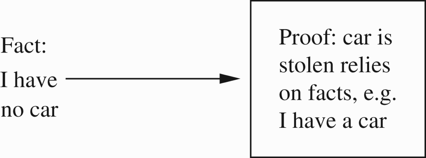
Facts can attack arguments most effectively. Also, if the facts are undecided or are not available, then we claim the argument is not usable. See Section 6 for further discussion.
So when designing a new modal and temporal logic for argumentation, we need a pure
(6) Our next question is whether an argument itself can be time dependent. This is a bit tricky. In monotonic logic, the answer is no. Euclid geometric proofs are as valid and good today as they were in ancient times. But in the nonmonotonic case, the answer is yes. Nonmonotonic reasoning depends on context. Today, a girl in a mini-skirt will not be considered immodest but go back 200 years and everyone at that time will nonmonotonically deduce she is ‘fast’. So as we can see from this example, the deduction mechanism itself can change in time. Thus, we may argue for example along the lines ‘you had better get yourself a decent long dress now because soon people's perception will change and you will no longer be respectable wearing a mini-skirt’.
Definition 5.1
Definition 5.1Temporal Kripke models – udpated
(1) Consider a language with the classical connectives
(2) A Kripke model for the above language has the form
(3) For each t, let
(4) We define by induction a sequence of new assignments h1, h2, … and semantic consequences
(a) Let h1 be defined as follows
h1(t, PA)=1 iff for some s, such that s<t we have h1(s, A)=1.
h1(t, FA) iff for some s such that t<s we have h1(s, A)=1.
The definition for the classical connectives is the usual one.
(b) Let ⊨1be defined as follows:
First consider h1(t) as an assignment on
We define ⊨1by
We now define
hm+1is obtained from ⊨min the same way that h1was obtained from h, by regarding
⊨m+1is obtained from hm+1in the same way that h2was obtained from h1, i.e. for each t, we have
This defines hm⊨mfor all n≥1.
We now define
Otherwise if t⊨mA oscillates, we say that
6.Conclusion and discussion
Modal logic deals with sets W of possible worlds w∈W. The possible worlds in propositional modal logics are usually atomic and have no internal structure. In this paper, we associate with possible worlds w argumentation networks of the form Nw. The argumentation networks Nw contain as arguments (i.e. the arguments appearing in the argumentation network Nw) modal and temporal formulas. Thus, to define extension in Nw, we need to look at extensions in other accessible worlds Nw′. This greatly enriched the language of argumentation but required a tricky inductive definition of how to calculate extensions and required the concept of usability of arguments. We also gave examples to motivate the need for such definitions, but we also discussed simpler definitions of temporal argumentation networks.
We continue with a comparison with some key papers. I am grateful to the referees for compiling this list.
(1) M.L. Cobo, D.C. Martines, and G. Simari, a 2010 paper on admissibility in timed abstract argumentation networks (Cobo, Martinez, and Simari 2010).
This paper offers a time stamping model, where each argument is time stamped when it is available. The model is similar but not the same as the ones used in Abraham et al. (2011a) and Barringer et al. (2005). In all cases, the change is in the meta-level. There are no temporal connectives involved.
(2) N.D. Rotstein, M.O. Moguillansky, A.J. Garcia, and G.R. Simari, a 2010 paper on dynamic argumentation framework (Rotstein, Moguillansky, Garcia, and Ricardo 2010).
The paper offers a model where arguments are based on evidence structures. Thus, the dynamics of change come from updates and changes in the evidence structure. There are no modal connectives in the object level to connect between different evidence structures.
(3) G. Boella, S. Kaci, and L. van der Torre, a 2009 paper on dynamics in argumentation with single extensions (Boella, Kaci, van der Torre 2009).
This paper does not offer dynamics of argumentation networks but rather principles in the meta-level which can govern change in networks. In particular, they offer properties for refinement of the attack relation. Thus, if, for example, we have an interrelated family of argumentation networks (different worlds or different times), we can check whether this family satisfies the meta-level principles offered in this paper.
Let us conclude with our plans for future research. What is interesting is to look at an argumentation network and partition the arguments into different subsets and regard them as subnetworks (i.e. different modal worlds) and put requirements on extensions as seen from the point of view of the different subnetworks. This presents a very neat way of introducing modality into argumentation.
Notes
1 As an argument for wishing a new interview date, the candidate has declared that she is getting married in the local catholic church, and these dates coincide. As a result of this correspondence, the interviewers know she is Catholic and a new bride.
2 There is a known case where a preferred candidate did not score as well as another candidate in an interview for a position in local government. In exceptional circumstances, the interview panel was reconvened and the outcome was that the preferred candidate's score actually fell!
3 In terms of Definition 3.1, H is a labelling l (no transmission labels) and π is a functional f whose algorithm uses clauses (1)–(3).
4 If you recall the idea of attacks on attacks as developed in Section 2 of Barringer, Gabbay, and Woods (2012) and originally in Barringer et al. (2005), you will realise that we can present a network relative to additional nodes attacking connections. The zero(y) nodes are added according to assignment to attack the connection zero
5 A subset E of arguments E is conflict free if no member of it is attacked by another member.
(2) A subset of arguments E is admissible if whenever a member x in E is attacked by any other argument z, then there is a y in E which attacks z.
(3) E is preferred extension if it is a subset satisfying (1) and (2) and is maximal with respect to set inclusion.
6 This definition is parallel to the traditional one. ◊ goes up the accessibility relation and P goes down it. The evaluation is more complicated because the formulas are part of a network.
As noted before if we insist that at each t, the assignment
We shall give better definitions later in the next section.
Acknowledgements
We are grateful to the referees for most valuable penetrating comments on this paper and on paper (Barringer et al. 2012). Research completed under the Russia–Israel Scientific Research Cooperation, in the project: Combined Modal Logics.
References
1 | Abraham, M., Gabbay, D. M. and Schild, U. The Handling of Loops in Talmudic Logic, with Application to Odd and Even Loops in Argumentation. Proceedings of Howard 60. Edited by: Rydeheard, D., Voronkov, A. and Korovina, M. pp. 1–25. earlier version published as an appendix in h (Abraham, Gabbay, and Schild 2011b). |
2 | Abraham, M., Gabbay, D. M. and Schild, U. (2011) b. Resolution of Conflicts and Normative Loops in the Talmud, London, UK: College Publications. |
3 | Barringer, H., Gabbay, D. M. and Woods, J. (2005) . “Temporal Dynamics of Support and Attack Networks”. In Mechanising Mathematical Reasoning, Edited by: Hutter, D. and Stephan, W. 59–98. Heidelberg: Springer-Verlag Berlin. LNCS Vol. 2605, Springer |
4 | Barringer, H. and Gabbay, D. M. (2010) . “Modal and Temporal Argumentation Networks”. In Amir Pnueli Memorial Volume: Time for Verification, Edited by: Peled, D. and Manna, Z. 1–25. Heidelberg: Springer-Verlag Berlin. LNCS Vol. 6200, Springer |
5 | Barringer, H., Gabbay, D. M. and Woods, J. (2010) . Temporal, Numerical and Meta-level Dynamics in Argumentation Networks. Argumentation and Computation, to appear in Special issue, 3(2–3), 2012. |
6 | Boella, G., Kaci, S. and van der Torre, L. Dynamics in Argumentation with Single Extensions: Attack Refinement and the Grounded Extension (Extended Version). Proceeding ArgMAS’09 Proceedings of the 6th international conference on Argumentation in Multi-Agent Systems. pp. 150–159. Heidelberg ©2010: Springer-Verlag Berlin. |
7 | Caminada, M. (2006) . On the Issue of Reinstatement in Argumentation. Jelia, : 111–123. http://icr.uni.lu/ martinc/publications/JELIA_reinstatement.pdf |
8 | Caminada, M. and Gabbay, D. M. (2009) . A Logical Account of Formal Argumentation. Studia Logica, 93: (2–3): 109–145. |
9 | Caminada, M. (2011) . A Labelling Approach for Ideal and Stage Semantics. Argument and Computation, 2: (1): 1–21. |
10 | Cobo, M. L., Martinez, D. C. and Simari, G. R. ‘On Admissibility in Timed Abstract Argumentation Frameworks’, Published in:. Proceeding Proceedings of the 2010 conference on ECAI 2010: 19th European Conference on Artificial Intelligence. pp. 1007–1008. The Netherlands: IOS Press Amsterdam. The Netherlands ©2010 |
11 | Gabbay, D. M. (1996) . Fibring Logics, Oxford, UK: OUP. |
12 | Gabbay, D. M. (2011) . Dung's Argumentation is Equivalent to Classical Propositional Logic with the Peirce-Quine Dagger. Logica Universalis, 5: (2): 255–318. DOI: 10.1007/s11787-011-0036-3. |
13 | Jakobovits, H. and Vermeir, D. (1999) . Robust Semantics for Argumentation Frameworks. Journal of Logic and Computation, 9: : 215–161. |
14 | Rotstein, N.D., Moguillansky, M.O., Garcia, A.J., and Ricardo, G. ‘Simari: A Dynamic Argumentation Framework’, Published in: Proceeding Proceedings of the 2010 conference on Computational Models of Argument: Proceedings of COMMA 2010, IOS Press Amsterdam, The Netherlands, The Netherlands ©2010, pp. 427–438. |


