Multi-scale representation of high frequency market liquidity

Golub, Anton; Chliamovitch, Gregor; Dupuis, Alexandre; Chopard, Bastien

doi:10.3233/AF-160054

Multi-scale representation of high frequency market liquidity

Article type: Research Article

Authors: Golub, Anton^{a; *} | Chliamovitch, Gregor^b | Dupuis, Alexandre^{a; b} | Chopard, Bastien^b

Affiliations: [a] Olsen Ltd, Eierbrechtstrasse, Zürich, Switzerland | [b] Computer Science Department, University of Geneva, rte de Drize, Carouge, Switzerland

Correspondence: [*] Corresponding author: Anton Golub, Olsen Ltd, Eierbrechtstrasse 50, 8053 Zürich, Switzerland. Tel.: +0041 78 610 88 84; E-mail: [email protected]

Keywords: Liquidity, information theory, multi-scale, foreign exchange, high frequency trading

DOI: 10.3233/AF-160054

Journal: Algorithmic Finance, vol. 5, no. 1-2, pp. 3-19, 2016

Published: 17 June 2016

Get PDF

Abstract

We introduce an event based framework mapping financial data onto a state based discretisation of time series. The mapping is intrinsically multi-scale and naturally accommodates itself with tick-by-tick data. Within this framework, we define an information theoretic quantity that characterises the unlikeliness of price trajectories and, akin to a liquidity measure, detects and predicts stress in financial markets. In particular, we show empirical examples within the foreign exchange market where the new measure not only quantifies liquidity but also seems to act as an early warning signal.

1Introduction

The notion of market liquidity is nowadays ubiquitous. It quantifies the ability of a financial market to match buyers and sellers in an efficient way without causing a significant price move thus delivering low transaction costs. It is the lifeblood of financial markets (Fernandez, 1999) without which market dislocations can show as for example in the 2008 crisis (Brunnermeier, 2009), but also in many others cases that go unnoticed but are potent candidates to become the next crisis. While omnipresent, liquidity is an elusive concept. For instance, the foreign exchange (FX) market with its impressive daily turnover of $5.3 trillion (Bank of International Settlement, 2013) is mistakenly assumed to be always extremely liquid since the generated volume is considered as a proxy for liquidity but regularly shows illiquid episodes as illustrated through the selected examples below.

Despite the obvious importance of liquidity there is little agreement on the best way to measure and define it (von Wyss, 2004; Sarr and Lybek, 2002; Kavajecz and Odders-White, 2004; Gabrielsen et al., 2011). Liquidity measures can be classified into different categories. Volume-based measures: liquidity ratio, Martin index, Hui and Heubel ratio, turnover ratio, market adjusted liquidity index (see Gabrielsen et al., 2011, for details) where, over a fixed period of time, the exchanged volume is compared to price changes. This class implies that non-trivial assumptions are made about the relation between volume and price moves. Other classes of measures include price based measures: Marsh and Rock ratio, variance ratio, vector autoregressive models; transaction costs based measures: spread, implied spread, absolute spread or relative spread; or time based measures: number of transactions or orders per time unit. There exists plenty of studies that analyse measures of liquidity in various contexts (see von Wyss, 2004; Gabrielsen et al., 2011, and references therein) without reaching a true consensus. In addition, it is worth highlighting that some of the data used in these measures could be hard to obtain or even not available at all as it is the case for the full limit order book in the FX market making therefore impossible the use of a majority of these measures.

From our point of view, the aforementioned approaches suffer from a major drawback. They provide a top-down approach to explore financial markets where the impact of the variation of liquidity is analysed through macroscopic assumptions rather than providing a bottom-up approach where illiquid times are identified and quantified from its possible constituents. The former therefore requires one to make appropriate, and non-trivial, assumptions about the macroscopic system while the latter needs us to identify the right constituents of the system as well as quantifying their dynamics.

Hence this paper aims at looking at liquidity from a different angle where multi-scale price moves are analysed through an event based framework. It allows us to track price moves occurring at different scales (see details below) and, as we shall see, quantifying the unlikeness of these price moves leading to a novel measure of illiquidity as the unlikeliness of the price trajectory with respect to a Brownian motion. We shall observe below the ability of our measure to detect and predict stress in financial markets, illustrated by examples within the FX market, only requiring asset prices as an input.

The document is organised as follows; Section 2 describes the event based framework. Section 3 defines the state based discretisation of price trajectory movement termed intrinsic network. In Section 4 we derive the transition probabilities of the Markov chain modelling the transitions on the intrinsic network, for the case of a Brownian motion. Section 5 describes the information-theoretic concept that characterises the unlikeliness of price trajectories and quantifies illiquidity. Finally, in Section 6 we demonstrate the measurements ability to quantify liquidity during extreme price movements and illustrate the behaviour of the new measurement by focusing on well documented financial crises.

2The event based framework

Traditional high frequency finance models (Dacorogna et al., 2001) use equidistantly spaced data for their inputs, yet markets are known not to operate in a uniform fashion: during the weekend the markets come to a standstill, while unexpected news can trigger a spur of market activity. The non-uniformity is expressed in the markets through the so-called stylized facts, consisting of long range memory in volatility (Poon and Granger, 2003), non-stationary fat tailed distribution of returns (Mandelbrot, 1963), nonlinear serial dependencies in returns (LeBaron, 1994), volatility seasonality (Dacorogna et al., 2001) and scaling in financial time series (Glattfelder et al., 2011b). The idea of modelling financial series using a different time clock can be traced back to the seminal work of Mandelbrot and Taylor (1967) and Clark (1973), advocating the use of transaction and volume based clock. One other area of research that analyses high-frequency time series from the perspective of fractal theory was initiated by Mandelbrot (1963). This seminal work has inspired others to search for empirical patterns in market data - namely scaling laws¹. One of the most reported scaling laws in financial markets (Müller et al., 1990; Galluccio et al., 1997; Dacorogna et al., 2001; Di Matteo et al., 2005) relates the average absolute price change 〈Δx〉 and the time interval of its occurrence Δt

〈Δx〉∼Δt1/2

sparked an attempt to move beyond the constraints of physical time devising a time-scale to account for seasonal patterns correlated with the changing presence of main market places in the FX market (Guillaume et al., 1995). This approach was not flawless, since aggregating and interpolating tick data amongst fixed or predetermined time intervals, important information about the market microstructure and trader behaviour is lost (Bauwens and Hautsch, 2009).

The discovery of a scaling law that relates the number of rising and falling price moves of a certain size (threshold), produced an event-based time scale named intrinsic time that ticks according to an evolution of price moves (Glattfelder et al., 1997). The intrinsic time dissects the time series based on market events where the direction of the trend alternates, see Fig. 1. These directional change events are identified by price reversals of a given threshold value set ex-ante. Once a directional change event is confirmed an overshoot event begins and continues the trend identified by the directional changes. An overshoot event ends when the opposite directional change occurs. With each directional change event, the intrinsic time ticks one unit (Glattfelder et al., 2011a).

Figure 1 shows a price curve with its many peaks and valleys. We choose a threshold of δ > 0 percent of the data series. The detailed sampling rule is as follows - we start in the upward mode - we queue all the recorded prices one by one and keep in memory the highest price; as soon as the price drops by δ, then this is the first intrinsic event and we sample this data point. We discard the old queue and now start a downward queue. We keep in memory the lowest observed data point until we record an up move of δ; this is then the second intrinsic time point. The data series thus determines the pace of sampling and generates itself the intrinsic event-based time scale; the method is endogenous of the price.

The benefits of this approach in the analysis of high-frequency data are threefold; firstly, it can be applied to non-homogeneous time series without the need for further data transformations. Secondly, multiple directional change thresholds can be applied at the same time for the same tick-by-tick data. And thirdly, it captures the level of market activity at any one time.

Financial markets are noisy by nature and are therefore expected to oscillate around price levels. Such oscillations produce alternating directional changes which thresholds reflect the noise amplitude. In between any two directional changes shows an overshoot, as previously described, that length reflects the ability of buyers and sellers to agree upon prices. A long overshoot is then susceptible to be the footprint of a lack of liquidity. We will later show that our intuition of illiquidity is indeed suitable, since we shall observe in section 6 that long overshoots exhibit during market liquidity crisis episodes.

3The intrinsic network

The concept of intrinsic time is self-similar, i.e. fractal and described by few scaling laws as seen above. What is occurring at a certain threshold is similarly occurring at another. This activity is happening simultaneously without however being synchronised: a set of thresholds may exhibit up moves whereas other scales may be in down moves. Representing such a rich activity is cumbersome when not handled in an appropriate framework. This is the subject of this section where we introduce the so-called intrinsic network that not only elegantly handle the activity but also precisely quantify the unlikeness of price trajectories.

We consider n ordered thresholds δ₁ < δ₂ < … < δ_n that dissect the price curve into directional changes of fixed length δ_i and overshoots ω_i of varying length. We assign the states of the market for a directional change threshold δ_i either to be 1 or 0, depending whether the corresponding overshoot is moving upwards or downwards. At each time we assign a binary vector b = (b₁, …, b_n) consisting of 1 or 0, describing the market over various scales. The binary encoding b = (b₁, …, b_n) therefore expresses the state of the market s in numeric terms as follows s = b₁ · 2⁰ + b₂ · 2¹ + … + b_n · 2^n-1. We will interchangeably use both notations and it is straightforward to notice there is a total of 2ⁿ possible states.

A large enough price move makes the market state to evolve in two possible ways. Firstly, in any state a move in the time series of the opposite direction would first flip the smallest b₁, flipping a previous move down b₁ = 0 into an upward state b₁ = 1, and similarly a move down would flip the first state b₁ = 1 state into an b₁ = 0 state. In case the time series continues with the move in the same direction, it would flip the first state b_i that shows the opposite direction, b_i = 0 would flip to b_i = 1, likewise b_i = 0 to b_i = 1. The precise rule is then

b = (b₁, …, b_n) can transition to {b′=(b¯1,b2,…,bn), ifb1mirrors price move directionb″=(b1,…,b¯i,…,bn) i=min{k:bk≠b1},otherwise where 1¯=0 and 0¯=1.

Defining W as the transition probability matrix of the underlying stochastic process, we have created the so-called intrinsic network IN(n;{δ1,…,δn};W) or in short IN.

The intrinsic network exhibits a couple of peculiar states where the network is non-reactive: the downward blind-spot (0, …, 0) where a downward price move has no effect and, conversely when the market can keep on moving down and the upward blind-spot (1, …, 1) when the market can keep on moving up without being traced. From a blind spot, the available transition is unique; (1, 1, …, 1) can only to transition to (0, 1, …, 1) and (0, 0, …, 0) to (1, 0, …, 0). Regardless of the dimension of the intrinsic network, blind spots will be present, and do present a flaw that will be addressed in the future.

Figure 3 demonstrates an example of transitions on a 2-dimensional intrinsic network for a given time series.

4Transition probabilities

In this section we compute the transition probabilities W corresponding to the intrinsic network. We assume that the price obeys a Brownian motion and that the transitions are modelled as a first order Markov process. We will use these probabilities to compute the unlikeliness of a price trajectory mapped onto the intrinsic network, Brownian motion being used as the reference model of a liquid market.

Firstly, we stress that given a Brownian motion modelling the price

(1)

dPt=σtdWt,

the transitions on intrinsic networks is in fact a non-Markovian process, since the process requires the full history to derive the transition probabilities. In what follows, for the sake of simplicity, we will nevertheless adopt a Markovian description, as we have noticed that even with the error induced by the simplified approach, for the application we have in mind - namely quantifying market liquidity - our measurement seems rather insensitive to whether or not we take memory effects into account (Golub et al., 2015).

Secondly, we have conducted numerical simulations for price process with time-varying volatility and concluded that the distribution of overshoot length did not change with introduction time-varying volatility. In what follows we shall therefore consider a Brownian motion with constant volatility, i.e.

(2)

dPt=σdWt.

We now present the analytical expressions for transition probabilities.

Theorem 4.1. Let δ₁ < … < δ_n be directional change thresholds of an intrinsic network INn and (b₁, …, b_n) be the current state of the market. Let

i=min{k:bk≠b1},

for i = 2

(3)

ℙ((b1,b2,…,bn)→(b1,b2¯,…,bn))=e-δ2-δ1δ1

(4)

ℙ((b1,b2,…,bn)→(b1¯,b2,…,bn))=1-e-δ2-δ1δ1

while for i > 2

(5)

ℙ((b1,b2,…,bn)→(b1,…,bi¯,…,bn)) =∏k=2ie-δk-δk-1δk-11-∑k=2i-1(1-e-δk-δk-1δk-1)∏j=k+1ie-δj-δj-1δj-1

(6)

ℙ((b1,b2,…,bn)→(b1¯,…,bi,…,bn))=1-∏k=2ie-δk-δk-1δk-11-∑k=2i-1(1-e-δk-δk-1δk-1)∏j=k+1ie-δj-δj-1δj-1.

It is remarkable to note that Theorem 4.1 does not depend on volatility for which proof is given in Appendix C.

In addition we stress that it is certainly possible to assume different price generating processes at the cost of losing analytic tractability. Another possibility is to estimate the transition probabilities from empirical data. In what follows, however, we choose to use Theorem 4.1 corresponding to a Brownian motion with constant volatility.

We have numerically checked that the transition probabilities presented in Theorem 4.1 are in good agreement with Monte Carlo simulations considering Brownian motion as an underlying process. The small observed discrepancy is mainly due to the Markovian assumption made to derive Theorem 4.1. We have indeed noticed that a Brownian motion on a network is in fact non-Markovian, it has memory. However this assumption and its related error appear to only marginally affect our liquidity measure.

5Price trajectory unlikeliness

Here we introduce the quantity L, an information theoretic value that measures the unlikeliness of price trajectories mapped onto the intrinsic network. We argue and demonstrate below that L is an alternative definition of liquidity.

We first consider the surprise γ_ij (Cover and Thomas, 1991) of a transition from state s_i to state s_j as

(7)

γij=-logℙ(si→sj)

which is nothing but the point-wise entropy that is large when the probability to transition from state s_i to state s_j is small and vice versa.

We further define the surprise of a price trajectory within a time interval [0, T] that have experienced K transitions as

(8)

γi1,…,iK+1[0,T]=-logℙ(si1→si2→…→siK→siK+1)

(9)

=∑k=1K-logℙ(sik→sik+1)

(10)

=∑k=1Kγik,ik+1

that we denote γK[0,T] if the transition path is defined from the context. Notice that we can factorise the probability in expression (8) since we assumed the transitions follow a first order Markov chain. Hence, the value γK[0,T] measures the unlikeliness of price trajectories, which is a path dependent measurement; two price trajectories of same volatility can have very different surprise values.

Since the number of transitions is a variable, some time periods might exhibit large surprise purely due to large number of transitions. In order to remove this effect we center the surprise by its expected value, the entropy rate multiplied by the number of transitions K · H⁽¹⁾, and divide it by the square root of its variance, the second order of informativeness multiplied by the number of transitions K·H(2) (Pfister et al., 2001). According to the central limit theorem (Pfister et al., 2001), the obtained expression converges to the normal distribution

(11)

γK[0,T]-K·H(1)K·H(2)→N(0,1),forK→∞.

Following (Pfister et al., 2001), the entropy rate of the Markov chain equals

H(1)=-∑i=02n-1μi∑k=0nilogℙ(si→sik) ℙ(si→sik)

while the second orders of informativeness equals

H(2)=∑i=02n-1∑j=02n-1μiμj(∑k=0ni∑l=0njlogℙ(si→sik)logℙ(sj→sjl) ℙ(si→sik,sj→sjl)-∑k=0nilogℙ(si→sik)ℙ(si→sik)∑l=0njlogℙ(sj→sjl)ℙ(sj→sjl))

where μ is the stationary distribution of the corresponding Markov process.

The expression (11) allows us to introduce liquidity L defined as

(12)

L=1-Φ(γK[0,T]-K·H(1)K·H(2))∈[0,1], K⪢0

where Φ is the cumulative distribution function of normal distributions. Thus, an unlikely price trajectory would lead to a large surprise and a low liquidity L. Inversely, a likely price to a large L.

To summarize, we have mapped any price trajectory onto an intrinsic network modelling the underlying process as a first order Markov chain, and derived the transition probabilities for the case of a Brownian motion. We defined the surprise of a sequence of transitions that we normalised so as it follows a normal distribution. Finally we quantified liquidity by assessing the likelihood L of the surprise that indicates illiquid times when the value is close to zero, while liquid times are indicated with value close to one.

6Empirical analysis

In this section we present the liquidity L measurement in an empirical setting. Firstly, we begin by describing the dataset used in this study. Next, we evaluate the predictive capabilities of liquidity L measurement on extreme price movement. Then we present the measurement on well-known FX market crises. Finally, we present the intra-week seasonality of liquidity L and compare it to seasonality in spread and volatility.

6.1Dataset

The data used in this study is quoted by Oanda (Oanda, 2015), one of the major market makers which proposed stable spreads until December 2012. The data set represents the quotes of the major currency pairs from 2006-01-01 to 2014-11-01 at the finest resolution: tick-by-tick. Each tick contains a time-stamp, bid and offer prices for transactions up to $10 million. The following pairs composed in the dataset: AUD/CAD, AUD/NZD, AUD/JPY, AUD/ USD, CAD/JPY, CHF/JPY, EUR/AUD, EUR/CAD, EUR/CHF, EUR/GBP, EUR/JPY, EUR/NZD, EUR/ USD, GBP/AUD, GBP/CAD, GBP/CHF, GBP/JPY, GBP/USD, NZD/CAD, NZD/JPY, NZD/USD, USD/ CAD, USD/CHF and USD/JPY. Furthermore, for the event studies in section 6.4, where we read spread information, we use tick data from Dukascopy (Dukascopy, 2015), a company gathering bids and offers from market participants through an order book that contains time-stamp, bid and offer price, but unlike Oanda data, it also contains bid and offer quoted volume.

6.2An intrinsic network

We now present the intrinsic network used in the following subsections. Firstly, as we are concerned with high frequency market conditions we choose the first threshold δ₁ to be 0.025% and taking each next threshold as the double of its predecessor. We use a total of twelve thresholds

δi=2·δi-1=2i-1·δ1=2i-1·0.025%, i=2,…,12.

The proposal to set the thresholds in an optimal manner can steam from Maximum Entropy Principle applied on the surprise γK[0,T] which is known, when properly adjusted, to converge to normal distribution for K ⪢ 0. Reshuffling the expression of surprise, for large but fixed K the distribution is approximately normal γ_K ∼ N (K · H⁽¹⁾, K · H⁽²⁾). The entropy of surprise equals H(γK)=12log(2πe(K·H(2))) hence we conclude that the optimal choice of thresholds is the one that maximizes H⁽²⁾. We note that the aforementioned optimisation process is a highly complex mathematical problem, which is intended to be solved using numerical procedures. Briefly, we remark that one should at least double the consecutive thresholds, i.e. δ_i ⪢ 2 · δ_i-1 . The closed form expression for the optimal thresholds is subject to further research. The Brownian motion assumption is indirectly expressed through the values of transition probability matrix that feed into the H⁽²⁾. The corresponding probability transition matrix W is obtained from the analytical expressions in Theorem 4.1, hence we will not need a training set to obtain the transition probabilities. We numerically approximate with Monte Carlo simulation, the first H⁽¹⁾ = 0.4604 and second order informativeness H⁽²⁾ = 0.70818, by running a path of one million transitions of process set by the transition probability matrix W on the intrinsic network and computing the average, standard deviation of the resulting surprises and the stationary distribution. We consider a sliding window for the analysis of price trajectory arbitrary set to T = 1 day.

6.3Extreme events

We start by systematically exploring the relationship between liquidity L and price moves to assess its predictive power.

For all exchange rates in our dataset, we compute the daily absolute price changes |R_t| and compare it with L on the same day, up to five days before the observed absolute price changes, Lt,…,Lt-5. We proceed by selecting all daily absolute price changes larger than an amplitude x and compute the average liquidity L for the same day and up to five days before the absolute price change larger than x

(13)

〈Lt-k〉(x)=1∑t1|Rt|≥x∑tLt-k·1|Rt|≥x k=0,1,…,5

where 1_A is the indicator function of set A. We also explore the reverse relationship, for a given magnitude y ∈ [0, 1], we select all days when liquidity L was smaller than y, and compute the average daily absolute price changes for the same day, and up to five days in advance of the liquidity L smaller than y

(14)

〈|Rt+k|〉(y)1∑t1L≤y∑t|Rt+k|·1Lt≤y k=0,1,…,5

Figure 4 shows the behaviour of 〈Lt-k〉(x), for the 5 previous days. The right graph shows the relationship between the liquidity L and 〈|R_t+k|〉 (y). We note that, as expected, the larger the amplitude x, the smaller average liquidity 〈Lt-k〉(x),∀k. Likewise, the smaller liquidity L the larger the average absolute price change, for up to 5 days into the future. This seems to indicate that L is capable of predicting large price moves for at least 5 days ahead, suggesting that the measurement might be a good early warning signal. Note that we did not investigate the predictability over more than 5 days.

6.4Liquidity shocks

It is also instructive to examine how the measurement behaves during well-known crises. We therefore choose to focus on well documented events: August 2007 Yen carry trade collapse (Brunnermeier et al., 2008) and the Swiss National Bank implementation of 1.20 floor on EUR/CHF (Dorgan, 2012).

First we present the liquidity measurement L during the 2007 Yen carry trade unwind, when massive price drops in Yen related pairs were the result of unwinding of large positions from major market players; many hedge funds and banks with proprietary trading desks had large positions at risk and decided to buy back yen to pay back low-interest loans (Chaboud et al., 2014).

The upper graph in Fig. 5 shows the time evolution of the tick-by-tick USD/JPY exchange rate, as well as the evolution of the liquidity L over the past 24 hour period graphed every minute. We notice notable shocks to market liquidity occurred in mid July with almost 2% drop in USD/JPY in matter of hours. From there on, illiquid conditions is shown by the measurement. Liquidity L decreases three weeks preceding the spectacular 6% drop, which occurred on August 16th 2007.

On the other hand, to compare with alternative liquidity measurements, in the lower part of the Fig. 5 we depict the average price weighted quoted volume over the 24 hour period plotted every minute. It also shows a decrease in the price weighted quoted volume in the three weeks preceding the carry trade unwind, having its lowest value on August 16th 2007. With the delay of around 2 weeks, comparable conclusions could be drawn with the two techniques, even though L only needs the time series of prices.

Next we focus on the Swiss National Bank (SNB) setting the floor on EUR/CHF (Schmidt, 2011). The upper graph in Fig. 6 shows the time evolution of the tick-by-tick EUR/CHF exchange rate and minute-by-minute liquidity L in the months of the SNB intervention. Our measurement shows slow but steady deterioration of liquidity conditions during the time of Franc appreciation. The graph highlights that the liquidity L decreases during the week proceeding spectacular near 10% gain in Franc against Euro, reaching near parity on August 9th 2011. In addition, our measurement shows that illiquid market conditions continue in the next weeks following a almost 20% reversal, and the liquidity L recovers after the SNB intervention on September 6th 2011. Again, for comparison, we show in the lower part of the Fig. 6 the average price weighted quoted volume over a 24 hour period. We note that the decrease in the measurement follows the decrease in liquidity L, with only difference that it stays reduced after the intervention, while liquidity L recovers. These examples tend to indicate that the liquidity L tends to indicate illiquidity earlier, both indicate illiquidity at the same time, even though liquidity L uses only price information.

6.5Intra-week seasonality

In this subsection we present intra-week seasonality in liquidity L, bid-ask spread and squared logarithmic price changes. Liquidity varies during the day, seasonally at the open and close of major FX markets, and also during scheduled news events (Ito and Hashimoto, 2006). The FX trading hours move around the world as follows: New York opens at 13:00 and closes at 22:00; Asia opens at 22:00 and closes at 7:00; London opens at 8:00 and closes at 17:00. Market zones are denoted on graphs as follows: Asia - orange, London - green, New York - purple. In this subsection we demonstrate that liquidity L can identify these predictable liquidity events. We create a 5 minute time grid from Monday 00:00 till Friday 24:00 and compute the average liquidity L, average bid-ask spread and average squared logarithmic price changes for each point of the grid using the data in the whole sample of Oanda data for NZD/USD exchange rate, as the chosen exchange rate displays clear seasonality patterns.

Figure 7 shows the intra-week (Monday to Friday) pattern of the liquidity L, the bid-ask spread and the volatility, proxied by squared logarithmic price changes. We note that all three measurements exhibit seasonality patterns. Liquidity L is high during London and New York trading sessions, while during the Asian trading session it drops, indicating illiquid market conditions. Spread is the tightest during London and New York trading sessions, it is highest during the transitions to Asian markets. Volatility increases at the beginning of London trading and the transition to New York trading session. The volatility is the lowest during the transitions from Asian to London trading sessions. Figure 7 reveals several interesting features among the presented measurements. First, a negative relationship between the liquidity L and the bid-ask spread is found in the NZD/USD exchange market - when bid-ask spread increases the liquidity L drops.

7Conclusion

Liquidity is often measured following top-down approaches that require one to make firm assumptions about market behaviours and often elude market micro-structures that we believe have a rich content somewhat still largely unexploited. In our point of view, a bottom-up multi-scale approach provides an alternative to describe liquidity where market micro-structures is fully embraced and where minimal assumptions have to be made.

We have indeed presented above an alternative measure where we only use the price evolution of the asset that is dissected by identifying directional changes of price. After a directional change, the price can further move to form a so-called overshoot region before exhibiting another directional change. Inspired by the idea that a long overshoot might be the signature of a lack of liquidity we propose a new measure of liquidity by mapping the price trajectory onto a multi-scale Markov chain framework termed intrinsic network. We compute the transition probabilities of the network for a benchmark Brownian motion that allows us to define illiquidity by quantifying unlikeliness of price trajectories.

The new measure is applied to empirical FX data where we systematically analyse market events to observe that low liquidity is indeed correlated to large price moves. We then concentrate our attention on a couple of well-known liquidity shocks and observe the way our measure shows low liquidity during, but also before, these episodes. These empirical analyses therefore not only show the success of our approach but also tend to indicate that it has a potential to be an early warning indicator, highly appreciated to possibly announce forthcoming crises.

Funding

The research leading to these results has received funding from the European Union Seventh Framework Programme (FP7/2007-2013) under grant agreement no 317534.

Notes

1 A scaling law establishes a mathematical relationship between two variables that holds true over multiple orders of magnitude.

Appendices

A. The analytical Gaussian benchmark

In the special case where the price follows a Brownian motion, the transition matrix can be derived analytically. Since the hierarchical nature of the intrinsic network allows deducing the transition matrix for any number of thresholds by a contracting process, the problem actually boils down to solving the two-thresholds case, which we do now. In case the transitions on the intrinsic network are modelled as first order Markov Chain, the matrix has the following form

(15)

W=(01001-α00αβ001-β0010)

with the convention that the states are numbered (0, 0) =0, (1, 0) =1, (0, 1) =2 and (1, 1) =3. We thus only calculate two probabilities α and β. For reasons of convenience and without loss of generality, we will simplify the calculations by considering the case where the thresholds are fixed in terms of absolute value instead of a percentage.

Let us now focus on the situation where the system just turned to the (1, 0) state. As we can read it from W, it was previously in (0, 0) and just bounced back from some minimum by an amount δ₁. Two events may occur now

• either the upward move goes further by an amount δ₂ - δ₁ and the system turns to the (1, 1) state,
• either after having reached some maximum M < δ₂ - δ₁ the walk goes downward by an amount δ₁ and the system turns back to (0, 0).

The question is therefore to determine the probability of each of these two scenarios to occur. This is somewhat reminiscent of the famous gambler’s ruin, but the situation is more involved here due to the presence of two absorbing barriers, one of which is moving in time.

Let us denote A ≡ x₀ + Δ the upper fixed barrier and B ≡ M - δ the moving lower one (for the sake of notation we put Δ ≡ δ₂ - δ₁ and δ ≡ δ₁). We now dissect the interval (x₀, A) in small intervals (x₀, x₀ + ε), (x₀ + ε, x₀ + 2ε),..., (A - ε, A) with ε ≡ Δ/n for some n. In order for the walk to reach A before B, it has, as a very first step, to reach reach x₀ + ε before x₀ - δ and then to reach x₀ + 2ε before x₀ + ε - δ, and so on. We are thus led to rewrite the probability (let us denote it ℙ(A∖B)) to reach the fixed threshold A before the moving one B as

(16)

ℙ(A∖B)=∏k=1Δ/εℙ(x0+kε∖x0+(k-1)ε-δ|x0+(k-1)ε∖x0+(k-2)ε-δ).

But then invariance properties (Markovianity and translation invariance) of Brownian motion allow us to simplify this expression as

(17)

ℙ(A∖B)=(ℙ(x0+ε∖x0-δ))Δ/ε

and it remains to take the limit ε → 0.

Let us now simplify a bit further the notation and assume we have a Brownian motion with mean μ and variance σ² starting at a position x₀ somewhere between two absorbing barriers U (upper) and L (lower). The probability density of finding the walk at position x at time t will obey the backward diffusion equation

(18)

∂tp(x0,x,t)=μ∂x0p(x0,x,t)+σ22∂x02p(x0,x,t)

with boundary conditions p (x₀, x, 0) = δ (x₀) and p (x₀, U, t) = p (x₀, L, t) =0. The best way to proceed is now to define

(19)

g(x0,t)≡-∂t∫LUp(x0,x,t)dx,

which denotes the probability to be absorbed around time t by any of the barriers, and then take the Laplace transform

(20)

G(x0,s)≡∫0∞e-stg(x0,t)dt

which has the very interesting property that evaluating it at s = 0 yields exactly the probability to be caught by any of the barriers. Some standard manipulations allow us to transfer the backward equation to the Laplace domain so as to obtain

(21)

sG(x0,s)=μ∂x0G(x0,s)+σ22∂x02G(x0,s)

with boundary conditions G (U, s) = G (L, s) =1 (which means nothing but immediate absorption if the walk starts on either barrier).

We then split the total probability of absorption as g_- (x₀, t) + g₊ (x₀, t), where g_± (x₀, t) denotes the probability of absorption by the upper, respectively lower, barrier. The transform is split accordingly as G_- (x₀, s) + G₊ (x₀, s) with boundary conditions G₊ (U, s) = G_- (L, s) =1 and G₊ (L, s) = G_- (U, s) =0. Equation (21) can thus be solved separately for G₊ and G_-. We use the standard ansatz G_± = exp(θx₀) which boils down the differential equation to a quadratic algebraic equation for θ easily solved to yield

(22)

θ1,2=-μ∓μ2+2sσ2σ2

(21) is then solved by

(23)

G±(x0,s)=K1eθ1x0+K2eθ2x0

for constants chosen to match the boundary conditions. We skip the details to quote the expression for G₊, taking according to our previous notations U = x₀ + ε and L = x₀ - δ, and putting s = 0,

(24)

G+(x0,0)=1-exp(-2δ|μ|σ2)1-exp(-2(δ+ε)|μ|σ2)exp(ε(μ-|μ|)σ2).

This quantity is therefore the probability to get caught by the upper barrier without having ever met the lower one, which is P (x₀ + ε ∖ x₀ - δ) we introduced at the beginning. It thus remains to calculate

(25)

limε→0G+(x0,0)Δ/ε

which is easily found to be

(26)

ℙ(A∖B)=exp(-Δσ2·(|μ|-μ)+(|μ|+μ)exp(-2δ|μ|σ2)1-exp(-2δ|μ|σ2)).

This expression happens to simplify in the driftless case to the harmless formula

(27)

ℙ(A∖B)=exp(-Δδ).

This is the expression we were searching for the probability of transitioning from (1, 0) to (1, 1). The very same reasoning applies using G_- for the transition from (0, 1) to (0, 0), while other transitions are now trivial. W for a two-thresholds system can therefore be written as

(28)

W=(01001-exp(-δ2-δ1δ1)00exp(-δ2-δ1δ1)exp(-δ2-δ1δ1)001-exp(-δ2-δ1δ1)0010).

Obviously in that case the ratio of the thresholds only matters, and not the thresholds themselves.

The derivation established that the probability of overshoot ω (δ₁ ; σ) reaching the length δ₂ - δ₁ equals exp(-δ2-δ1δ1), i.e.

(29)

ℙ(ω(δ1;σ)≥δ2-δ1)=exp(-δ2-δ1δ1)

hence we conclude that the overshoot lengths are exponentially distributed.

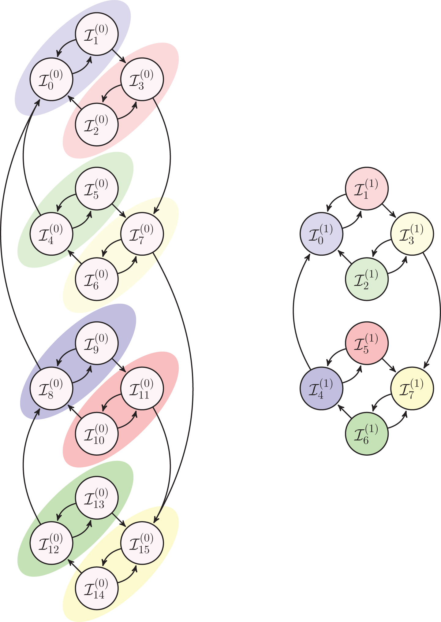
B. Implicit hierarchy

Here we demonstrate that intrinsic networks have a convenient multi-scale property where one can dismiss the smallest threshold from the framework and still preserve the structure. In order words, if we remove the directional change threshold δ₁ of an n-dimensional intrinsic network IN(n;{δ1,…,δn};W), the resulting structure is an n - 1-dimensional intrinsic network IN(n-1;{δ2,…,δn};Wˆ), whereas there is an explicit connection between transition matrices W and Wˆ, assuming the transitions on the network are modelled as first order Markov chain process.

Firstly, we introduce the concept of islands which are subsets of all possible states S={0,1,…,2n-1} the set of states of an n-dimensional intrinsic network IN(n;{δ1,…,δn};W). We define the k-th island as the following subset of states

(30)

Ik={s∈S:⌊s2⌋=k},

where ⌊· ⌋ denotes the floor function. In our cases, the k-th island equals Ik={2k,2k+1}. For instance, island I0 equals to subset {0, 1} or island I7 equals to subset {14, 15}. It is easy to notice that for an n-dimensional intrinsic network with 2ⁿ states, there are 2^n-1 islands. Note that we can again label the islands in numeric terms,

Ik=k,

creating a new set of states with numeric labels S(1)={0,…,2n-1-1}. Let us remark on the transitions among islands Ik. Given the numeric notation s = b₁ · 2⁰ + … + b_n · 2^n-1 for states of S, each state s(1)∈S(1) can be written in numeric notation as

s(1)=b2·20+…+bn·2n-2,

hence the transitions among islands are equivalent to occurrences of directional changes for thresholds δ₂, …, δ_n. In other words, transitions among islands are insensitive to changes in the market state related to first directional change thresholds δ₁, hence the resulting structure is an n - 1 dimensional intrinsic network IN(n-1;{δ2,…,δn},Wˆ). The probabilities of transition matrix Wˆ and its connection to transition matrix W is established later in this section. We refer to the presented method as state contraction.

Let us extend the concept of state contraction by defining islands of level 0, Ik(0) as the states of an n-dimensional intrinsic network

Ik(0)={k}, k=0,1,…,2n-1.

If S(0)={0,1,…,2n-1}={I0(0),…,I2n-1(0)} de-notes the states of n dimensional intrinsic network then we define islands of level 1, in notation Ik(1) as subsets

(31)

Ik(1)={I(0)∈S(0):⌊I(0)2⌋=k}

for k = 0, 1, …, 2^n-1 - 1. Using the aforementioned iterative process we can obtain islands of level j, in notation I(j), by applying the process of state contraction j times, hence we can then define an intrinsic network of level j + 1, IN(j+1) whereas the states space S(j+1) are defined as islands I(j+1), in other words S(j+1)={I0(j+1),…,I2n-j-1(j+1)}. In more general sense, we can define islands of level i as a subset of islands of level i - 1, i.e.

Il(i)={I(i-1)∈S(i-1):⌊I(i-1)2⌋=l}.

Having started with an intrinsic network with a total of 2ⁿ, the intrinsic network of level j + 1, IN(j+1) will have a total of 2^n-j states.

Figure 8 illustrates the process of state contraction, of 4-dimensional intrinsic network IN (4 ; {δ₁, …, δ₄} ; W) whereas the islands I0(0),…,I15(0) are contracted in the following manner

Ii(1)={I2i(0),I2i+1(0)}.

The coloured shading graphs islands, contracted states and the resulting new states of the three dimensional intrinsic network IN(3;{δ2,δ3,δ4};Wˆ).

Assuming the transitions on the intrinsic network are modelled as a first order Markov chain, there is an explicit connection between the transition matrix W of the n-dimensional intrinsic network and transition matrix Wˆ of the n - 1 dimensional intrinsic network obtained through the contraction process described above.

Let us assume that the current state of the network is Ik(i) and we are interested in finding the probability of transitioning to state Ij(i). Note that observing the process from viewpoint of islands of level (i - 1), the system can oscillate among states I2k(i-1) and I2k+1(i-1) arbitrarily many times before taking the transition that links the islands Ik(i) and Ij(i). Hence, the desired probability can be easily derived using the closed form of geometric series. The three distinct cases are presented bellow, with the proof in Appendix C,

for mod (k + j, 2) = 0

(32)

ℙ(Ik(i)→Ij(i)) =ℙ(I2k+1(i-1)→I2j+1(i-1))1-ℙ(I2k+1(i-1)→I2k(i-1))·ℙ(I2k(i-1)→I2k+1(i-1))

for mod (k + j, 2) = 1 and k > j

(33)

ℙ(Ik(i)→Ij(i)) =ℙ(I2k(i-1)→I2j(i-1))·ℙ(I2k+1(i-1)→I2k(i-1))1-ℙ(I2k(i-1)→I2k+1(i-1))·ℙ(I2k+1(i-1)→I2k(i-1))

for mod (k + j, 2) =1 and k < j

(34)

ℙ(Ik(i)→Ij(i))=ℙ(I2k+1(i-1)→I2j+1(i-1))·ℙ(I2k(i-1)→I2k+1(i-1))1-ℙ(I2k(i-1)→I2k+1(i-1))·ℙ(I2k+1(i-1)→I2k(i-1)).

C. State contraction probabilities

We demonstrate that assuming the transitions on the intrinsic network are modelled as a first order Markov Chain, there is an explicit connection between the transition matrix W of the n-dimensional intrinsic network and transition matrix Wˆ of the n - 1 dimensional intrinsic network obtained through the contraction process.

Let us assume that the current state of the network is Ik(i) and we are interested in finding the probability of transitioning to state Ij(i). Note that Island Ik(i) consists of states {I2k(i-1),I2k+1(i)}, while Island Ij(i) consists of state {I2j(i-1),I2j+1(i)}. For mod (k + j, 2) =0, from I2k+1(i-1) the system can directly transition to I2j+1(i-1) with probability ℙ(I2k+1(i-1)→I2j+1(i-1)). On the other hand, the system can oscillate once within Island Ik(i) before proceeding to Island Ij(i), i.e. transition from I2k+1(i-1) to I2k(i-1) and back to I2k+1(i-1), before transitioning to I2j+1(i), with probability

ℙ(I2k+1(i-1)→I2k(i-1))·ℙ(I2k(i-1)→I2k+1(i-1))·ℙ(I2k+1(i-1)→I2j+1(i-1)).

Likewise, oscillation within Island Ik(i) can occur k times, before proceeding to Island Ij(i), with probability,

(ℙ(I2k(i-1)→I2k+1(i-1))·ℙ(I2k+1(i-1)→I2k(i-1)))k·ℙ(I2k+1(i-1)→I2j+1(i-1)),

hence the probability to transition from Island Ik(i) to Island Ij(i) equals

(35)

ℙ(Ik(i)→Ij(i))=∑k=0∞(ℙ(I2k(i-1)→I2k+1(i-1))·ℙ(I2k+1(i-1)→I2k(i-1)))k·ℙ(I2k+1(i-1)→I2j+1(i-1))

(36)

=ℙ(I2k+1(i-1)→I2j+1(i-1))1-ℙ(I2k(i-1)→I2k+1(i-1))·ℙ(I2k+1(i-1)→I2k(i-1)).

For mod (k + j, 2) =1 and k > j, the system has to make an interim transition from I2k+1(i-1) to I2k(i-1), before transitioning from Island Ik(i) to Island Ij(i), with probability

ℙ(I2k+1(i-1)→I2k(i-1))·ℙ(I2k(i-1)→I2j(i-1)).

Likewise, as before the system can oscillate k times within Island Ik(i) before proceeding to Island Ij(i), with probability

ℙ(I2k+1(i-1)→I2k(i-1))·(ℙ(I2k(i-1)→I2k+1(i-1))·ℙ(I2k+1(i-1)→I2k(i-1)))k·ℙ(I2k(i-1)→I2j(i-1)),

hence the probability to transition from Island Ik(i) before to Island Ij(i) equals

(37)

ℙ(Ik(i)→Ij(i)) =∑k=0∞ℙ(I2k+1(i-1)→I2k(i-1))·(ℙ(I2k(i-1)→I2k+1(i-1)) ·ℙ(I2k+1(i-1)→I2k(i-1)))k·ℙ(I2k(i-1)→I2j(i-1))

(38)

=ℙ(I2k+1(i-1)→I2k(i-1))·ℙ(I2k(i-1)→I2j(i-1))1-ℙ(I2k(i-1)→I2k+1(i-1))·ℙ(I2k+1(i-1)→I2k(i-1)).

Similarly, it can be shown that for mod (k + j, 2) =1 and k < j, it can be shown

(39)

ℙ(Ik(i)→Ij(i)) =∑k=0∞ℙ(I2k(i-1)→I2k+1(i-1))·(ℙ(I2k(i-1)→I2k+1(i-1)) ·ℙ(I2k+1(i-1)→I2k(i-1)))k·ℙ(I2k+1(i-1)→I2j+1(i-1))

(40)

=ℙ(I2k(i-1)→I2k+1(i-1))·ℙ(I2k+1(i-1)→I2j+1(i-1))1-ℙ(I2k(i-1)→I2k+1(i-1))·ℙ(I2k+1(i-1)→I2k(i-1)).

D. Transition probability derivation

We demonstrate the derivation of the analytic expressions of transition probabilities presented in Section 5. Firstly, we prove the claim holds for 3-dimensional intrinsic network, let δ₁ < δ₂ < δ₃ denote the ordered directional change thresholds, IN(3;{δ1,δ2,δ3};W) 3-dimensional intrinsic network and IN(2;{δ2,δ3};Wˆ) the contracted intrinsic network. Since the contracted intrinsic network is 2-dimensional, it is know that

ℙ((1,0)→(1,1))=e-δ3-δ2δ2,

while the explicit analytic expression of transition probabilities between 3- and contracted 2-dimensional intrinsic network presented in Section 4 states that

e-δ3-δ2δ2=ℙ((1,1,0)→(1,1,1))1-(1-ℙ((1,1,0)→(1,1,1)))(1-e-δ2-δ1δ1)

and untangling the formula we find

(41)

ℙ((1,1,0)→(1,1,1))=e-δ3-δ2δ2e-δ2-δ1δ11-e-δ3-δ2δ2(1-e-δ2-δ1δ1)

yielding the desired expression. Let us assume that the claim holds for n-dimensional intrinsic network, and we will prove that the claim holds for n + 1. Let δ₁ < … < δ_n+1 denote the ordered directional change thresholds, IN(n+1;{δ1,…,δn+1};W) n + 1-dimensional intrinsic network and IN(n;{δ2,…,δn+1};Wˆ) the contracted intrinsic network. Since the contracted intrinsic network is n-dimensional, together with explicit analytic expression of transition probabilities between n + 1- and contracted n-dimensional intrinsic network presented in Section 4 states that

∏k=3n+1e-δk-δk-1δk-11-∑k=3n(1-e-δk-δk-1δk-1)∏j=k+1n+1e-δj-δj-1δj-1=ℙ((1,…,1,0)→(1,…,1,1))1-(1-ℙ((1,…,1,0)→(1,…,1,1)))(1-e-δ2-δ1δ1)

we find

(42)

ℙ((1,…,1,0)→(1,…,1,1))=

(43)

∏k=3n+1e-δk-δk-1δk-1·e-δ2-δ1δ11-∑k=3n(1-e-δk-δk-1δk-1)∏j=k+1n+1e-δj-δj-1δj-1-(1-e-δ2-δ1δ1)·∏k=3n+1e-δk-δk-1δk-1

obtaining the desired formula.

References

1	Bank of International Settlement. Triennial central bank survey foreign exchange turnover in april 2013, (2013) . Monetary and Economic Department.
2	Bauwens L., Hautsch N., (2009) . Modelling financial high frequency data using point processes. In Anderson T.G. and et al., editors, Handbook of financial time series, Springer, Berlin, pp. 953–976.
3	Brunnermeier K.M., (2009) . Deciphering the liquidity and credit crunch 2007–2008. Journal of Economic Perspectives 23: (1), 77–100.
4	Brunnermeier M.K., Nagel S., Pedersen L.H., (2008) . Carry trade and currency crashes, National Bureau of Economic Research Working Paper.
5	Chaboud A., Chiquoine B., Hjalmarsson E., Vega C., (2014) . Rise of the machines: Algorithmic trading in the foreign exchange market, (Forthcoming) Journal of Finance.
6	Clark P.K., (1973) . A subordinated stochastic process model with finite variance for speculative prices. Econometrica 41: , 125–156.
7	Cover T., Thomas J., (1991) . Elements of information theory. John Wiley & Sons, New York, NY, USA.
8	Dacorogna M.M., Gencay R., Müller U.A., Olsen R.B., Picet O.V., (2001) . An introduction to high-frequency finance. Academic Press, San Diego (CA).
9	Di Matteo T., Aste T., Dacorogna M.M., (2005) . Long term memories of developed and emerging markets: using the scaling analysis to characterize their stage of development. Journal of Banking and Finance 4: (4), 827–851.
10	Dorgan G. Snb losses 1.85 billion francs in just one day, 231 francs per inhabitant, 2012. SNBCHF.com.
11	Dukascopy., 2015. www.dukascopy, [Online; accessed 21-April-2015].
12	Fernandez F.A., (1999) . Liquidity risk, SIA Working Paper.
13	Gabrielsen A., Marzo M., Zagaglia P., (2011) . Measuring market liquidity: an introductory survey, MPRA Paper 35829, University Library of Munich.
14	Galluccio S., Caldarelli G., Marsili M., Zhang Y.C., (1997) . Scaling in currency exchange. Physica A 245: , 423–436.
15	Glattfelder J.B., Dupuis A., Olsen R.B., (2011) a. Patterns in high-frequency fx data: Discovery of 12 empirical scaling laws. Quantitative Finance 11: (4), 599–614.
16	Glattfelder J.B., Dupuis A., Olsen R.B., (2011) b. Patterns in high-frequency fx data: discovery of 12 empirical scaling laws. Quantitative Finance 11: (4), 599–614. doi: 10.1080/14697688.2010.481632. URL http://dx.doi.org/10.1080/14697688.2010.481632
17	Golub A., Chliamovitch G., Dupuis A., Chopard B., (2015) . Uncovering discrete nonlinear dependence with information theory. Entropy 17: (5), 2606. ISSN 1099-4300. doi: 10.3390/e17052606. URL http://www.mdpi.com/1099-4300/17/5/2606
18	Guillaume D.M., Pictet O.V.M., Müller U.A., Dacorogna M.M., (1995) . Unveiling non-linearities through time scale transformations, Olsen Working Paper.
19	Guillaume D.M., Dacorogna M.M., Dave R.R., Muller U.A., Olsen R.B., Pictet O.V., (1997) . From a bird’s eye to the microscope: A survey of new stylized facts of the intra-day foreign exchange markets. Finance and Stochastics 1: , 95–129.
20	Ito T., Hashimoto Y., (2006) . Intra-day seasonality in activities of the foreign exchange markets: Evidence from the electronic broking system. National Bureau of Economic Research Working Paper No. 12413.
21	Kavajecz K.A., Odders-White E.R., (2004) . Technical analysis and liquidity provision. The Review of Financial Studies 17: (4), 1043–1071.
22	LeBaron B., (1994) . Chaos and nonlinear forecastability in economics and nance. Philosophical Transactions: Physical Sciences and Engineering 348: (1688), 397–404. ISSN 09628428. URL http://www.jstor.org/stable/54216
23	Mandelbrot B.B., (1963) . The variaton of certain speculative prices. The Journal of Business 36: , 394–419.
24	Mandelbrot B.B., Taylor H.W., (1967) . On the distribution of stock price differences. Operations Research 15: , 1057–1062.
25	Müller U.A., Dacorogna M.M., Olsen R.B., Pictet O.V., Schwarz M.M., Morgenegg C., (1990) . Statistical study of foreign exchange rates, empirical evidence of a price change scaling law and intraday analysis. Journal of Banking and Finance 14: , 1189–1208.
26	Oanda. (2015) . www.oanda.com. “[Online; accessed 21-April-2015]”.
27	Pfister H.D., Soriaga J.B., Siegel P.H., (2001) . On the achievable information rates of finite state isi channels. In Kurlander D., Brown M. and Rao R., editors, Proc IEEE Globecom, ACMPress, pp. 41–50.
28	Poon S.-H., Granger C.W., (2003) . Forecasting volatility in nancial markets: A review. Journal of Economic Literature 41(2), 478–539. doi: 10.1257/002205103765762743. URL http://www.aeaweb.org/articles.php?doi=10.1257/002205103765762743
29	Sarr A., Lybek T., (2002) . Measuring liquidity in financial market, IMF Working Paper No. 02/232.
30	Schmidt A., (2011) . Ecology of the modern institutional spot fx: The ebs market in 2011. Technical report, Electronic Broking Service.
31	von WyssR., (2004) . Measuring and Predicting Liquidity in the Stock Market. PhD thesis.

Figures and Tables

Fig.1

Price evolution example over a week-end. Directional change events (squares) act as natural dissection points, decomposing a total-price move between two extremal price levels (bullets) into so-called directional-change (solid lines) and overshoot (dashed lines) sections. Time scales depict physical time ticking evenly across different price curve activity regimes, whereas intrinsic time triggers only at directional change events, independent of the notion of physical time. The time period where the exchange rate does not change corresponds to the weekend.

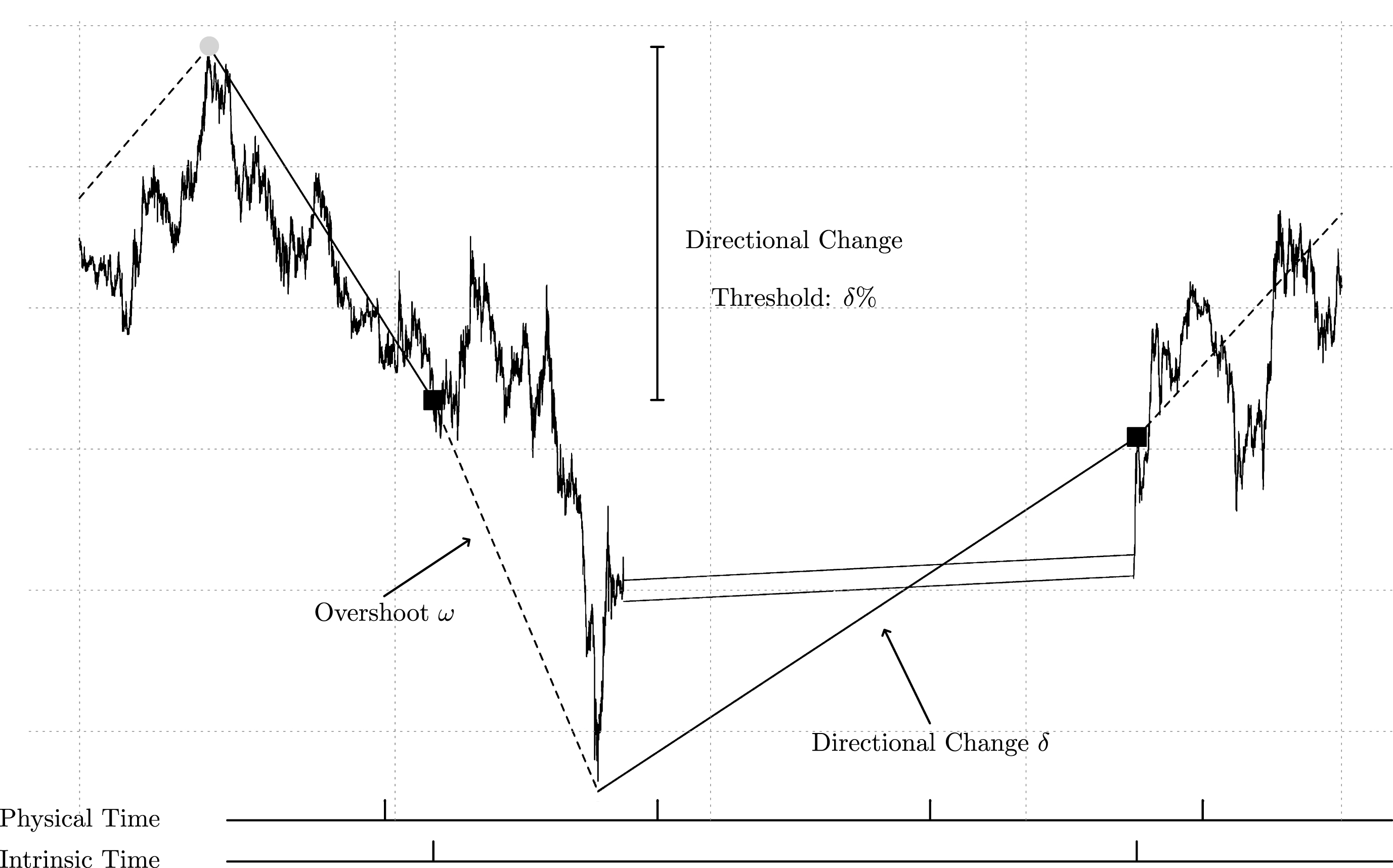
Fig.2

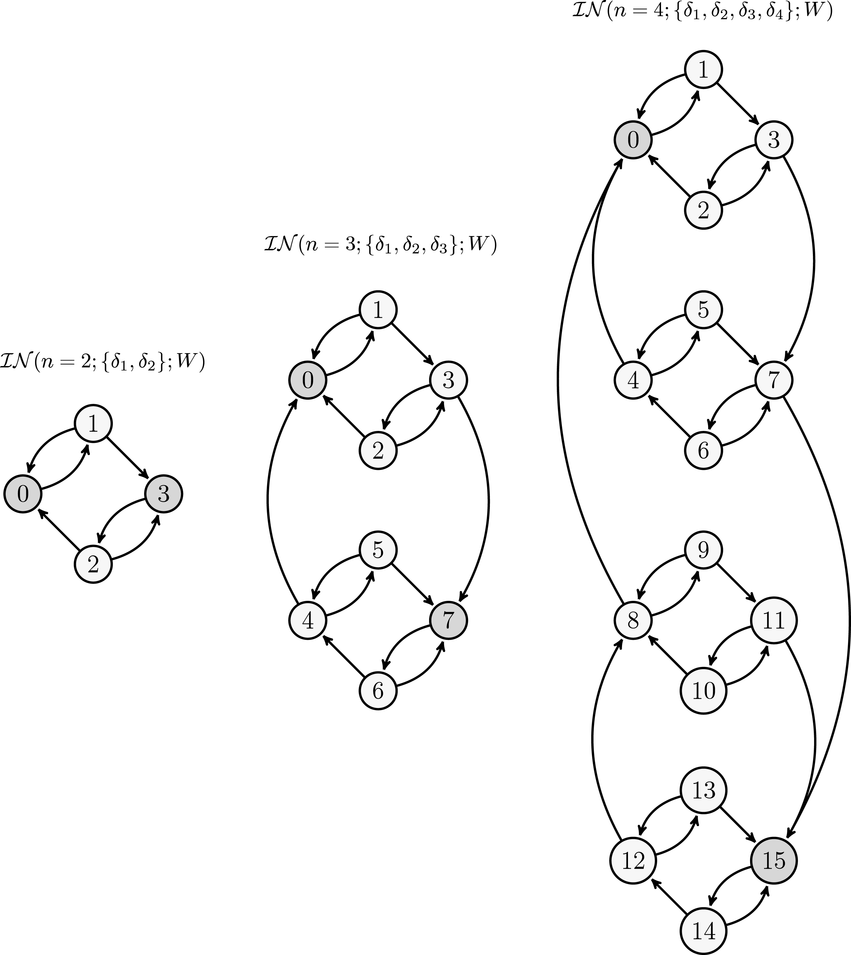
From left to right: 2-, 3- and 4-dimensional intrinsic networks IN, where transitions between states s are represented. Shaded nodes represent blind-spots. Each transition is associated with a probability.

Fig.3

Example of transitions on 2-dimensional intrinsic network for a time series. Transitions are coloured and depicted on the graph.

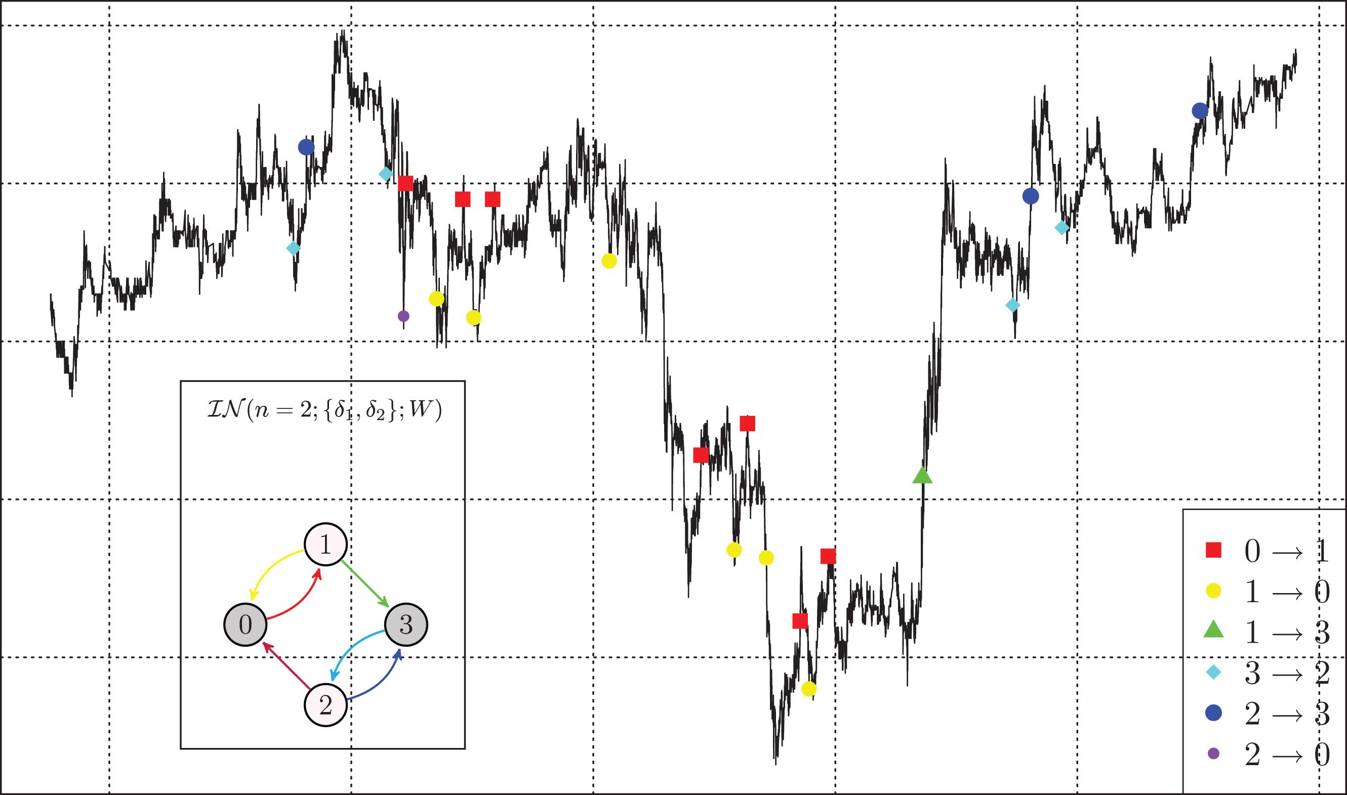
Fig.4

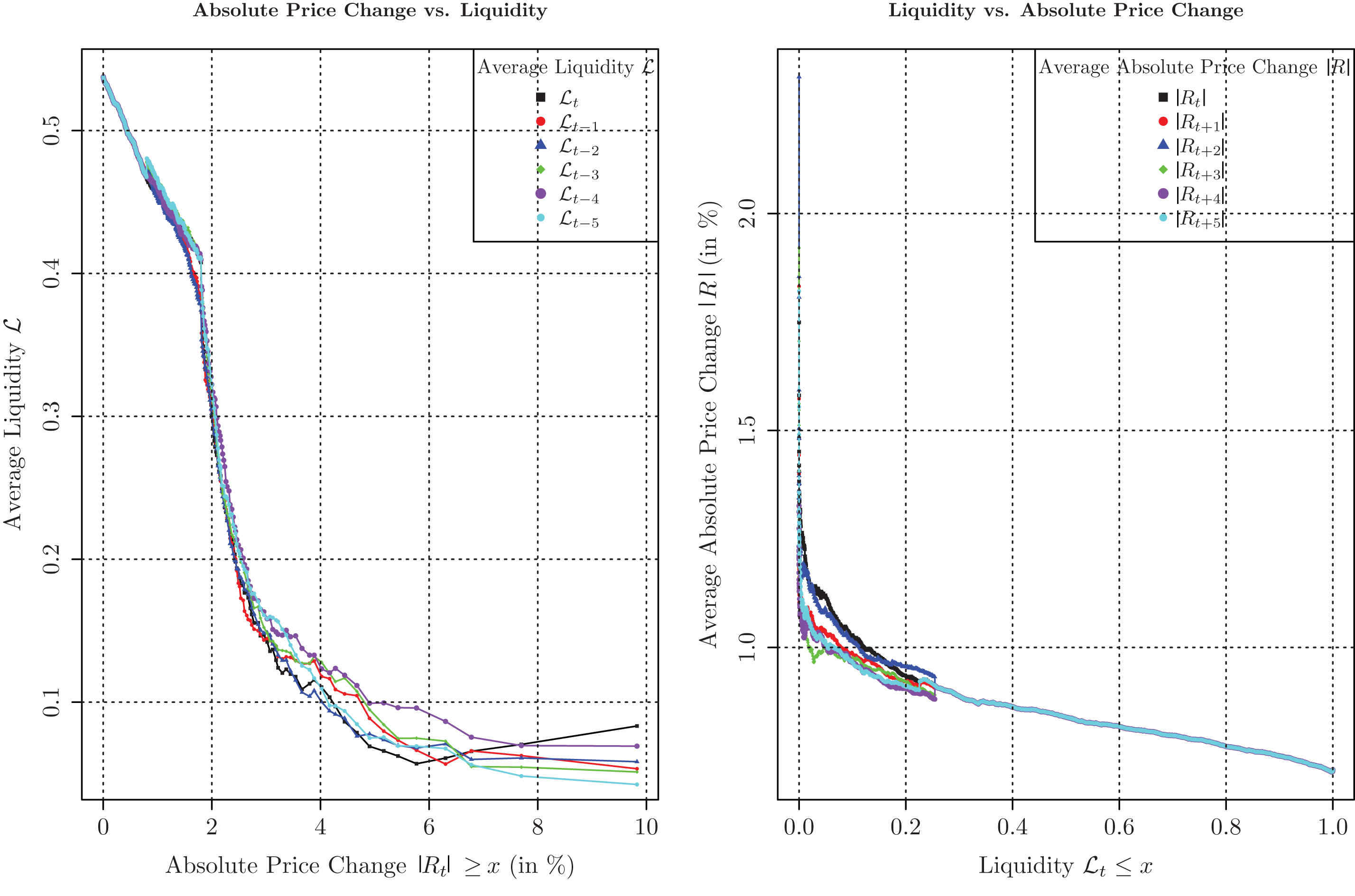
The left graph shows the relationship between absolute daily price changes larger than x and average liquidity 〈Lt-k〉(x), for up to 5 days before the occurrence of the price change. The right graph shows the relationship between liquidity 〈Lt-k〉(x) smaller than x and average absolute daily price changes, for up to 5 days after the occurrence of the price change.

Fig.5

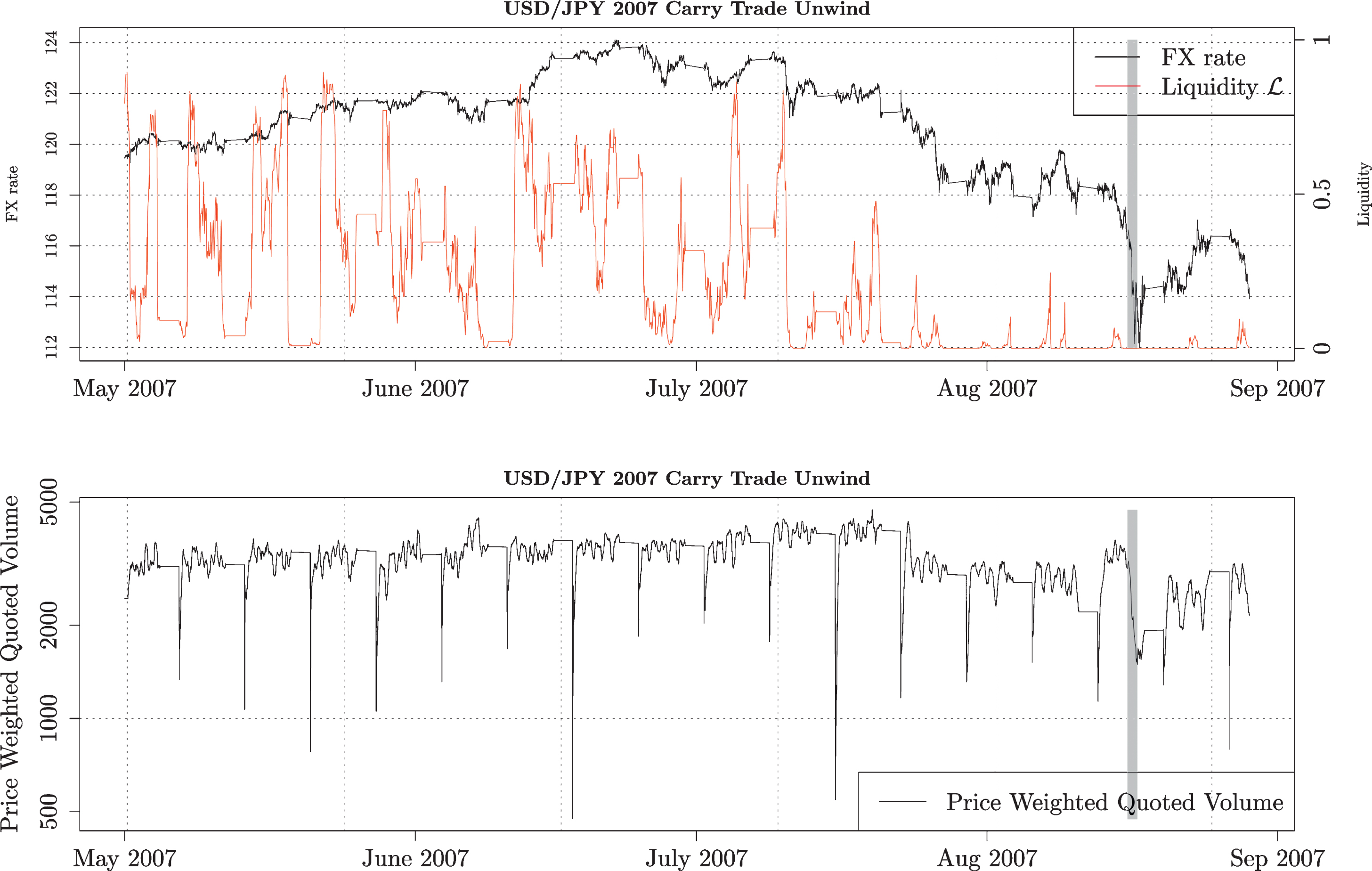
The upper graph shows tick-by-tick USD/JPY exchange rate (left axis) and the corresponding one minute liquidity measurement L (right axis) around the period of August 2007 carry trade unwind. The lower graph shows average price weighted quoted volume over a 24 hour period, graphed every minute. The shaded area marks August 16th 2007, day of the carry trade unwind, resulting in a 6% drop.

Fig.6

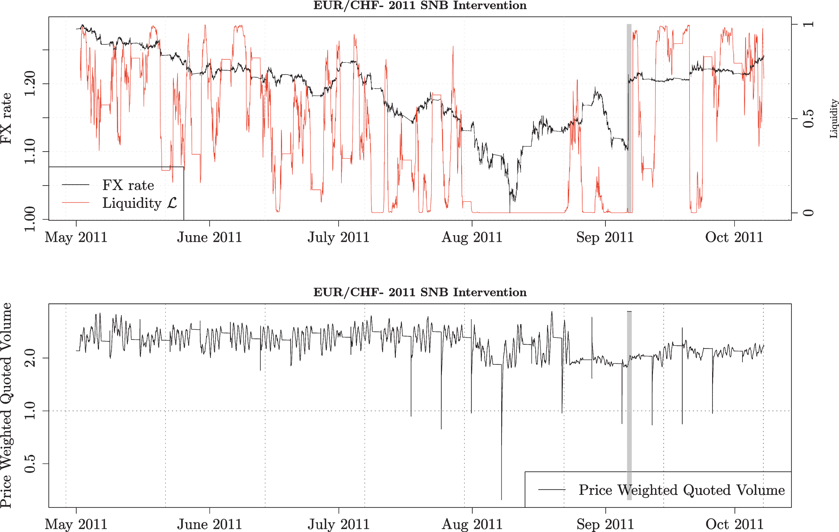
The upper graph shows tick-by-tick EUR/CHF exchange rate (left axis) and the corresponding one minute liquidity L (right axis) in the months of Swiss National Bank intervention, setting the floor of 1.20 on EUR/CHF. The lower graph shows average price weighted quoted volume over a 24 hour period, graphed every minute. The shaded area marks September 6th 2011, day of SNB intervention.

Fig.7

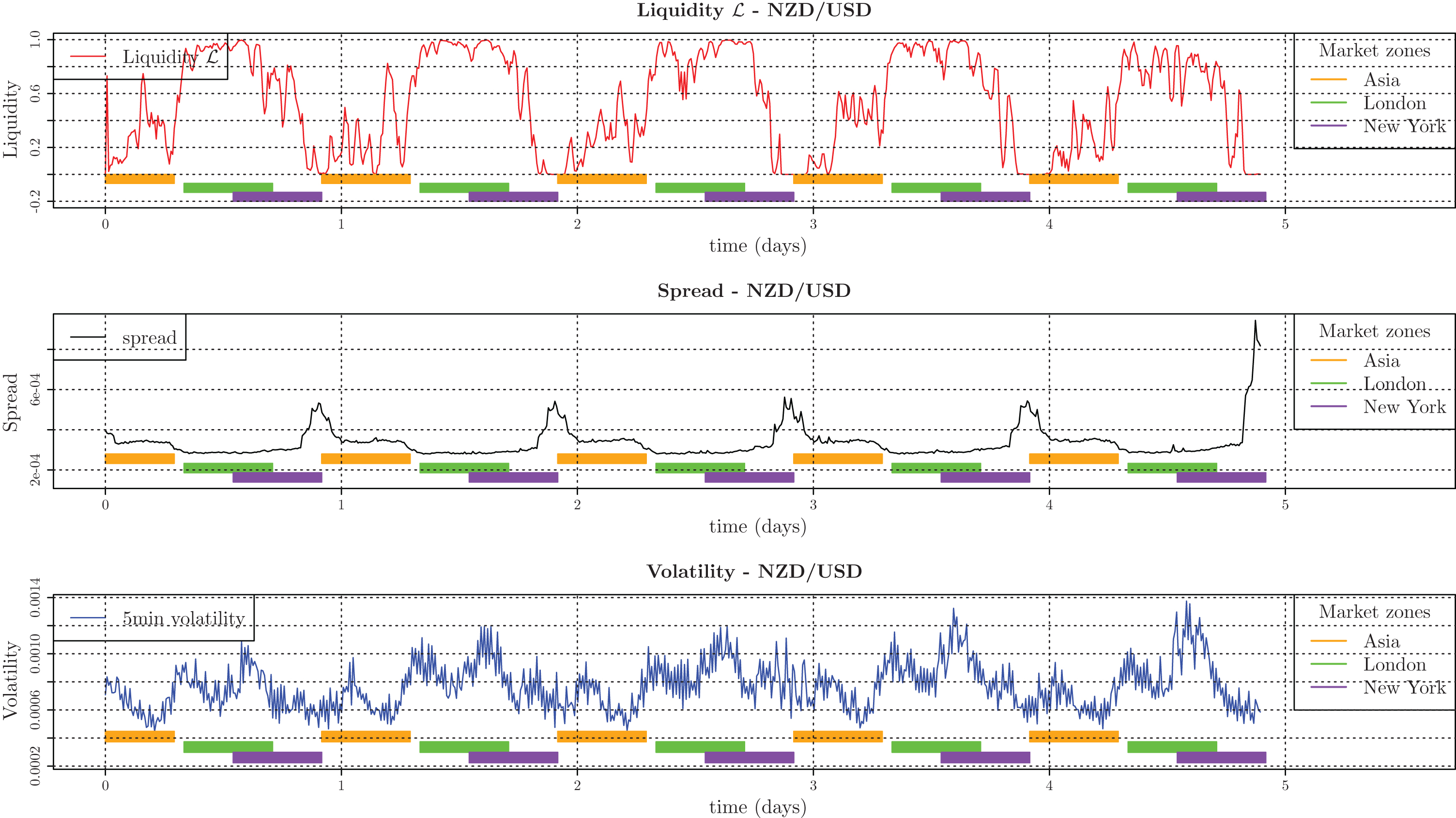
The graph shows intra-week seasonality pattern for liquidity L, spread and volatility, for NZD/USD. Market zones are denoted as follows: Asia - orange, London - green, New York - purple.

Fig.8

Illustration of the contraction procedure of a 4-dimensional intrinsic network IN(4;{δ1,δ2,δ3,δ4};W) to a 3-dimensional intrinsic network IN(3;{δ2,δ3,δ4};Wˆ), whereas coloured shading graphs islands, contracted states and the resulting new states.