Super-resolution of diffusion-weighted images using space-customized learning model

Zhao, Xitong; Wen, Zhijie

doi:10.3233/THC-248037

Super-resolution of diffusion-weighted images using space-customized learning model

Article type: Research Article

Affiliations: Department of Mathematics, College of Sciences, Shanghai University, Shanghai, China

Correspondence: [*] Corresponding author: Zhijie Wen, Shanghai University, 99 Shangda Road, Baoshan District, Shanghai, China. E-mail: [email protected].

Keywords: CNN, diffusion-weighted imaging, graph convolution, super-resolution

DOI: 10.3233/THC-248037

Journal: Technology and Health Care, vol. 32, no. S1, pp. 423-435, 2024

Published: 31 May 2024

Get PDF

Abstract

BACKGROUND:

Diffusion-weighted imaging (DWI) is a noninvasive method used for investigating the microstructural properties of the brain. However, a tradeoff exists between resolution and scanning time in clinical practice. Super-resolution has been employed to enhance spatial resolution in natural images, but its application on high-dimensional and non-Euclidean DWI remains challenging.

OBJECTIVE:

This study aimed to develop an end-to-end deep learning network for enhancing the spatial resolution of DWI through post-processing.

METHODS:

We proposed a space-customized deep learning approach that leveraged convolutional neural networks (CNNs) for the grid structural domain (x-space) and graph CNNs (GCNNs) for the diffusion gradient domain (q-space). Moreover, we represented the output of CNN as a graph using correlations defined by a Gaussian kernel in q-space to bridge the gap between CNN and GCNN feature formats.

RESULTS:

Our model was evaluated on the Human Connectome Project, demonstrating the effective improvement of DWI quality using our proposed method. Extended experiments also highlighted its advantages in downstream tasks.

CONCLUSION:

The hybrid convolutional neural network exhibited distinct advantages in enhancing the spatial resolution of DWI scans for the feature learning of heterogeneous spatial data.

1.Introduction

As the only noninvasive technique for in vivo examination of white matter tracts, diffusion-weighted imaging (DWI) plays a pivotal role in brain research [1]. However, DWI often encounters challenges in terms of quality due to the tradeoff between resolution, signal-to-noise ratio (SNR), and scanning time [2, 3]. For instance, acquiring higher-resolution DWI scans undesirably prolongs scanning time and lowers SNR. Conversely, low-resolution (LR) DWI can result in significant partial-volume effects and introduce bias into subsequent processing steps, such as diffusion tensor fitting, fiber tractography, and brain connectome construction. The demand for higher imaging spatial and angular resolutions has increased with the advancement of the model’s capability to depict tissue microstructure. The duration of magnetic resonance imaging (MRI) scans varies depending on several factors and typically ranges from 10 min to more than an hour. DWI necessitates longer scan times due to the requirement for a larger number of sequences. Patients must maintain a fixed posture and remain still during scanning to ensure data acquisition quality, which can be particularly challenging for infants. Despite continuous progress in DWI, it has consistently faced the predicament of limited promotion and application in clinical practice. Hence, addressing the urgent technical issue of meeting both high-quality imaging and high-efficiency requirements for the clinical implementation of diffusion MRI has become imperative. Super-resolution (SR) techniques can be employed to enhance the spatial resolution of DWI scans. In fact, SR has been a longstanding topic within the MRI community with various algorithms already developed for the SR of MRI scans [4, 5, 6, 7, 8, 9, 10, 11]. All of these methods aim to map LR images to their high-resolution (HR) counterparts using voxel correlations within an image or between different slice orientations.

The process of image acquisition can be perceived as a form of degradation, which can be mathematically represented as Y=f⁢(X)+N, where X represents the original HR image, Y is the observed LR image, f denotes the down-sampling function, and N represents the noise. Recovering X from Y poses a challenging inverse problem [12, 13]. SR techniques can be categorized into multi-image-based SR (MISR) and single-image-based SR (SISR) depending on the number of input images used. MISR uses multiple LR images to reconstruct an HR image. For instance, Greenspan and Scherrer acquired several LR DWI scans using anisotropic orthogonal scanning and then reconstructed the HR DWI scans based on them after making necessary corrections [2, 9]. Compared with MISR, SISR requires only a single LR image to predict its corresponding HR counterpart, making it more practical for clinical applications [14].

The DWI scans exist within a combined 6D domain, encompassing both the x-space (spatial domain) and q-space (diffusion wave-vector domain). Within the x-space, diffusion signals are structured as a collection of volumes with a 3D grid arrangement. Tanno et al. assessed the uncertainty of CNNs for Bayesian quality transfer of DWI scans to enhance their spatial resolution [15]. They introduced generative adversarial networks to augment the spatial resolution of DWI scans. Additionally, attempts were made to leverage joint features from both x-space and q-space, represented by a graph, to learn missing information during longitudinal brain studies in infant [3]. Furthermore, efforts were made to optimize memory and computation costs to reduce model parameter capacity while ensuring efficient operation for deeper image quality transfer tasks [16]. Finally, SR generative adversarial network, enhanced deep SR network, and bicubic interpolation were employed in conjunction with each other to generate HR DWI scans for breast tumor detection [17, 18].

The DWI signal is associated with both the three-dimensional (3D) Euclidean space (x-space) and the diffusion gradient angle space (q-space). Its heterogeneous and high-dimensional characteristics pose challenges for effective learning using convolutional neural networks (CNNs). Although significant research progress has been made in DWI SR technology using deep learning (DL), existing methods primarily focus on feature learning in x-space and do not fully exploit the correlation between diffusion gradient directions in q-space. Existing models for image SR in DWI can be broadly classified into two groups. The first group primarily focuses on increasing spatial resolution without considering the impact of q-space, as demonstrated by Alexander et al. [11] and Tanno et al. [15]. The second group pays more attention to a unified framework by integrating both x-space and q-space with compromises induced by heterogeneous domain fusion, as proposed by Chen et al. [3]. For overcoming these limitations, we proposed a two-stage domain-directed (TSDD) learning network that fully exploited correlations in both x-space and q-space to enhance the spatial resolution of DWI scans. In this study, “Domain Directed” refers to the guiding convolution type based on the structure inherent to each domain. Specifically, we relied on CNNs for effective perception in x-space and on graph CNNs (GCNNs) for exploiting correlations in q-space. We designed a cascaded hybrid neural network comprising CNNs and GCNNs to address the aforementioned drawbacks. First, a residual CNN sub-network predicted coarse SR in the x-space. Subsequently, GCNN refined this coarse SR in q-space. Compared with the existing models that operated solely within specific domains, our approach leveraged the strengths of both CNNs in grid-structure domains and GCNNs in non-Euclidean domains. Furthermore, serving as a post-processing method, the approach was independent of scanning protocols. We evaluated our method using data from the Human Connectome Project (HCP), demonstrating satisfactory performance achieved by TSDD.

The structure of our manuscript is outlined as follows. Section 2 provides a comprehensive description of our network architecture. In Section 3, we present the datasets and discuss the obtained results. Section 4 delves into insightful discussions. Finally, in Section 5, we conclude our work.

2.Materials and methods

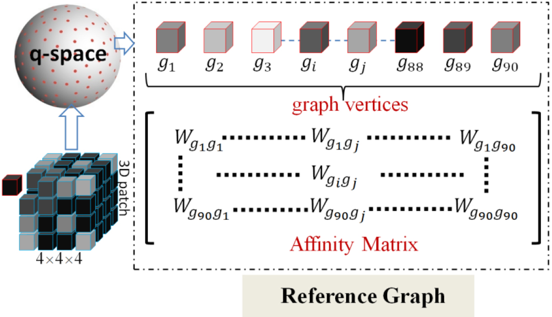
Existing studies have demonstrated the exceptional learning performance of CNN in domains characterized by a grid structure. However, the effectiveness of CNN is limited when applied to non-Euclidean spaces [19]. We proposed an end-to-end heterogeneous deep neural network that combined both CNN and GCNN in the case of DWI scans where 3D volumes were sampled from q-space (a non-Euclidean and wave-vector domain). Our approach involved using CNN to initially predict HR DWI scans in x-space for each volume, followed by refining these predictions using GCNN to exploit the correlations among diffusion gradients in q-space. The application of GCNN followed ChebNet [19], which was based on graph spectrum analysis [20]. The output of CNN needed to be formatted accordingly to meet the requirements of GCNN. For this purpose, we predefined a fixed graph as the reference for graph learning in this study. The construction details of the reference graph are visualized in Fig. 1 and discussed in Section 2.1. Additionally, Section 2.2 provides an introduction to GCNN, whereas Section 2.3 presents a summary and discussion of our network architecture depicted in Fig. 2. Finally, Section 2.4 outlines the loss function employed for this task.

Figure 1.

Illustration of reference graph construction. The 3D patch represents the coarse SR prediction. The reference graph was composed of a graph node set and an adjacency matrix. The graph node set consisted of all of the diffusion gradient directions. The adjacency matrix could be induced from affinity, which was a symmetric matrix that denoted the connection weight between any two diffusion gradient directions.

2.1Reference graph

In the first stage, a CNN-based sub-network was used to predict a coarse DWI SR in the x-space. However, the coarse SR obtained could not be directly fed into the subsequent GCNN-based sub-network due to the inconsistent data format. Graph-structured samples are essential for GCNN. Therefore, we needed to bridge the format gap and make training feasible in our two-stage network with hybrid convolutions. To achieve this goal, we constructed a reference graph in q-space to leverage correlations among diffusions. This reference graph served as an indispensable component for graph convolution operations in our experiments. The details of reference graph construction are illustrated in Fig. 1.

(1)

𝑾i⁢j=e1-(gi→⋅gj→)2-𝝈

where i, j∈[1,…,𝐍] are the indices of diffusion gradient directions, 𝒈i→⋅𝒈j→ is the dot product, and σ is the bandwidth of the Gaussian kernel. As illustrated in Fig. 1, diffusion signals of each voxel in the coarse SR 3D patch were arranged in order as the graph signal. Affinity matrix is a symmetric positive definite matrix, and 𝑾i⁢j is the quantified correlation of any two diffusion gradient directions in the q-space. From the affinity matrix, a weighted adjacency matrix could be easily induced by setting the main diagonal elements with 0. The evaluation of our model is currently limited to single-shell DWI scans (b value = 1000) due to computational resource constraints. However, we plan to extend it to multi-shell DWI SR in the future.

2.2Graph CNN

In the last decade, DL has demonstrated exceptional performance across various applications. Particularly, CNNs and recurrent neural networks have achieved state-of-the-art results in computer vision and speech recognition tasks. Generally, CNNs are employed for feature extraction from 2D or 3D grid-structured data. However, they cannot be directly applied to high-dimensional or non-Euclidean datasets such as citations and social networks. DWI data possess both high-dimensional and non-Euclidean characteristics due to the dependence of their voxel values on spatial location and diffusion wave-vector. Conventional CNN models also exhibit limited effectiveness when applied to DWI data.

Many approaches have been proposed for the application of DL to non-Euclidean data, including those by Bronstein et al., Lee et al., and Li et al. [21, 22, 23]. Among these, GCNN stands out as a convolutional model based on graph spectrum, which was initially introduced by Bruna et al. [20]. Compared with CNNs, GCNNs offer a more versatile learning framework that leverages frequency domain multiplication to define graph convolutions and allows for the definition of graph filters as follows:

(2)

y=gθ⁢(𝑳)⁢x=gθ⁢(U⁢𝚲⁢UT)⁢x=U⁢gθ⁢(𝚲)⁢UT⁢x

where 𝑳 is the Laplacian matrix of the graph, U is graph Fourier transformation (GFT), and UT is inverse GFT. gθ⁢(𝚲) is a nonparametric filter defined as follows:

(3)

gθ⁢(𝚲)=𝑑𝑖𝑎𝑔⁢(θ)

where θ∈Rn is a vector of Fourier coefficients. However, it is not a localized filter in space. Therefore, it is localized using Kth order polynomials of the Laplacian Henaff et al. [24]. The localized graph filter is defined as follows:

(4)

gθ⁢(Λ)=∑k=0K-1θk⁢𝚲k

where θ∈Rk is a vector of polynomial coefficients. To accelerate graph filtering, Defferrard et al. [19] and A et al. [25] introduced the use of the Chebyshev polynomial, leading to the following revision of the graph filter:

(5)

gθ⁢(Λ)=∑k=0K-1θk⁢Tk⁢(𝚲~)

where Tk⁢(Λ~)∈Rn×n is the Chebyshev polynomial of order k evaluated at 𝚲~=2⁢Λ/𝝀max-In, 𝚲=𝐷𝑖𝑎𝑔⁢([λ0,…,λn-1])∈𝑹n×n denotes the associated ordered real non-negative eigenvalues {λl}l=0n-1, and 𝝀max is the maximum eigenvalue of the graph Laplacian matrix, which is defined as 𝑳=𝑫-𝑾∈𝑹n×n, where 𝑫∈𝑹n×n is the diagonal degree matrix with 𝑫i⁢j=∑j𝑾i⁢j. The filtering operation is written as y=gθ⁢(L)⁢x=∑k=0K-1θk⁢Tk⁢(L~)⁢x, where Tk⁢(L~)⁢x∈𝑹n×n is the Chebyshev polynomial of order k evaluated at the scaled Laplacian. According to the recurrence relation x¯k=2⁢L~⁢x¯k-1-x¯k-2 with x¯k=Tk⁢(L~)⁢x∈Rn, x¯0 and x¯1=L~x. The filtering operation is defined as y=gθ⁢(L)⁢x=[x¯0,…,x¯k-1]⁢θ.

GCNN has displayed outstanding performance in some studies. For instance, Kipf and Welling proposed a semi-supervised learning network based on GCNN for citation network classification [26]. Ktena et al. used GCNN to examine the difference between two functional brain networks [27]. The correlations in q-space were fully exploited in this task based on GCNN to improve the performance of DWI SR. Section 2.3 explains in detail how to build a hybrid neural network, and Section 2.4 describes how to train a hybrid neural network in the DWI SR task.

2.3TSDD neural network

As previously mentioned, DWI data exist in a 6D space, consisting of three dimensions for spatial space and three dimensions for diffusion directions. Each diffusion direction has a DWI scan organized as a volume with a 3D grid structure. Leveraging this prior structural information is advantageous for SR performance. Given the significant advantages of CNNs in learning tasks involving 2D or 3D data, we first employed them for coarse SR prediction. Additionally, we proposed using correlations in diffusion gradients to enhance SR performance because the diffusion signal was influenced by not only spatial position but also diffusion gradient direction.

We referred to our proposed SR method as the TSDD neural network. In the first stage, we developed a 3D version of dense convolutional networks (DenseNet [28]) to generate a coarse SR prediction solely based on the 3D DWI scans. Subsequently, in the second stage, we transformed this coarse prediction into a graph using the approach described in Section 2.1 and enhanced it through GCNN refinement. Thus, we effectively leveraged the strengths of CNNs and GCNNs across distinct data domains for accomplishing the DWI SR task.

Figure 2.

Architecture of our proposed two-stage domain-directed network to reconstruct HR DWI scans. The first stage included the coarse SR DWI scans (CSR) based on CNN in x-space. The second stage included the refinement using GCNN in q-space.

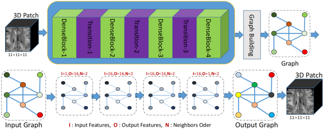
As shown in Fig. 2, our network consisted of two sub-networks: dense CNN and graph CNN. The input of our network was the LR DWI scans, whereas the target output was the SR DWI scans. The whole pipeline could be formulated as follows:

(6)

IH=Fq⁢(Fx⁢(IL))

where IL is the LR DWI, IH is the HR DWI scan, Fx is the learning module in the x-space, and Fq is the learning module in the q-space.

DenseNet has proven to be highly effective in image SR tasks because it promotes feature reuse and alleviates the vanishing gradient problem that can plague deep networks [29, 30, 31]. The output of DenseNet is a coarse SR prediction, which is enhanced in the x-space with a 3D grid structure. The signals of each voxel at all diffusion gradients were organized as a vector, as discussed in Section 2.1. Then, leveraging the reference graph illustrated in Fig. 1, the CSR was represented as a graph and inputted into the sub-network based on GCNN.

The input of GCNN consisted of two parts: graph signal and reference graph. The representation of the graph signal and reference graph is shown in Fig. 1. The specific generation process has been described in detail in Section 2.1. The graph CNN in this study was based on ChebNet [19]. The specific convolution operation definition has been explained in Section 2.2. The graph convolutional layer primarily involved two parameters: the order of the Chebyshev polynomial and the number of filters, also known as channels. These parameters collectively determined the capacity of network parameters. The order of the Chebyshev polynomial determined both the number of parameters in the graph convolution filter and its neighborhood range within the graph. The experimental results demonstrated that an optimal outcome could be achieved when setting the order to 2, with minimal impact on performance, by increasing it further. In this study, all graph convolution filters in GCNN were set to order 2. For our experiments, we configured the number of channels for each graph convolutional layer as follows: 1 channel for input graphs, 64 channels for middle layers, and 1 channel for the final layer. Following this output graph stage, three additional convolutional layers similar to those used at the inception of CNN were employed to strike a balance between smoothing and sharpening.

2.4Loss function

The DWI SR in this task was considered as a regression procedure from LR to HR. Similar to most regression networks, the mean square error (MSE) was used as an objective function in both CNN- and GCNN-based sub-networks. The details of the MSE loss was defined as follows:

(7)

𝐿𝑜𝑠𝑠𝑚𝑠𝑒=∑i=1n∑j=1N(V^i⁢j-Vi⁢j)2𝒏*𝑵

where 𝒏 is the number of voxels in the 3D patch, 𝑵 is the number of diffusion gradient directions, 𝒊 is the index of voxels, 𝒋 is the index of diffusion gradient direction, V^i⁢j is the prediction of the voxel value of the 𝒊th voxel in the 3D patch along 𝒋th diffusion gradient direction, and Vi⁢j is the ground truth.

According to the graph spectral theory, edge connections between nodes in a graph can be expressed as a Laplacian matrix. To evaluate the similarity between the predicted and target graphs, we defined Laplacian loss as follows:

(8)

𝐿𝑜𝑠𝑠𝑙𝑎𝑝=∑i=1n(L×V^i-L×Vi)2n

where n is the number of voxels in the 3D patch, V^i is the graph signal of 𝒊th voxel in the predicted HR 3D patch, 𝒱i is the graph signal of the corresponding voxel in the target HR 3D patch, and 𝑳 is the Laplacian matrix of the graph. 𝑳×𝑽 can be viewed as the second-derivative transformation on the graph, representing the projection of voxel signal values onto the graph. Our training consisted of the following two steps to ensure a stable error gradient backpropagation for updating parameters in two heterogeneous convolution sub-networks (CNN and GCNN). In the first step, we just updated the parameters of CNN sub-networks. The total loss was defined as follows:

(9)

𝐿𝑜𝑠𝑠𝑡𝑜𝑡𝑎𝑙=𝐿𝑜𝑠𝑠𝑚𝑠𝑒+λ⋅∑ω¯i⁢j2

where λ⋅∑ω¯i⁢j2 is a regular parameter with coefficient λ= 1e-8 and ω¯i⁢j are parameters in the CNN sub-network. In the second step, the parameters in the CNN component were fixed; only the parameters in the GCNN sub-network were updated. The total loss was defined as follows:

(10)

𝐿𝑜𝑠𝑠𝑡𝑜𝑡𝑎𝑙=α⋅𝐿𝑜𝑠𝑠𝑚𝑠𝑒+β⋅𝐿𝑜𝑠𝑠𝑙𝑎𝑝+λ⋅∑ω¯i⁢j2

where α= 0.5 and β= 0.5 are weights for 𝐿𝑜𝑠𝑠𝑚𝑠𝑒 and 𝐿𝑜𝑠𝑠𝑙𝑎𝑝, ∑ω¯i⁢j2 is a regular parameter with coefficient λ= 1e - 8, and ω¯i⁢j are parameters in the GCNN sub-network.

3.Experiments

3.1Data

The actual brain diffusion MRI data used in this study were acquired by Washington University in Saint Louis and the University of Minnesota [32], and downloaded from the HCP. Scanning was performed on a Siemens 3T Skyra scanner using a 2D spin-echo single-shot multi-band EPI sequence with a multi-band factor of 3 and a monopolar gradient pulse. The spatial resolution was set to 1.25 mm isotropic, with TR = 5500 ms, TE = 89.50 ms, and a b value of 1000 s/mm². Besides the acquisition of 6 b0 images, 90 diffusion sampling directions were detected. The preprocessed data underwent correction for eddy current and susceptibility artifacts as described by Andersson et al. and Sotiropoulos [33, 34, 35]. The DWI scans were normalized to values between 0 and 1 by dividing them with the average b0 image intensity. LR DWI scans were obtained through down-sampling using linear interpolation from real HR DWI scans with a scale factor of two. We randomly selected 25 subjects from the HCP dataset, which were roughly divided into training set (20 subjects), validation set (2 subjects), and test set (3 subjects) according to an approximate ratio of 8:1:1, respectively. For each volume, we extracted 3D voxel patches with a fixed size and an offset of four units along each dimension. We maintained a consistent offset value of two units between adjacent patches within the scan volume of each subject. Each subject contributed approximately 30,000 non-background or non-zero-filled voxel patches, resulting in an estimated size for our training dataset of about 600,000 samples.

3.2Training setting

The Adam optimizer was employed to train our model, with an initial learning rate of 10-4 and a decay frequency of once every 5000 iterations. Other training settings were as follows: a batch size of 20 and a maximum epoch set to 300. Additionally, we used a nonzero-ratio of 0.1 to discard voxel patches containing excessive zeros. Our network implementation was based on the TensorFlow 1.9 framework. The training process took approximately 12 h using a single GTX 2080Ti GPU.

3.3Evaluation metrics

The computation of three quantitative metrics, such as MSE, peak signal-to-noise ratio (PSNR), and structural similarity (SSIM), was conducted as proposed previously [36]. The mathematical definitions for MSE, PSNR, and SSIM are presented in Eqs (11), (12), and (13), respectively. In this study, we solely evaluated our model using single-shell data while reserving the evaluation on multi-shell data for future investigation. MSE is defined as follows:

(11)

𝑆𝐸=1N×H×W×D⁢∑g=0N-1∑x=0H-1∑y=0W-1∑z=0D-1(V^g,x,y,z-Vg,x,y,z)2

where H, W, and D are the height, width, and depth of a 3D voxel patch, respectively, N is the number of diffusion gradient directions, V^g,x,y,z is the predicted signal value of the location (x,y,z) in the 3D voxel patch along the diffusion gradient direction g, and Vg,x,y,z is the ground truth. PSNR is defined as follows:

(12)

𝑃𝑆𝑁𝑅=10×log10⁡𝑀𝑎𝑥2𝑀𝑆𝐸

where Max denotes the maximum diffusion value. In our experiment, DWI data were normalized to the value range of (0 1); thus, Max was 1. SSIM is defined as follows:

(13)

𝑆𝑆𝐼𝑀=(2⁢μS⁢μH+C1)⁢(2⁢σ𝑆𝐻+C2)(μS2+μH2+C1)⁢(σS2+σH2+C2)

where μS and μH are the mean values of the predicted and ground-truth HR DWI scans, respectively, whereas 𝝈x and A𝝈y are the standard deviation of the predicted and ground-truth HR DWI scans, respectively, and 𝝈S and 𝝈H are the covariance. C1 and C2 are constants.

Figure 3.

Reconstructed HR DWI scans (first row) and the corresponding FA images (second row). The first column represents the input low-resolution DWI scan.

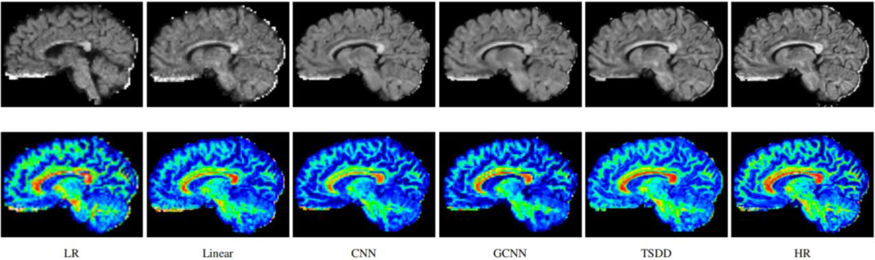
Figure 4.

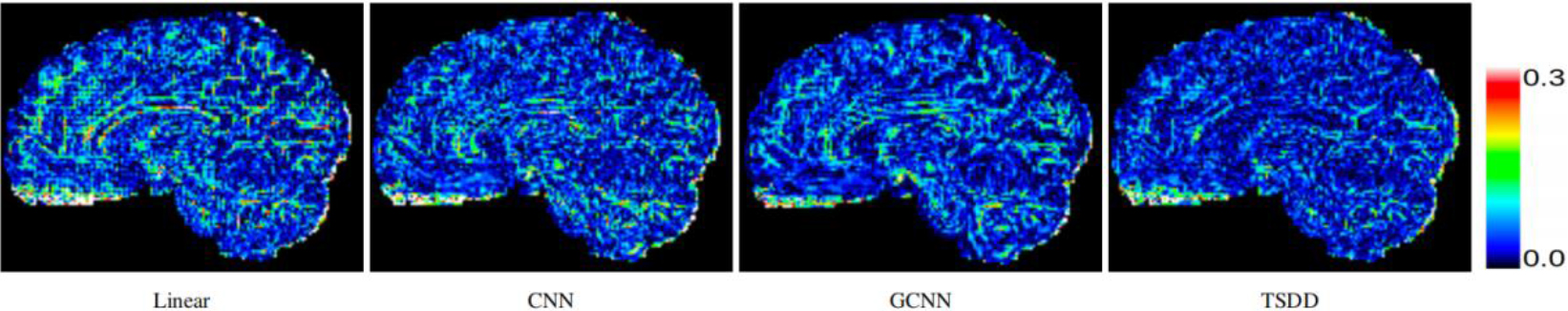
Comparison of error maps of the predicted HR DWI scans.

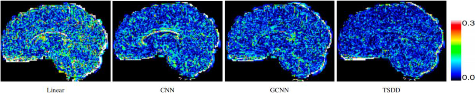
Figure 5.

Comparison of error maps of derived FA from reconstructed DWI scans.

3.4Results

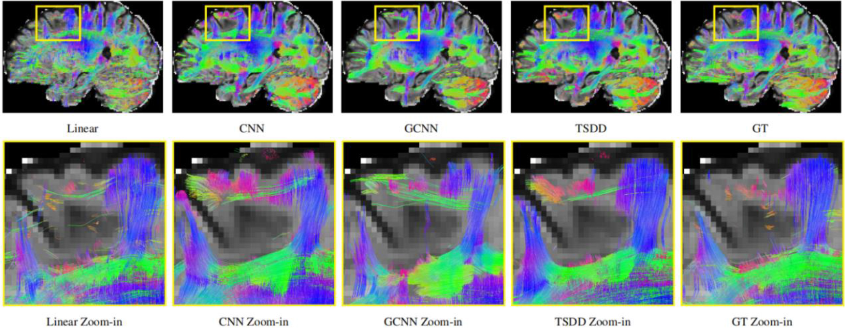
Comparisons were made on bicubic interpolation citation: CNN-only neural network and GCNN-only neural network with the same capacity of parameters. We also evaluated the quality of derived diffusion features, including fractional anisotropy (FA), fiber orientation distribution functions (fODFs) and fiber tracts. As shown in Fig. 3, the results of our proposed method were closer to the ground truth. We also computed the error maps for DWI and FA values (Figs 4 and 5). These figures show that our proposed method still achieved the best performance. The colored FA images are shown in Fig. 6. We zoomed in on some local regions of DWI scans, as shown in Fig. 7. These results indicated that our model achieved better performance with more structural details. fODFs are visualized in Fig. 8, indicating that the proposed model had coherent and clean fiber distributions close to the ground truth. We further performed tractography to evaluate our method. The fiber tracking results are visualized in Fig. 9, indicating that our model yielded rich fiber tracts extremely similar to the ground truth. All of the source images and their featured mappings were visualized using MRtrix3 [37].

Figure 6.

Comparison of the colored FA from the reconstructed HR DWI scans.

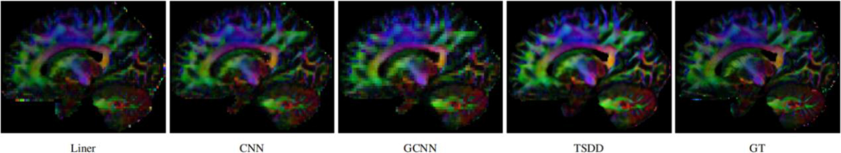
Table 1

Quantitative comparative analysis in terms of PSNR and SSIM

Model	Linear	NLM	CNN	GCNN	TSDD
DWI	29.69 and 0.90	30.16 and 0.92	30.49 and 0.95	28.29 and 0.94	33.52 and 0.96
FA	30.11 and 0.92	31.24 and 0.93	32.46 and 0.96	30.35 and 0.93	34.32 and 0.98

Figure 7.

Detailed comparison of the reconstructed DWI scans.

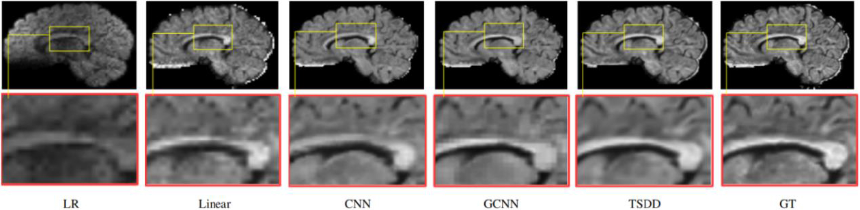
Figure 8.

Comparison of the fiber orientation distribution function (fODF).

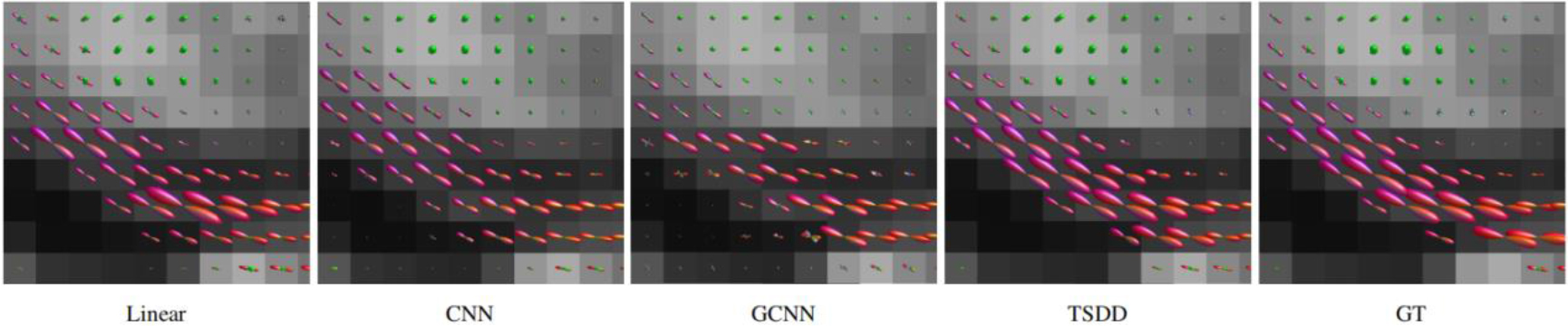
Figure 9.

Comparison of fiber tractography using different models.

The quantitative results are displayed in Table 1 As shown, the proposed method achieved the best performance in terms of PSNR and SSIM.

4.Discussion

In our experiments, the voxel value in DWI scans was normalized to [0–1], reducing the loss value. So, a smaller regulation coefficient was a reasonable choice in training, for example, 5 × 10^{- 6}. The nonzero rate was set to eliminate patches with too many zero voxels to crop the background and keep the boundary consistent. In our study, the value of the nonzero rate was set as 0.6. Additionally, the filter size in graph convolution is an extremely sensitive and time-consuming factor. Hence, a low-order polynomial can effectively contribute to stable learning on the graph. In our experiments, the best performance was achieved with a second-order Chebyshev polynomial.

5.Conclusions

In this study, we proposed a two-stage and domain-directed convolutional learning model for increasing the spatial resolution of LR DWI scans. In our proposed network, we used CNN and GCNN to extract spatial and angular information from grid structural and diffusion domains, respectively. Extensive experiments using HCP data demonstrated the improved performance of our proposed method in both qualitative and quantitative evaluations. Our model had the potential to be applied to other studies requiring learning from heterogeneous data domains.

Acknowledgments

The data for this study were partially sourced from the HCP, WU-Minn Consortium, led by principal investigators David Van Essen and Kamil Ugurbil (Grant No. 1U54MH091657). Funding for this project was provided by 16 NIH institutes and centers supporting the NIH Blueprint for Neuroscience Research, and by the McDonnell Center for Systems Neuroscience at Washington University. The data collection and sharing were facilitated by the MGH-USC HCP.

Conflict of interest

None to report.

References

[1]	Johansen-Berg H, Behrens TE. Diffusion MRI: from quantitative measurement to in vivo neuroanatomy: Academic Press; (2013) .
[2]	Coupe P, Manjon JV, Chamberland M, Descoteaux M, Hiba B. Collaborative patch-based super-resolution for diffusion-weighted images. NeuroImage. (2013) ; 83: : 245-261. doi: 10.1016/j.neuroimage.2013.06.030.
[3]	Chen G, Dong B, Zhang Y, Lin W, Shen, D, Yap, PT. XQ-SR: Joint x-q space super-resolution with application to infant diffusion MRI. Medical Image Analysis. (2019) ; 57: : 44-55. doi: 10.1016/j.media.2019.06.010.
[4]	Greenspan H, Oz G, Kiryati N, Peled S. MRI inter-slice reconstruction using super-resolution. (2002) ; 20: (5): 437-446. doi: 10.1016/S0730-725X(02)00511-8.
[5]	Pham CH, Ducournau A, Fablet R, Rousseau F. Brain mri super-resolution using deep 3d convolutional networks. In: Proceedings of the 2017 IEEE 14th International Symposium on Biomedical Imaging (ISBI 2017). IEEE; 2017. pp. 197-200. doi: 10.1109/ISBI.2017.7950500.
[6]	Dong C, Loy CC, He K, Tang X. Image super-resolution using deep convolutional networks. IEEE Transactions on Pattern Analysis and Machine Intelligence. (2016) ; 38: (2): 295-307. doi: 10.1109/TPAMI.2015.2439281.
[7]	Chen Y, Xie Y, Zhou Z, Shi F, Christodoulou AG, Li D. Brain mri super resolution using 3d deep densely connected neural networks. 2018 IEEE 15th international symposium on biomedical imaging (ISBI 2018). Washington D.C.; (2018) . pp. 739-742. doi: 10.1109/ISBI.2018.8363679.
[8]	Sanchez I, Vilaplana V. Brain mri super-resolution using 3d generative’ adversarial networks. (2018) ; arXiv preprint arXiv1812.11440.
[9]	Scherrer B, Gholipour A, Warfield SK. Super-resolution reconstruction to increase the spatial resolution of diffusion weighted images from orthogonal anisotropic acquisitions. Medical Image Analysis. (2012) ; 16: (7): 1465-1476. doi: 10.1016/j.media.2012.05.003.
[10]	Yin S, You X, Yang X, Peng Q, Zhu Z, Jing XY. A joint space-angle regularization approach for single 4d diffusion image super-resolution. Magnetic Resonance in Medicine. (2018) ; 80: (5): 2173-2187. doi: 10.1002/mrm.27184.
[11]	Alexander DC, Zikic D, Zhang J, Zhang H, Criminisi A. Image quality transfer via random forest regression: applications in diffusion mri. In: International Conference on Medical Image Computing and Computer Assisted Intervention. MA: Boston. (2014) ; pp. 225-232. doi: 10.1007/978-3-319-10443-0_29.
[12]	Xin Z, Lam EY, Wu EX, Wong KKY. Application of tikhonov regularization to super-resolution reconstruction of brain mri images. In: International Conference on Medical Imaging and Informatics. Beijing. (2007) ; pp. 46-51. doi: 10.1007/978-3-540-79490-5_8.
[13]	Manjon JV, Coupe P, Buades A, Fonov V, Collins DL, Robles M. Non-Local Mri Upsampling. (2010) ; 14: (6): 784-792. doi: 10.1016/j.media.2010.05.010.
[14]	Rueda A, Malpica N, Romero E. Single-image super-resolution of brain mr images using over-complete dictionaries. Medical Image Analysis. (2013) ; 17: (1): 113-132. doi: 10.1016/j.media.2012.09.003.
[15]	Tanno R, Worrall DE, Ghosh A, Kaden E, Sotiropoulos SN, Criminisi A, Alexander DC. Bayesian image quality transfer with cnns: Exploring uncertainty in dmri super-resolution. In: International Conference on Medical Image Computing and Computer-Assisted Intervention. QC: Quebec City. (2017) ; pp. 611-619. doi: 10.1007/978-3-319-66182-7_70.
[16]	Blumberg SB, Tanno R, Kokkinos I, Alexander DC. Deeper image quality transfer: training low-memory neural networks for 3d images. Springer. (2018) . doi: 10.1007/978-3-030-00928-1_14.
[17]	Fan M, Liu Z, Xu M, et al. Generative adversarial network-based super-resolution of diffusion weighted imaging: Application to tumour radiomics in breast cancer. NMR in Biomedicine. (2020) ; 33: (8): e4345. doi: 10.1002/nbm.4345.
[18]	Lim B, Son S, Kim H, Nah S, Lee K. Enhanced Deep Residual Networks for Single Image Super-Resolution. In: Proceedings of the IEEE International Conference on Computer Vision. NTIRE (New Trends in Image Restoration and Enhancement). IEEE Computer Society; (2017) . doi: 10.1109/CVPRW.2017.151.
[19]	Defferrard M, Bresson X, Vandergheynst P. Convolutional neural networks on graphs with fast localized spectral filtering, In: Advances in Neural Information Processing Systems. (2016) ; pp. 3844-3852. doi: 10.48550/arXiv.1606.09375.
[20]	Bruna J, Zaremba W, Szlam A, LeCun Y. Spectral networks and locally connected networks on graphs. arXiv preprint arXiv1312.6203. doi: 10.48550/arXiv.1312.6203.
[21]	Bronstein MM, Bruna J, LeCun Y, Szlam A, Vandergheynst P. Geometric deep learning: going beyond euclidean data. IEEE Signal Processing Magazine. (2017) ; 34: (4): 18-42. doi: 10.1109/MSP.2017.2693418.
[22]	Lee Y, Jeong J, Yun J, Cho W, Yoon KJ. Spherephd: Applying cnns on 360 images with non-euclidean spherical polyhedron representation. IEEE Transactions on Pattern Analysis and Machine Intelligence. (2020) ; 44: (2): 834-47. doi: 10.1109/TPAMI.2020.2997045.
[23]	Li G, Muller M, Thabet A, Ghanem B. Deepgcns: can gcns go as deep as cnns? In: Proceedings of the IEEE/CVF International Conference on Computer Vision (ICCV). (2019) . doi: 10.48550/arXiv.1904.03751.
[24]	Henaff M, Bruna J, LeCun Y. Deep convolutional networks on graphstructured data. arXiv arXiv preprint arXiv: 1506.05163. doi: 10.48550/arXiv.1506.05163.
[25]	Hammond DK, Vandergheynst P, Gribonval R. Wavelets on graphs via spectral graph theory. Applied and Computational Harmonic Analysis. (2009) ; 30: : 129-50. doi: 10.48550/arXiv.0912.3848.
[26]	Kipf TN, Welling M. Semi-supervised classification with graph convolutional networks. arXiv preprint arXiv: 1609.02907. doi: 10.48550/arXiv.1609.02907.
[27]	Ktena SI, Parisot S, Ferrante E, Rajchl M, Lee M, Glocker B, Rueckert D. Distance metric learning using graph convolutional networks: Application to functional brain networks, in: International Conference on Medical Image Computing and Computer-Assisted Intervention, Springer. (2017) ; pp. 469-477. doi: 10.1007/978-3-319-66182-7_54.
[28]	Huang G, Liu Z, Laurens VDM, Weinberger KQ. Densely connected convolutional networks. In: Proceedings of the IEEE Conference on Computer Vision and Pattern Recognition. (2017) ; pp. 4700-4708. doi: 10.1109/CVPR.2017.243.
[29]	Paoletti ME, Member S, IEEE Haut JM, Member S. Deep pyramidal residual networks for spectral–spatial hyperspectral image classification. IEEE Transactions on Geoscience and Remote Sensing. (2019) ; 57: (2): 740-754. doi: 10.1109/TGRS.2018.2860125.
[30]	Alom MZ, Yakopcic C, Nasrin MS, Taha TM, Asari VK. Breast cancer classification from histopathological images with inception recurrent residual convolutional neural network. Journal of Digital Imaging. (2019) ; 32: (4): 605-617. doi: 10.1007/s10278-019-00182-7.
[31]	Zhao X, Zhang Y, Zhang T, Zou X. Channel splitting network for single mr image super-resolution. IEEE Transactions on Image Processing. (2019) ; 28: (11): 5649-5662. doi: 10.1109/TIP.2019.2921882.
[32]	Essen DCV, Smith SM, Barch DM, Behrens TEJ, Ugurbil K. The wu-minn human connectome project: an overview. Neuroimage. (2013) ; 80: 62-79. doi: 10.1016/j.neuroimage.2013.05.041.
[33]	Andersson JL, Skare S, Ashburner J. How to correct susceptibility distortions in spin-echo echo-planar images: application to diffusion tensor imaging. Neuroimage. (2003) ; 20: (2): 870-888. doi: 10.1016/S1053-8119(03)00336-7.
[34]	Andersson JL, Sotiropoulos SN. Non-parametric representation and prediction of single-and multi-shell diffusion-weighted mri data using gaussian processes. Neuroimage. (2015) ; 122: : 166-176. doi: 10.1016/j.neuroimage.2015.07.067.
[35]	Andersson JL, Sotiropoulos SN. An integrated approach to correction for off-resonance effects and subject movement in diffusion mr imaging. Neuroimage. (2016) ; 125: : 1063-1078. doi: 10.1016/j.neuroimage.2015.10.019.
[36]	Wang Z, Bovik AC, Sheikh HR, Simoncelli EP. Image quality assessment: from error visibility to structural similarity. IEEE Transactions on Image Processing. (2004) ; 13: (4): 600-612. doi: 10.1109/tip.2003.819861.
[37]	Tournier JD, Smith R, Raffelt D, Tabbara R, Dhollander T, Pietsch M, et al. Mrtrix3: A fast, flexible and open software framework for medical image processing and visualisation. Neuroimage. (2019) ; 202: : 116-37. doi: 10.1016/j.neuroimage.2019.116137.