
Brain tumor segmentation based on the U-NET++ network with efficientnet encoder
Abstract
BACKGROUND:
Brain tumor is a highly destructive, aggressive, and fatal disease. The presence of brain tumors can disrupt the brain’s ability to control body movements, consciousness, sensations, thoughts, speech, and memory. Brain tumors are often accompanied by symptoms like epilepsy, headaches, and sensory loss, leading to varying degrees of cognitive impairment in affected patients.
OBJECTIVE:
The study goal is to develop an effective method to detect and segment brain tumor with high accurancy.
METHODS:
This paper proposes a novel U-Net
RESULTS:
The proposed segmentation model is trained and tested on Kaggle’s LGG brain tumor dataset, which obtains a satisfying performance with a Dice coefficient of 0.9180.
CONCLUSION:
This paper conducts research on brain tumor segmentation, using the U-Net
1.Introduction
Brain tumors are formed by the growth of abnormal cells in the brain. Accurate and reliable segmentation of brain tumors is crucial for diagnosis, treatment planning, and monitoring of tumor progression. However, due to the widespread use of MRI equipment in brain examination, a large amount of brain MRI images will be generated in the clinic, which is impossible for doctors to manually annotate and segment. Furthermore, due to the intricate neural structures within the brain, segmenting brain tumors can be particularly challenging. Patients may experience severe symptoms such as epilepsy, aphasia, dementia, and cognitive impairment after the surgery, resulting in irreversible damage. Cleanly segmenting tumor tissue and avoiding damage to normal nerve tissue can significantly drop the probability of the above-mentioned surgical sequelae and reduce tumor recurrence rate, which is crucial for mitigating the suffering of patients and prolonging the survival time.
Automatic segmentation networks have the ability to analyze a large amount of medical data to detect and segment tumors, usually getting segmentation results in a short time and achieving higher accuracy than manual diagnosis. This paper aims to separate tumor tissue and surrounding normal nerve tissue accurately with the help of deep learning algorithms. We propose a novel U-Net
2.Literature review
Some traditional machine learning algorithms such as support vector machine (SVM), conditional random field (CRF), and random forest (RF) are widely used in brain tumor segmentation tasks in the past few decades. Juan-Albarracín et al. [1] evaluated different unsupervised segmentation methods including K-means, Fuzzy K-means, GMM, GHMRF, which prove unsupervised segmentation algorithms are effective and competitive in brain tumor segmentation. Wu et al. [2] proposed a color-based K-means clustering segmentation method, which combines color transformation, K-means clustering and histogram clustering. This model provided good segmentation performance that helps doctors accurately detect the size and area of the tumor.
Later, with the innovation of hardware and other technologies, computing power is promoted. The development of deep learning is booming and shows vast advantages in the medical field. Mittal et al. [3] applied a model combining Stationary Wavelet Transform (SWT) and Growing Convolutional Neural Network (GCNN). SWT was used for feature extraction, and it has better results than Fourier transform on discontinuous data. After feature extraction, a random forest classifier was applied for segmentation and the GCNN network was used to train the model, which improved the brain tumor segmentation accuracy. Nema et al. [4] proposed a novel RescueNet network. The architecture consists of an encoding path (from 256
Researchers also found the encoder-decoder structure greatly improves the accuracy of image segmentation tasks. Ghosh et al. [5] used an improved U-Net framework to segment tumors, applying dense convolutional blocks during the downsampling process to enhance feature reusability. Meanwhile, VGG-16 architecture was used for the decoder. To improve model stability and performance, they added batchnormalization (BN) layers in the dense blocks. After performing a 5-fold cross-validation method on the TCGA-LGG dataset, this model got a Dice coefficient of 0.9099 and a Jaccard coefficient of 0.8189. The U-Net architecture has an encoder and decoder structure that preserves rich semantic features and provides excellent performance in image segmentation tasks.
Most current research efforts seek methods to obtain automated brain tumor segmentation results that provide objective, reproducible, and scalable methods for the quantitative assessment of brain tumors [6]. While the encoder-decoder architecture has been widely applied for brain tumor segmentation, choosing the optimal architecture remains a significant challenge. For example, many variants of U-Net exist, such as Residual U-Net [7], Dense U-Net [8], etc. Choosing an optimal U-Net architecture for more satisfactory performance and accuracy remains an important task.
3.Materials and methods
This paper proposes a U-Net
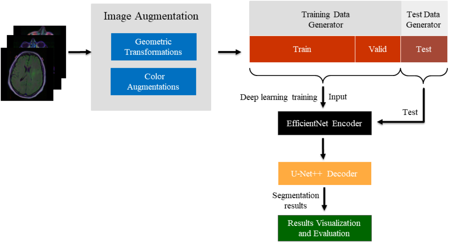
We apply image augmentation techniques, and the training data after augmentation is fed into the EfficientNet encoder for feature extraction, and then into the U-Net
Figure 1.
The flowchart of proposed segmentation model.
3.1Data collection
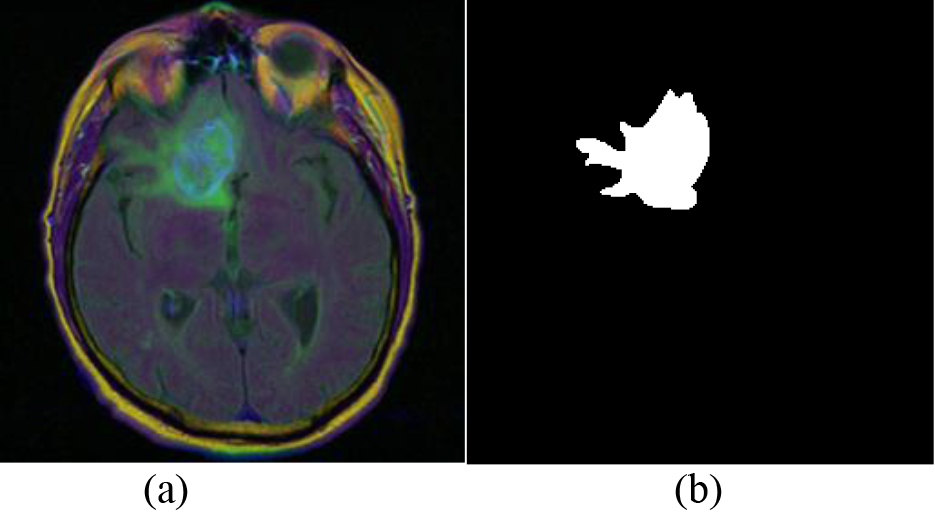
The dataset selected in this paper is the LGG Segmentation Dataset available on Kaggle, which is a reliable and widely used dataset in the brain tumor segmentation field. The dataset includes images from The Cancer Imaging Archive (TCIA) and data from 110 patients in the lower-grade glioma collection of The Cancer Genome Atlas (TCGA). Overall, the dataset contains 3929 sets of brain MRI images and corresponding manual segmentation masks. Specifically, it includes 2556 sets of normal morphological data without tumors and 1373 sets of abnormal MRI images with tumors. Figure 2 provides an illustrative example of the images present in the database, where (a) represents the brain MRI image and (b) depicts the corresponding manual segmentation mask.
Figure 2.
Details of dataset. (a) Brain MRI image. (b) Manual Segmentation mask.
3.2Image augmentations
Deep learning models rely heavily on a large amount of training data to achieve high accuracy. Insufficient data often cause overfitting problems and influences the performance of the model. However, in most computer vision tasks, the training data is very limited. Data augmentation techniques are helpful in this situation. Image augmentation makes a series of random changes like rotation, shifts, and flips to develop new training examples from the existing ones, efficiently reducing the model’s dependence on certain attributes.
In this research, we apply the Albumentations library for image augmentation. Albumentations [9] is a powerful data augmentation tool that contains lots of data augmentation methods such as image resizing, scale, rotation, transpose, flipping, etc. Meanwhile, the Albumentations package can simultaneously change the original images and corresponding mask images and provide high-speed processing speed, which is suitable and popular in segmentation tasks. In this paper, we set up the following augmentation methods using the Albumentations package:
(1) Set random HorizontalFlip by the ratio of 0.5;
(2) Set contrast limited adaptive histogram equalization (CLAHE) by a ratio of 0.5;
(3) Randomly select a transform in RandomGamma transform and RandomBrightness transform for the MRI images by the ratio of 0.3;
(4) Randomly select a transform in ElasticTransform and GridDistortion for the MRI images by the ratio of 0.3;
3.3EfficientNet encoder
EfficientNet [10] is a novel convolutional neural network architecture proposed by the Google team. It provides a family of models (EfficientNetB0 to EfficientNetB7) which can extract features efficiently and is considered the most state-of-the-art computer vision network nowadays. A convolutional neural network has three crucial dimensions: depth, width, and resolution. The depth of the network corresponds to the number of layers of the network, width corresponds to the number of neurons in the layer, and resolution is related to the height and width of the image. Usually, these three dimensions can be scaled to improve the learning effect of the model. Although choosing one among the three dimensions to scale can work out to improve the performance, when the dimension is scaled to a certain extent, the model’s accuracy will fall into a bottleneck and tend to be saturated. If we deepen the network depth, the model can learn more complex features but encounters the bottleneck of gradient disappearance. In this case, the network’s width and resolution should be changed to match the depth; Similarly, if the resolution is scaled, the network’s depth and width should also be increased to have a larger receptive field and capture more features. Through the cooperation of the three dimensions, the model can be scaled uniformly to achieve the best model effect and slow down the saturation speed of single-dimensional scaling. Compared with other models that only scale in one dimension, EfficientNet balances the three dimensions of depth, width, and resolution to avoid model saturation caused by scaling a single dimension.
To obtain the best combination of the three variables of width, depth, and resolution more efficiently, EfficientNet uses the following compound scaling method:
(1)
(2)
(3)
Where the value of
The EfficientNet family of models provides a set of scalable and efficient deep neural network architectures that can be customized to fit a wide range of computational and accuracy requirements. EfficientNet-B0 can be seen as the baseline network. EfficientNetB1-B7 are progressively larger and more complex. The best parameters of EfficientNet-B0 can be achieved by doing a small grid search over
At the same time, the EfficientNet model uses the Swish activation function. It is a product of linear and Sigmoid functions. The value of Swish activation function can be slightly negative around zero, resulting in a smoother gradient space and making the network easier to learn the data distribution. Compared with ReLU, the Swish activation function is more suitable for deeper networks. Equations (4) and (5) state the Swish activation function method:
(4)
(5)
In addition, EfficientNet can represent information with fewer channels. Hence, as the computational complexity of the decoder grows, EfficientNet can build a more computationally efficient system. When using a complex decoder like U-Net
3.4U-Net+ +
Traditional convolutional neural networks obtain deep features of the original images by reducing the resolution of images. However, such low-resolution feature maps usually lose useful spatial information that affects the segmentation accuracy. Models with an encoder-decoder structure, such as the U-Net network [12], are helpful in this condition. U-Net consists of a contracting path and an expanding path, which can restore spatial information and realize accurate segmentation. The network directly combines low-resolution but semantically-rich deep feature maps with high-resolution, fine-grained shallow feature maps by skip connections to recover details in target regions. However, directly combining the shallow feature map with the upsampling deep feature map obtained in the expansion path may have a large semantic gap, affecting the model’s effectiveness [13].
Compared with the U-Net network, U-Net
U-Net
(6)
Where
We extracted four feature maps of different sizes from the EfficientNet network as the input of the U-Net
Figure 3.
The structure of the proposed U-Net
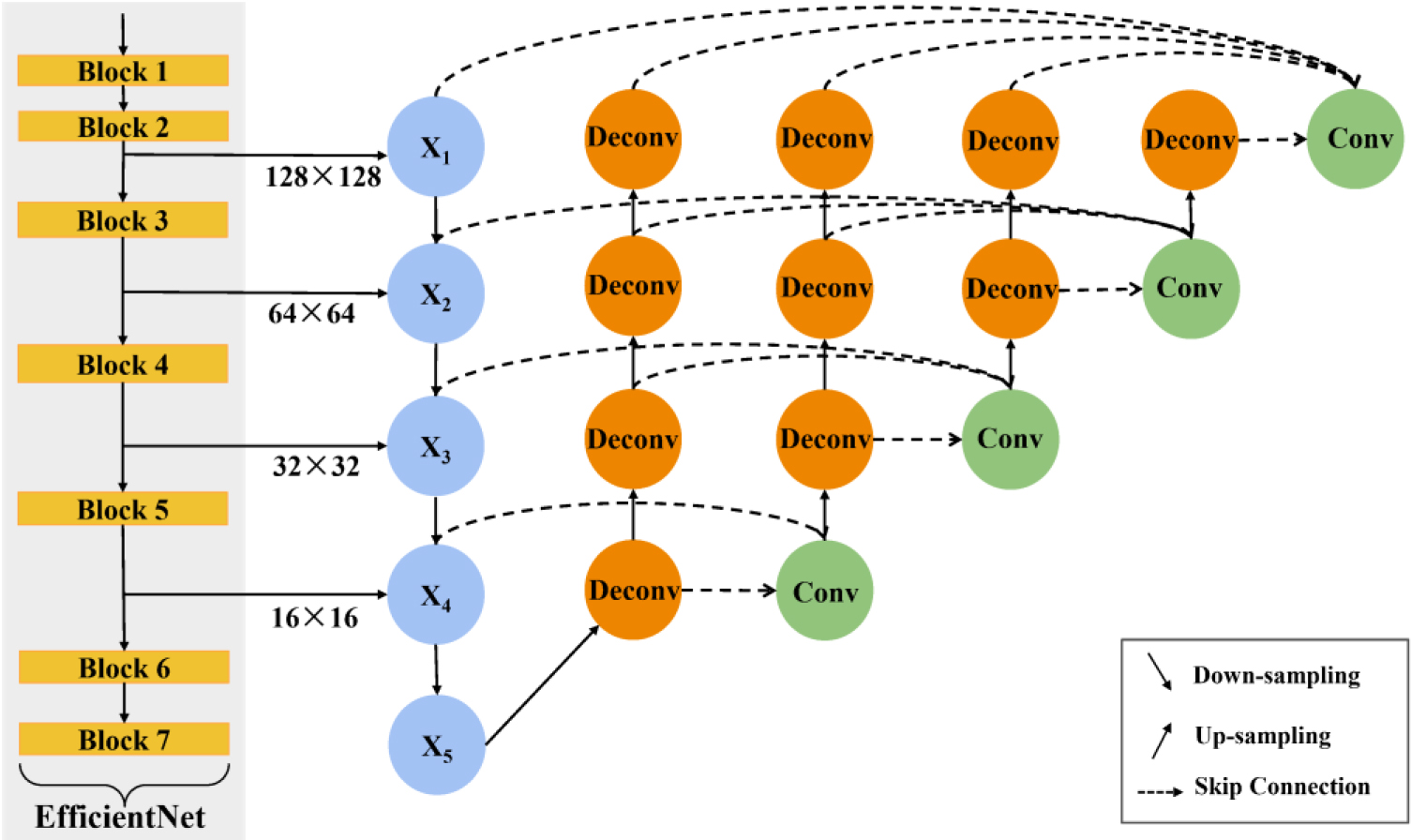
Compared with the original U-Net
3.5Loss function
Our segmentation model combines the cross-entropy loss function and the Dice loss function to take advantage of them. The model can be optimized under the control of both loss functions simultaneously. The calculation process of the cross-entropy loss function can be seen in Eq. (7).
(7)
In Eq. (7),
It predicts the category of each pixel and averages all the pixels. Therefore, when the pixel categories on the picture are unbalanced, mainstream pixels can easily dominate the training process, reducing the capability of extracting the weak pixel categories. The dice coefficient is a metric function used to measure the similarity of sets. It is usually used to calculate the pixel similarity between two samples, suitable for semantic segmentation tasks. The Dice loss function formula is shown below:
(8)
Where
In this paper, we combine the binary cross-entropy loss function and the dice loss function. The sum of the two loss functions is used as a measure of model loss. The Dice loss function calculates the proportion of overlap between the predicted segmentation results and the ground truth, which reduces the impact of imbalanced data on model optimization and alleviates the problem caused by the imbalance between foreground and background [15]. However, it may make the training process unstable. When the target area is small, the prediction error of some pixels will cause a huge fluctuation in the loss value. Both the cross-entropy loss function and the Dice loss function have their shortcomings, so we combine the cross-entropy with the Dice loss function to help improve the stability of the model.
4.Results and discussion
In our experiment, the Adam optimizer was selected, which is a stochastic gradient-based optimization. The Adam optimizer is computationally efficient, requires little memory, and only requires first-order gradients [16]. Besides, ImageNet pre-trained weights are used to initialize the EfficientNet model, which provides a reasonable initial weight of the encoder and avoids overfitting problems. We divide the dataset into training set, validation set, and test set at a ratio of 8:1:1. There are 100 epochs in the training process, and the learning rate is dynamically adjusted during the process with an initial learning rate of 0.001. We utilize the cosine annealing [17] to adjust the learning rate, which can prevent the training from falling into a local optimal value.
We adopt the Dice coefficient to evaluate the segmentation results in this experiment, which can calculate the similarity of two samples and is effective in segmentation tasks. Equation (9) shows the computing process of Dice coefficient. To ensure the reliability of the results, we experiment 10 times and take the average value as the final result.
(9)
In Eq. (9),
In our experiment, the EfficientNetB4 encoder is applied. The encoder is initialized by ImageNet weight to avoid model overfitting. The encoder output layers with shapes of 16
Table 1
Results of different EfficientNet encoder
| Model | Dice coefficient |
|---|---|
| EfficientNetB0 | 0.9177 |
| EfficientNetB4 | 0.9180 |
Figure 4.
Segmentation model results.
To compare the effect of different EfficientNet encoders, we apply EfficientNetB0 and EfficientNetB4 from the EfficientNet family as the encoder, respectively. Both EfficientNetB0 and EfficientNetB4 are initialized with ImageNet pre-trained weights. The Dice coefficient results are demonstrated in Table 1.
Table 1 shows the segmentation model with EfficientNetB0 as the encoder obtains a Dice coefficient of 0.9177. The EfficientNetB4 encoder has more channels and model parameters, and therefore has the ability to learn more feature information, performing slightly better than EfficientNetB0.
Additionally, to compare the impact of the loss function on the proposed segmentation model, we conduct experiments using four different loss functions. All the loss functions are experimented with the EfficientNetB4 encoder to control variables. We compare the Dice loss function, cross-entropy loss function, Focal loss function [18], and loss function combining cross-entropy and Dice loss. The focal loss function is an extension of the cross-entropy loss function. Equation (10) shows the calculation process of it. Compared with the Dice loss function, the Focal loss function focuses on balancing hard and easy samples. It allows the model to focus on hard, misclassified examples by assigning weights, avoiding easy-to-classify data dominating the overall loss value.
(10)
Where
Table 2
Results of different loss functions
| Loss function | Dice coefficient |
|---|---|
| Dice Loss | 0.9163 |
| Cross-entropy Loss | 0.9130 |
| Focal Loss | 0.9088 |
| Cross-entropy | 0.9180 |
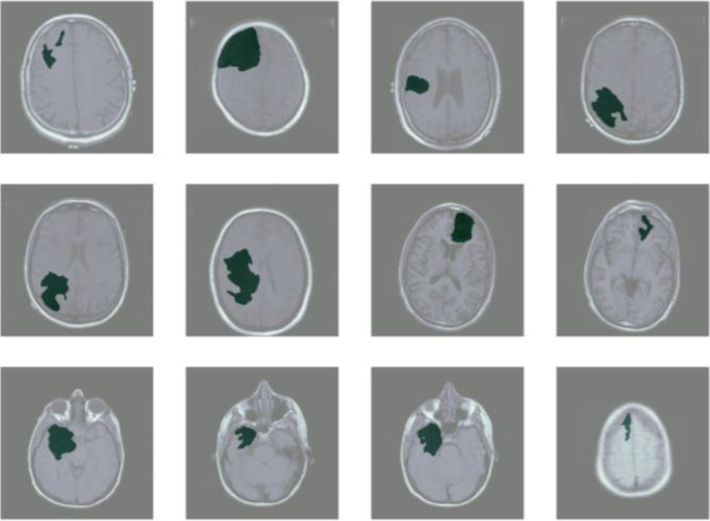
Figure 5.
Ground truth brain tumor mask.
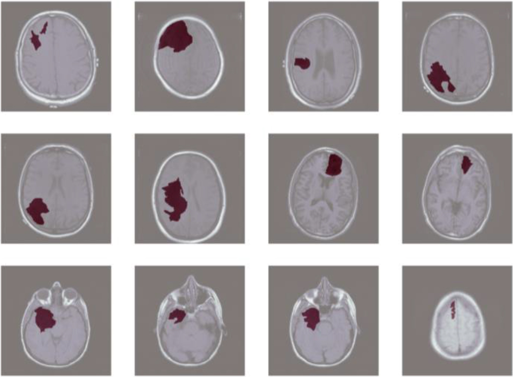
Table 2 details specific experimental results of different loss functions. Results in Table 2 show that the loss function combining the cross-entropy and Dice loss has the best performance. The model’s optimization effect using the cross-entropy loss function or the Dice loss function alone is not as good as the combined effect of the two on the model. The focal loss function is expected to have good performance since it extends the cross-entropy loss function and avoids the domination of easy-to-classify samples. However, results show that the Focal loss function performs the worst on this dataset among the four loss functions. The reason may be attributed to the large number of learnable samples we have provided through data augmentation technology. This approach increased the diversity of the dataset and provided the model with more examples to learn from. As a result, the advantage of the Focal loss function in addressing class imbalance was diminished.
In addition, to verify the effectiveness of the network, this paper compares the performance of this U-Net
Table 3
Comparison of other segmentation models
| Authors | Models | Dice coefficient |
|---|---|---|
| Tamer A19 | U-Net | 89.02% |
| Sourodip Ghosh5 | U-Net | 90.99% |
| Liping Yi20 | SU-Net | 78.5% |
| Rai H M21 | Vanilla U-Net | 82.06% |
|
| Proposed model | 91.80% |
5.Conclusions
Precise segmentation of brain tumors provides important support for neuropathological analysis, diagnostic report generation, surgical plan design, and treatment plan formulation. The complex anatomy of brain tumors makes manually segmentation time-consuming and easily affected by subjective factors. Therefore, establishing efficient algorithms to segment brain tumors automatically have great clinical significance.
In recent years, the development of medical imaging technology and deep learning algorithms has promoted the progress of related work. This paper conducts research on brain tumor segmentation, using the U-Net
The proposed U-Net
Acknowledgments
This study was supported by the (1) Key Open Project of Key Laboratory of Data Science and Intelligence Education (Hainan Normal University), Ministry of Education (DSIE202303); (2) Open Fund of Key Laboratory of Embedded System and Service Computing (Tongji University) under Grant ESSCKF 2022–03; (3) the National Natural Science Foundation of PR China (No. 12261029); and (4) the Higher Education Project of Hainan Provincial Department of Education (No. HnjgY2022ZD-4).
Conflict of interest
None to report.
References
[1] | Juan-Albarracín J, Fuster-Garcia E, Manjon JV, et al. Automated glioblastoma segmentation based on a multiparametric structured unsupervised classification. PloS One. (2015) ; 10: (5): e0125143. |
[2] | Wu MN, Lin CC, Chang CC. Brain tumor detection using color-based k-means clustering segmentation. Third International Conference on Intelligent Information Hiding and Multimedia Signal Processing (IIH-MSP 2007). IEEE. Vol. 2. (2007) . pp. 245-250. |
[3] | Mittal M, Goyal LM, Kaur S, et al. Deep learning based enhanced tumor segmentation approach for MR brain images. Applied Soft Computing. (2019) ; 78: : 346-354. |
[4] | Nema S, Dudhane A, Murala S, et al. RescueNet: An unpaired GAN for brain tumor segmentation. Biomedical Signal Processing and Control. (2020) ; 55: : 101641. |
[5] | Ghosh S, Chaki A, Santosh KC. Improved U-Net architecture with VGG-16 for brain tumor segmentation. Physical and Engineering Sciences in Medicine. (2021) ; 44: (3): 703-712. |
[6] | Magadza T, Viriri S. Deep learning for brain tumor segmentation: A survey of state-of-the-art. Journal of Imaging. (2021) ; 7: (2): 19. |
[7] | He K, Zhang X, Ren S, et al. Deep residual learning for image recognition. Proceedings of the IEEE Conference on Computer Vision and Pattern Recognition. (2016) . pp. 770-778. |
[8] | Huang G, Liu Z, Van Der Maaten L, et al. Densely connected convolutional networks. Proceedings of the IEEE Conference on Computer Vision and Pattern Recognition. (2017) . pp. 4700-4708. |
[9] | Buslaev A, Iglovikov VI, Khvedchenya E, et al. Albumentations: fast and flexible image augmentations. Information. (2020) ; 11: (2): 125. |
[10] | Tan M, Le Q. Efficientnet: Rethinking model scaling for convolutional neural networks. International Conference on Machine Learning. PMLR. (2019) . pp. 6105-6114. |
[11] | Silva JL, Menezes MN, Rodrigues T, et al. Encoder-decoder architectures for clinically relevant coronary artery segmentation. arXiv preprint arXiv2106.11447. (2021) . |
[12] | Ronneberger O, Fischer P, Brox T. U-net: Convolutional networks for biomedical image segmentation. International Conference on Medical Image Computing and Computer-Assisted Intervention. Springer, Cham. (2015) . pp. 234-241. |
[13] | Le Duy Huynh NB. A U-NET++ with pre-trained EfficientNet backbone for segmentation of diseases and artifacts in endoscopy images and videos. CEUR Workshop Proceedings. (2020) ; 2595: : 13-17. |
[14] | Zhou Z, Rahman Siddiquee MM, Tajbakhsh N, et al. Unet |
[15] | Zhao R, Qian B, Zhang X, et al. Rethinking dice loss for medical image segmentation. 2020 IEEE International Conference on Data Mining (ICDM). IEEE. (2020) . pp. 851-860. |
[16] | Zhang D, Chen Y, Chen Y, et al. Heart disease prediction based on the embedded feature selection method and deep neural network. Journal of Healthcare Engineering. (2021) . 2021. |
[17] | Loshchilov I, Hutter F. Sgdr: Stochastic gradient descent with warm restarts. arXiv preprint arXiv1608.03983. (2016) . |
[18] | Lin TY, Goyal P, Girshick R, et al. Focal loss for dense object detection. Proceedings of the IEEE International Conference on Computer Vision. (2017) . pp. 2980-2988. |
[19] | Tamer A, Youssef A, Ibrahim M, et al. Deep learning techniques for the fully automated detection and segmentation of brain MRI. 2022 5th International Conference on Computing and Informatics (ICCI). IEEE. (2022) . pp. 310-315. |
[20] | Yi L, Zhang J, Zhang R, et al. SU-net: an efficient encoder-decoder model of federated learning for brain tumor segmentation. International Conference on Artificial Neural Networks. Springer, Cham. (2020) . pp. 761-773. |
[21] | Rai HM, Chatterjee K, Dashkevich S. Automatic and accurate abnormality detection from brain MR images using a novel hybrid UnetResNext-50 deep CNN model. Biomedical Signal Processing and Control. (2021) ; 66: : 102477. |


