Location verification algorithm of wearable sensors for wireless body area networks

Wang, Hua; Wen, Yingyou; Zhao, Dazhe

doi:10.3233/THC-173812

Location verification algorithm of wearable sensors for wireless body area networks

Issue title: Papers from the 6th International Conference on Biomedical Engineering and Biotechnology (iCBEB2017), 17–20 October 2017, Guangzhou, China

Guest editors: Carlos Gómez, Severin P. Schwarzacher and Huiyu Zhou

Article type: Research Article

Authors: Wang, Hua^{a; b; c; d} | Wen, Yingyou^{a; b; c; d} | Zhao, Dazhe^{a; e; *}

Affiliations: [a] School of Computer Science and Engineering, Northeastern University, Shenyang 110819, Liaoning, China | [b] State Key Laboratory of Software Architecture, Neusoft Corporation, Shenyang 110179, Liaoning, China | [c] Research Center of Safety Engineering Technology in Industrial Control, Neusoft Group Research, Shenyang 110179, Liaoning, China | [d] Engineering Research Center of the Ministry of Education in Security Protection for Complex Networks and Systems, Northeastern University, Shenyang 110819, Liaoning, China | [e] Key Laboratory of Medical Image Computing, Ministry of Education, Northeastern University, Shenyang 110819, Liaoning, China

Correspondence: [*] Corresponding author: Dazhe Zhao, Key Laboratory of Medical Image Computing, Ministry of Education, Northeastern University, Shenyang 110819, Liaoning, China. Tel.: +86 13804016931; E-mail: [email protected].

Keywords: Barometric altimetry, health monitoring system, location verification, medical monitoring, received signal strength indication, wearable wireless sensors, wireless body area network

DOI: 10.3233/THC-173812

Journal: Technology and Health Care, vol. 26, no. S1, pp. 3-18, 2018

Published: 29 May 2018

Get PDF

Abstract

BACKGROUND:

Knowledge of the location of sensor devices is crucial for many medical applications of wireless body area networks, as wearable sensors are designed to monitor vital signs of a patient while the wearer still has the freedom of movement. However, clinicians or patients can misplace the wearable sensors, thereby causing a mismatch between their physical locations and their correct target positions. An error of more than a few centimeters raises the risk of mistreating patients.

OBJECTIVE:

The present study aims to develop a scheme to calculate and detect the position of wearable sensors without beacon nodes.

METHODS:

A new scheme was proposed to verify the location of wearable sensors mounted on the patient’s body by inferring differences in atmospheric air pressure and received signal strength indication measurements from wearable sensors. Extensive two-sample t tests were performed to validate the proposed scheme.

RESULTS:

The proposed scheme could easily recognize a 30-cm horizontal body range and a 65-cm vertical body range to correctly perform sensor localization and limb identification.

CONCLUSIONS:

All experiments indicate that the scheme is suitable for identifying wearable sensor positions in an indoor environment.

1.Introduction

Wireless body area networks (WBANs) are also called body sensor networks and can also be used widely in military, sports, medicine, and other fields. In military, especially along borders where terrorists attack at any time, WBANs are a good fit. In sports, the physical fitness of an athlete can be checked using the WBAN technology. In medicine, WBANs have emerged as a vital technology capable of providing better methods to diagnose various hazardous diseases [1]. This technology can be used for patients suffering from asthma, heart problem, diabetes, Alzheimer’s disease, Parkinson’s disease, and others. Handicapped people can benefit from this technology if they are blind, as retina prosthesis chips can be implanted within the human eye to improve the vision quality [2]. Nano and microdevices are developed and implanted in, on, or around the human body to measure different physiological signals. Different heterogeneous sensors, for example electrocardiogram sensors, electroencephalogram sensors, and blood pressure measuring sensors, could be used to monitor different body parameters.

Figure 1.

An example of WBAN platform illustrating possible on-body sensor types and its environment [3].

Figure 2.

Two algorithms of the proposed scheme.

WBANs typically consist of a group of collaborating wearable sensors placed on near or within several locations of the human body, individually or through a combination (Fig. 1) [3, 4].

Wearable sensors are vital in on-body medical applications. They can be worn attached to the body in the form of adhesive pads, armbands, and leg straps, and removed for daily activities such as bathing or swimming, where sensors may get damaged. However, this flexibility enhances the opportunity of misplacement of sensors. For instance, a clinician, who detected dyskinesia symptoms in a patient with Parkinson’s disease, might obtain conflicting information if the physical placement of a sensor mismatches with its true target position. This mismatch might arise from wrong placement by patients or skilled medicine personnel. However, research on detecting node placement is still limited.

Motivated by the aforementioned observation, this study focuses on designing a new scheme to calculate and detect the positions of wearable sensors without beacon nodes know their own locations. Wearable sensors worn around the body can consist of identical hardware to minimize the design and manufacturing cost. Once the location of the wearable sensor is known, the examination can be carried out by using the corresponding programs. Each diagnosis need not be designed and programmed differently. As illustrated in Fig. 2, the proposed scheme is composed of two algorithms: Barometric altimetry verification (BAV) and received signal strength indication (RSSI)-based left or right identification (RBLRI). In BAV, the instantaneous air pressure at the location of each wearable sensor is measured and analyzed to calculate the vertical location of the sensor on a scale relative to the wearer. RBLRI demonstrates that each wearable sensor is capable of detecting distance changes sufficient to distinguish between the relative location of the patient’s left and right limb, thus making it possible to recognize which wearable sensor is placed on which limb.

The air pressure remains relatively stable in the horizontal direction with distance, but is quite sensitive to changes in the vertical direction. BAVBAV uses instantaneous air pressures to eliminate measurement errors arising from the irregular changes of atmospheric pressure. However, RSSI is dependent on the environment. In indoor environments, the wireless channel is quite noisy, and the radio frequency signal can suffer from reflection, diffraction, and multipath effect [5]. These factors can make the RSSI values fluctuate. To address the problem, the present study performs the RSSI treatment processing under a clear line of sight to determine the best area for the location verification of wearable sensors. RSSI is measured in the selected optimal areas by analyzing and optimizing the measurements. Such a scheme would, once per sensor placement, automatically calculate the sensor locations and provide immediate self-compensates.

The proposed scheme contains the following general features:

(1) It determines the vertical arrangement of wearable sensors mounted along the height of a patient’s body using the barometric height formula and measuring instantaneous air pressures at sensors.
(2) It distinguishes the horizontal location of wearable sensors by employing the ranging model and measuring RSSI values at sensors. Considering the effect of the working environment on the relationship between RSSI and distance, it determines the patient’s standing position to improve RSSI measurement accuracy.
(3) It performs two-sample t tests to experimentally infer the differences in pressures and RSSI values from wearable sensors.

The organization of the rest of the study is as follows. Section 2 describes related studies about limb position recognition. Section 3 describes the system structure. Section 4 introduces the barometric height formula and experimentally verifies the BAV approach. Section 5 introduces the RSSI ranging model and the effect of the working environment on signal strength measurements, and experimentally verifies the proposed RBLRI method. Section 6 provides the conclusion.

2.Related work

Previous studies referenced in this field focus on WBANs measurements based on costly pieces of equipment, either for channel-modeling purposes [6] or for the validation of on-body localization algorithms based on impulse radio [7, 8, 9, 10]. A previous study presents a technique to capture motion data to estimate the positions of sensors on the user’s body, employing mixed supervised and unsupervised learning approaches [11]. It can achieve 89% accuracy in determining the location of the device. However, this technique needs off-body processing and 30-min motion information, which makes it unsuitable for real-time limb monitoring. Moreover, the obtained accuracy greatly depends on the measured limb. Another study proposes an automatic identification method (AIM) enabling unassisted sensor nodes to continuously monitor node locations [12]. However, the scheme merely addresses the verification problem of the vertical location of the sensor, which limits the scope of application of the scheme.

RSSI has the advantages of low cost, low power, and accessibility; therefore, it becomes the most used technology in a diverse range of systems [13]. Even for noisy indoor environments, an average positioning error of 50 cm on an area of 3.5 × 4.5 m2 is possible by choosing the radio frequency and algorithm parameters carefully based on empirical studies [14]. However, introducing the RSSI localization technology into the localization of sensors for WBANs remains unexplored.

Motivated by the aforementioned observation, the present study used air pressures and RSSI measurements to determine the positions of wearable sensors, without the help of stationary hardware. The present study is novel in combining the barometric altimetry technology with RSSI localization technology to present a verification scheme that can distinguish which wearable sensor is placed on which limb (especially, identifying the left or right limb).

The proposed scheme contains the following obvious advantages:

(1) It is capable of monitoring distance changes to recognize which wearable sensor is placed on which limb. By this scheme, individual elements of the sensor can be easily replaced or compensated for to allow further operation.
(2) It can distinguish between different wearable sensors attached at the same altitude on the patient’s body.
(3) It can improve the security of wearable sensors for medical applications, as it guarantees the correct localization of each node mounted on the patient’s body.
(4) It depends neither on considerable sensors to execute localization nor on beacons that know their own locations to execute distance measurement.
(5) It can be easily extended to more than four wearable sensors for medical applications.

Figure 3.

Topology of WBAN platform.

3.System architecture

The prototype system consists of four wearable sensors, two RSSI transmitters, a base station (BS), and a personal computer (PC), as illustrated in Fig. 3. The Crossbow TelosB sensor node is employed in this study because of its ready-to-use format. Moreover, each wearable sensor on the patient’s limb has an added high-precision and low-power air pressure sensor, Bosch BMP180. RSSI transmitters periodically send singles to wearable sensor nodes. One RSSI transmitter is placed on the floor and the other at the height 0.8 m above the floor. Wearable sensors transmit the measured data to BS, which in turn forwards this data to the PC connected to it.

Figure 4.

Trend of altitude with air pressure.

Figure 5.

The barometric altimetry verification method.

4.Barometric altimetry verification

In this section, we develop a barometric altimetry verification to verify the vertical location of the sensor placed on the body.

Table 1

BAV algorithm

Algorithm 1. barometric altimetry verification
1. Initialize.
2. Read the received pressures from wearable sensors placed at the reference height.
3. Calculate the offset of each sensor and calibrate to the reference pressure data.
4. Read the received pressures from wearable sensors placed on the patient’s limb.
5. Calculate the pressure data by using the stored offset of each sensor.
6. Calculate the vertical arrangement of sensors by performing the two-sample t tests.

4.1Barometric height formula

Barometric altimetry is a traditional method to measure the altitude [15]. According to the theory of atmosphere physics [16], the vertical movement of the atmosphere is small and can be estimated in a static equilibrium state. Therefore, force in the horizontal direction cancels the net upward pressure in the vertical direction and reaches equilibrium with its own gravity. According to the standard atmospheric regulations [16], the air temperature varies linearly with height in a polytropic atmosphere. The height can be calculated as a function of the pressure under standard atmospheric conditions:

(1)

h=44331⁢[1-(P1013.25)0.19],

where P0 is the atmospheric pressure at sea level with a value 1013.25 hPa. The relationship between air pressure and altitude is illustrated in Fig. 4. The BAV is based on the theory that pressures decrease exponentially with increasing altitude.

To minimize the pressure variations resulting from various factors, such as time and weather, the instantaneous pressures are measured to identify the vertical locations of the sensors on a scale relative to the patient, as described in Fig. 5.

4.2Calibration

Generally, a principle of “uncertainty” is reflected in the measurement of air pressure. During the initial stages of the experiments, the sensors placed near one another yielded different air pressure values at the same altitude. The sensors still yielded different values after being moved the same distance vertically. This indicated that the differences in pressure readings resulting from factory calibration coefficients differ for each sensor. The differences do not change over time. Therefore, a constant offset calibration procedure is significant to enable a reliable barometric-based WBAN location verification.

The proposed scheme is calibrated by obtaining a number of samples at a reference position (altitude h= 0 m). The offset of each sensor is determined using differences between its own and the average pressure. This offset is stored for further elevation measurement. Because the deviation in sensors is considered to be nonlinear, the calibration process is repeated at different pressure measurement experiments to improve the accuracy of pressure data. The BAV algorithm is described in Table 1.

4.3Air pressure measurement and results

The proposed method mainly utilizes differences among air pressures worn on the patient’s limbs, to obtain the precise altitudes of wearable sensors, with the help of calibration process. The detailed measurement process is as follows:

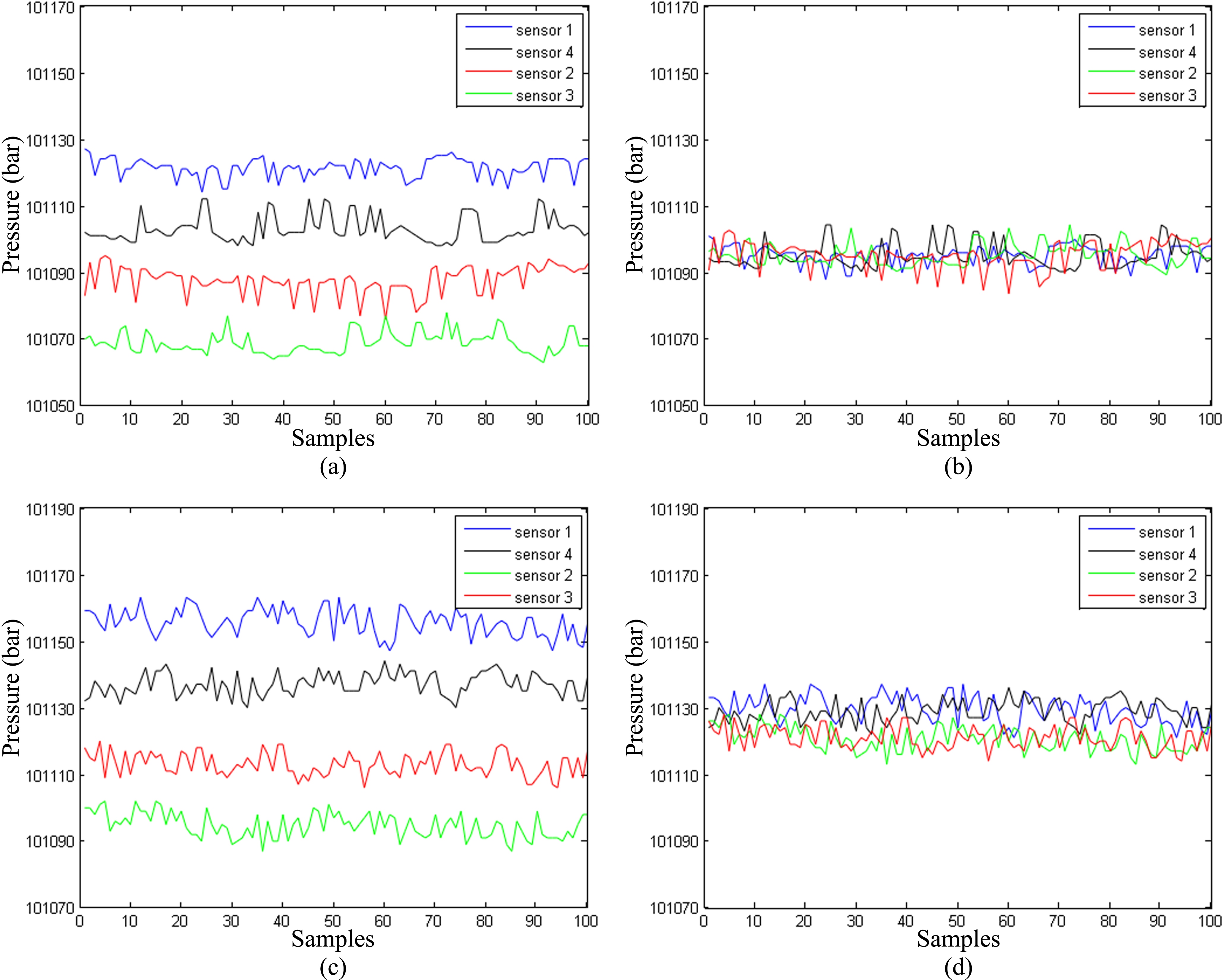
(1) Calibration: Sensor nodes are placed on the same reference position (i.e., floor) to ensure consistency. Software requests 100 samples of atmospheric pressure data from each device. Figure 6a displays the measurement results at the same reference position and the deviation errors among sensors. In Fig. 6b, the offset of each sensor is calculated, and the deviation correction of sensors 1, 2, 3 and sensor 4 measurement data is performed.
(2) Measurement: The sensor nodes are placed on the patient’s limbs, and 100 measurement data are collected from each wearable sensor in this step. Pressure readings at each wearable sensor are taken simultaneously. Figure 6c illustrates the pressure measurements obtained from air pressure sensors. Deviation corrections of all pressure data, taking into account the calibration performed, are illustrated in Fig. 6d.

Table 2

Comparison of means and standard deviations for the two methods

Sensor	BAV		AIM
	M (Pa)	SD	M (Pa)	SD
Sensor 1	101129.61	4.08	101131.11	4.67
Sensor 2	101120.72	3.75	101121.99	4.26
Sensor 3	101121.09	3.52	101118.00	5.95
Sensor 4	101129.02	3.42	101129.18	3.74

Figure 6.

(a) Air pressure measurements at the same reference position. (b) Deviation correction to the measurements. (c) Air pressure measurements for the patient’s limb. (d) Deviation correction to the measurements.

The proposed method was compared with the automatic identification method (AIM) [12] to evaluate the effectiveness of BAV. First, the performance of two methods in terms of the mean (M) and standard deviation (SD) are investigated. Table 2 indicates that the performance of the proposed method is obviously better than those in previous studies. AIM has a large fluctuation in the pressure measurement. BAV achieves an SD of 3.42–4.078, while it is 3.74–5.95 for AIM.

The significant difference of the present approach is compared with AIM through two-sample t tests to accurately identify the locations of nodes.

Table 3

Comparison of significant differences for the two methods

Group	Sensor	BAV			AIM
		Δ⁢P	Δ⁢P (95%CI)	P	Δ⁢P	Δ⁢P (95%CI)	P
		(Pa)	(Pa), (Pa)		(Pa)	(Pa), (Pa)
1	Sensor 1	8.90	7.80, 9.98	0.00	9.12	7.87, 10.37	0.00
	Sensor 2
2	Sensor 1	8.52	7.46, 9.58	0.00	13.12	11.63, 14.61	0.00
	Sensor 3
3	Sensor 1	0.59	-0.46, 1.64	0.27	0.93	0.55, 2.11	0.17
	Sensor 4
4	Sensor 2	-0.37	-1.39, 0.65	0.47	2.16	1.56, 3.44	0.09
	Sensor 3
5	Sensor 2	8.30	7.30, 9.30	0.00	-7.19	-8.31, -6.07	0.00
	Sensor 4
6	Sensor 3	7.93	6.96, 8.90	0.00	-11.19	-12.58, -9.8	0.00
	Sensor 4

Table 3 reveals that except for groups 3 and 4, all P values are below 0.05 for the two methods. This indicates that pressure differences between sensors are statistically different enough to distinguish heights of sensors, confirming that the two positions are indeed different with > 99.9% confidence interval (CI). Except for groups 3 and 4, BAV has an estimated difference of 6–9 Pa with a 95% CI, while it is 6–14 Pa for AIM. This is mainly because BMP085 can detect air pressure differences of 3 Pa, which for the BMP180 is 2 Pa. So 2 Pa. Therefore, AIM has a larger difference range.

In groups 3 and 4, the P values > 0.05 indicate that the data cannot be used to statistically reject sensors 1 and 4 at different heights, and thus, sensors 1 and 4 may be the leg nodes or the wrist nodes at the same time, so do sensors 2 and 3. Besides, the lower the air pressure, the higher the altitude. Consequently, both sensors 1 and 4 are the leg nodes, as well as both sensors 2 and 3 are the wrist nodes. Moreover, two P values of BAV are bigger than those of AIM. This also indicates that the average height difference of BAV is smaller than that of AIM. Therefore, the proposed BAV outperforms AIM in terms of pressure accuracy.

Therefore, BAV can achieve a much better performance on the vertical arrangement verification with very delectable results.

5.RSSI-based left or right identification

The proposed RBLRI is based on the distance estimation between the RSSI transmitter and the wearable sensor to recognize whether the sensor is placed on the left limb or the right limb.

5.1Ranging model

The power of a signal traveling between sensors is the signal parameters, which include the information that reflects the distance [17]. At present, wireless signal transmission uses the theoretical shadowing model widely [18]. The theoretical model is shown in [19]:

(2)

P=P0-10⁢n⁢lg⁡(dd0)+Xσ

where d0 is the reference distance, P0 is the radio power at the distance d0, and n is the path loss coefficient related to the environment Generally n= 2–6 [20]. Xσ∼(μ2) is a Gaussian distributed random variable. Let d0= 1 m, and ignore Xσ in the actual localization measurement Therefore, the shadowing transmission model can be written as:

(3)

𝑅𝑆𝑆𝐼=-(A+10⁢n⁢lg⁡d)

where RSSI is the received signal strength indication at a distance d from the transmitter and A is an empirical parameter, which is determined by measuring the RSSI value of 1 m from the transmitter [21]. The attenuation is somehow coherent with the general philosophy of the log-normal shadowing the propagation model. RSSI decreases as a function of the log of the distance [22]. Hence, the identification problem can be simplified to evaluate the RSSI values from the wearable sensors.

Figure 7.

An RSSI value between sensors under different heights.

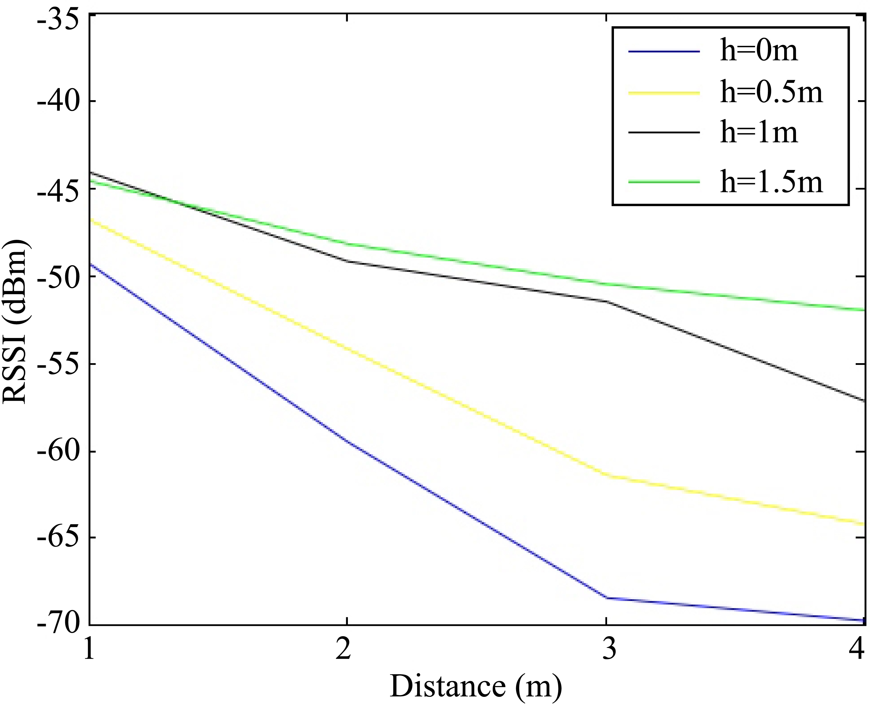
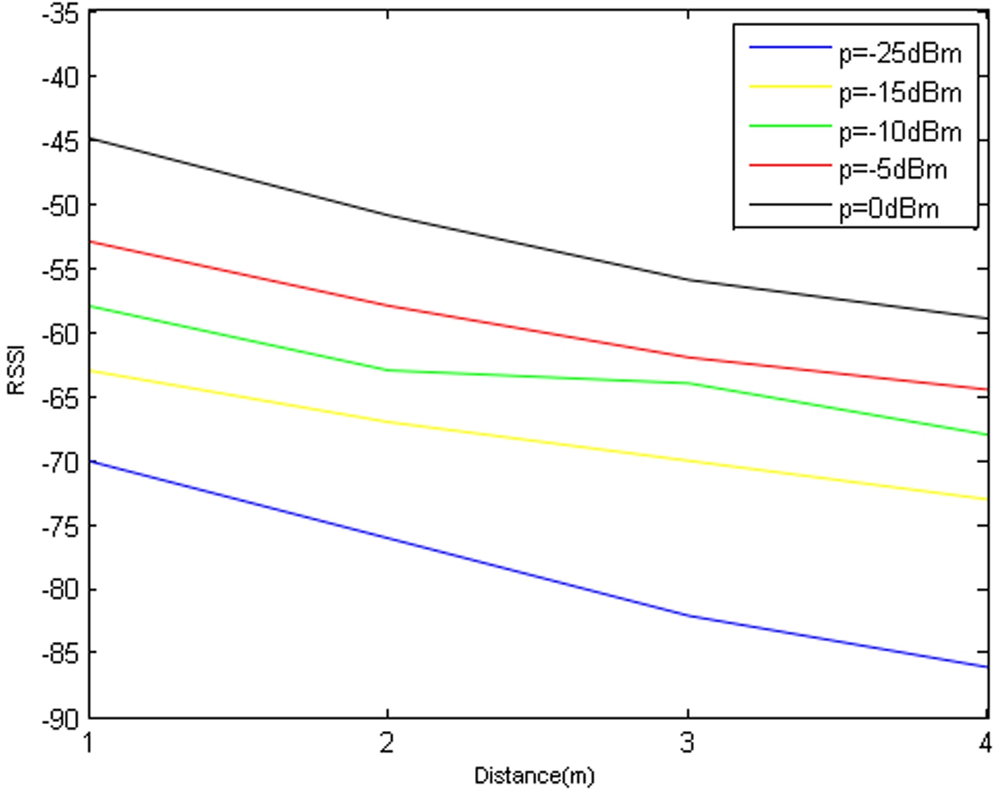
Figure 8.

An RSSI value between sensors under different transmitting powers.

5.2Analyzing and optimizing RSSI measurements

The wireless signal is always disturbed by unstable factors in practical applications. When the distance between nodes increases to a certain extent, the intensifying interferences of radio signals make RSSI measurements appear to jump. At this point, the error is serious and the measured RSSI becomes an invalid value. Hence, the effect of the working environment on the RSSI and the distance need to be considered In a real context, the sensor deployment and the output power of the transmitter will influence RSSI accuracy.

Therefore, two significant analyses are performed under different conditions to improve RSSI accuracy. First, the transmitting power of the RSSI transmitter is set to its highest level (0 dBm), the height of the transmitter and receiver is adjusted, and the meaningful range of RSSI values is analyzed when the distance between transmitter and receiver is varied. Second, the height of the RSSI transmitter and receiver is set to 0.8 m above the ground, the transmitting power is adjusted, and the relationship between the RSSI values and the distance is figured out. One sensor may be picked up from four wearable sensors to receive radio signals.

Table 4

RBLRI algorithm

Algorithm 2. RSSI-based left or right identification
1.	Initialize.
2.	Set RSSI transmitters to periodically transmit a broadcast message to wearable sensors under the selected transmitting
	power.
3.	Calculate the RSSI value of each sensor using the received messages from the nearer RSSI transmitter.
4.	Calculate the horizontal locations of sensors by performing the two-sample t tests.

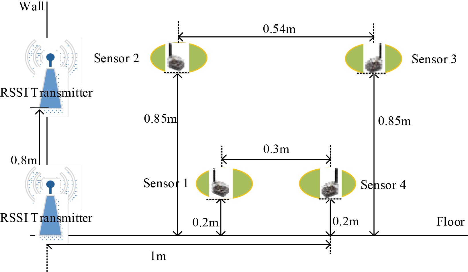
5.2.1Sensor deployment

The core of the experiment is to determine the relationship between RSSI and distance under different deployment rules. At each distance d, 100 RSSI values, which are then averaged to calculate the recorded RSSI. Height interval is 0.5 m, and the highest height is 1.5 m. The relationship between RSSI and distance is obtained by repeating the aforementioned step, as shown in Fig. 7.

Generally, the RSSI attenuation increases with distance. The attenuation increases fast as the distance increases from 1 to 2 m, when the transmitter and receiver are simultaneously placed at a height h (h= 0, 0.5, or 1 m) above the floor. Especially, the attenuation increases rapidly when the height increases from 0 to 0.5 m. This is because when the transmitter and receiver are both placed on the floor, almost all the received signals are reflected, the signal propagation delays are larger, and the attenuations of the received signals are comparatively strong. As the deployment height increases, the attenuation becomes gentler.

Moreover, RSSI values will show an attenuation trend as distance increases, but it dodoes not extremely decrease progressively. In Fig. 7, the relationship between RSSI and distance is not a rigid straight line, as there is a degree of fluctuation. The closer the transmission distance, the faster the decrease in RSSI value, causing a larger difference of RSSI between the left and right the limbs. This contributes to distinguishing which sensor is placed on which limb. Therefore, RSSI values can obtain a higher accuracy in shorter distances.

Table 5

Comparison of means and standard deviations in three sensor deployments

Sensor	First deployment		Second deployment		Third deployment
	M (dBm)	SD	M (dBm)	SD	M (dBm)	SD
Sensor 1	-40.41	0.49	-46.35	1.24	-40.41	0.49
Sensor 2	-46.99	0.73	-41.93	0.79	-41.93	0.79
Sensor 3	-47.53	3.02	-47.58	1.07	-47.58	1.07
Sensor 4	-49.04	0.80	-46.71	3.25	-49.04	0.80

Table 6

Comparison of the significant differences among three deployments

Group	Sensor	First deployment			Second deployment			Third deployment
		Δ⁢P	Δ⁢P(95%CI)	P	Δ⁢P	Δ⁢P(95%CI)	P	Δ⁢P	Δ⁢P(95%CI)	P
		(dBm)	(dBm), (dBm)		(dBm)	(dBm), (dBm)		(dBm)	(dBm), (dBm)
1	Sensor 1	8.63	8.44, 8.81	0.00	0.36	-0.33, 1.05	0.30	8.63	8.44, 8.81	0.00
	Sensor 4
2	Sensor 2	0.54	-0.08, -1.16	0.09	5.65	5.39, 5.91	0.00	5.65	5.39, 5.91	0.00
	Sensor 3

5.2.2Transmitting power

Transmission tests are performed to understand the meaningful range of RSSI under different transmitting powers. The recorded RSSI is also given the average of 100 times for test data. For various power levels (0, 1, 2, 3, 6, 9, 15, 21, 27 and 31) equal to (-25, -20, …, 0 dBm) [23], tests are performed in an indoor environment. The RSSI transmitter is placed at a height of 0.8 m above the floor.

As illustrated in Fig. 8, when the sensor transmitting power is -25 or 0 dBm, the RSSI attenuation increases fast as the distance increases. When the sensor transmitting power is from -5 to -15 dBm, the attenuation increases moderately with the increasing distance. However, a lower transmission power may result in a high packet loss.

The relationship between RSSI and distance conforms to the channel model. When sensors have a short distance, the RSSI attenuation is linear. Conversely, when the distance between sensors increases to a certain extent, the RSSI is affected by a large disturbance. At this point, the calculated distance error is serious. The uncertainty of RSSI increases as the receiver moves further away from the transmitter. Therefore, RSSI values can obtain a higher accuracy in shorter distances. The RBLRIRBLRI algorithm is described in Table 4.

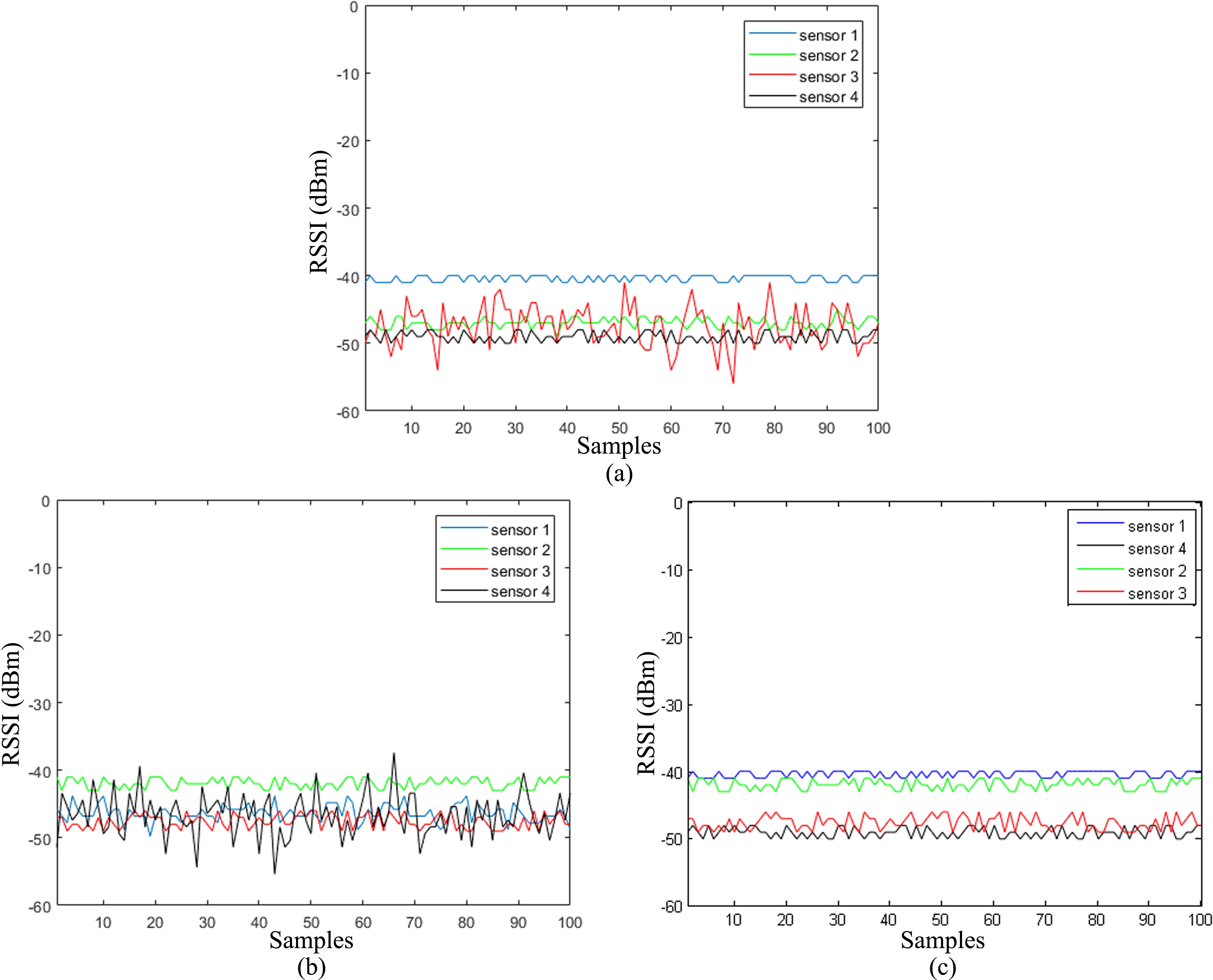
Figure 9.

RSSI measurements under different sensor deployments. (a) Two RSSI transmitters are placed on the floor. (b) Two RSSI transmitters are placed at a height of 0.8 m above the floor. (c) One transmitter on the floor and the other one at a height of 0.8 m above the floor.

5.3RSSI measurement and results

From the aforementioned BAV experiment, both sensors 1 and 4 are the leg nodes and sensors 2 and 3 are the wrist nodes. Hence, the RSSI difference between sensors 1 and 4, and between sensors 2 and 3 need to be considered.

Extensive simulations were performed under different conditions to evaluate the performance of BAV. First, the results from different sensor deployments were compared and analyzed. Then, the identification results under different transmitting powers were compared. Every experiment collects 100 RSSI measurements in each wearable sensor. The transmitting power of the RSSI transmitter is set to 0 dBm.

Figure 9 indicates the RSSI measurements for three sensor deployments. Sensor 3 in Fig. 9a and sensor 4 in Fig. 9b have a larger fluctuation. This is consistent with the aforementioned idea that the farther the transmission distance is from the transmitter to the receiver, the more the RSSI fluctuates. Moreover, the body interference might be also a reason.

Subsequently, the mean M and SD of RSSI reading among three sensor deployments are investigated, as shown in Table 5. In the first deployment, sensor 3 has a larger SD, and in the second deployment, sensor 4 has also a larger SD, consistent with the aforementioned analysis.

The significant difference among three sensor deployments is compared through two-sample t tests, to accurately determine the horizontal position of sensors, as shown in Table 6. The third deployment outperforms other deployments in terms of identification accuracy.

Table 6 reveals that in the first deployment, the P value of group 2 is above 0.05, and in the second deployment, the P value of group 1 is also above 0.05. This indicates that the data cannot be used to statistically reject sensors 2 and 3 at different locations. The same can be concluded for sensors 1 and 4 in the second deployment.

In the third deployment, group 1 (between sensors 1 and 4) has an RSSI difference measurement of 8.63 dBm on an average, with a measured difference of 8.44–8.81 dBm with a 95% CI; group 2 (between sensors 2 and 3) has an RSSI has different measurement of 5.65 dBm an average, with a measured difference of 8.44–8.81 dBm with a 95% CI. Moreover, two-sample t tests return P values of 0 for two groups, demonstrating that the RSSI measurement of sensor 1 is statistically different from that of sensor 4, and the RSSI of sensor 2 is statistically different from that of sensor 3, with > 99.9% CI. These results strongly imply that the values from sensor 1 differ sufficiently from sensor 4 to enable the identification of the horizontal locations of sensors, on the basis of the theory that the lower the RSSI value, the longer the distance.

Table 7

Comparison of means and standard deviations among the three transmitting powers

Sensor	0 (dBm)		-5 (dBm)		-10 (dBm)
	M (dBm)	SD	M (dBm)	SD	M (dBm)	SD
Sensor 1	-40.41	0.49	-51.02	0.67	-56.69	0.53
Sensor 2	-41.93	0.79	-49.12	0.87	-53.87	0.77
Sensor 3	-47.58	1.07	-53.26	1.11	-57.92	1.05
Sensor 4	-49.04	0.80	-51.25	0.88	-56.87	0.86

Table 8

Comparison of significant differences among the three transmitting powers

Group	Sensor	0 (dBm)			-5 (dBm)			-10 (dBm)
		Δ⁢P	Δ⁢P(95%CI)	P	Δ⁢P	Δ⁢P(95%CI)	P	Δ⁢P	Δ⁢P(95%CI)	P
		(dBm)	(dBm), (dBm)		(dBm)	(dBm), (dBm)		(dBm)	(dBm), (dBm)
1	Sensor 1	8.63	8.44, 8.81	0.00	0.23	0.01, 0.45	0.04	0.18	-0.02, 0.38	0.08
	Sensor 4
2	Sensor 2	5.65	5.39, 5.91	0.00	4.14	3.86, 4.42	0.00	4.05	3.79, 4.31	0.00
	Sensor 3

Figure 10.

The proposed setup.

Therefore, sensor 1 is the right leg node, sensor 2 is the right wrist node, sensor 3 is the left wrist node, and sensor 4 is the left leg node. The proposed setup is illustrated in Fig. 10.

Besides, the performance of RBLRI is examined using three transmitting powers. The 0, -5 and -10 dBm transmitting powers are considered. The sensor deployment is set to the optimal model where one RSSI transmitter is placed on the floor and the other one at a height of 0.8 m, 8 m above the floor.

Figure 11.

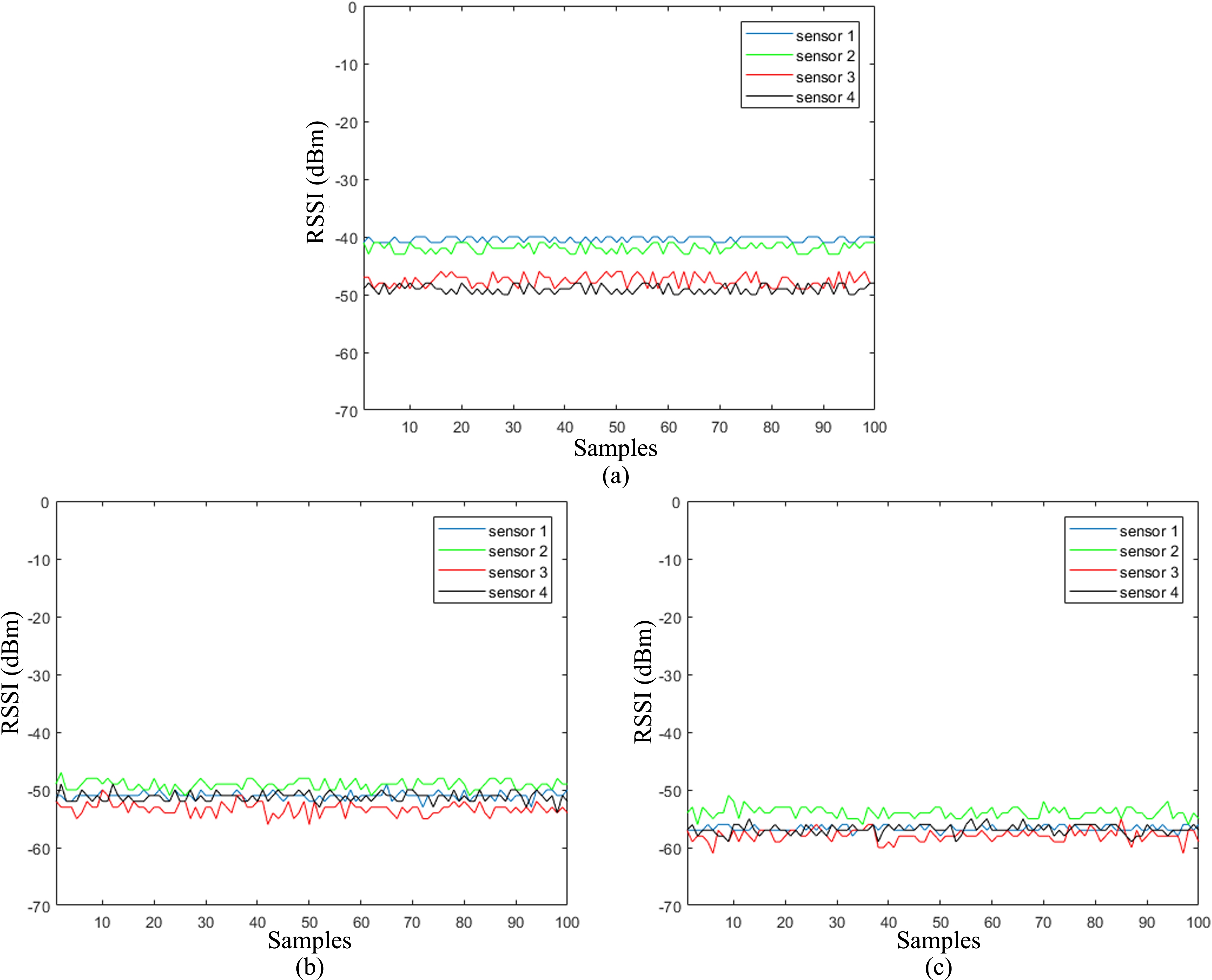
RSSI measurements of four sensors under transmitting powers. (a) The 0 dBm transmitting power. (b) The -5 dBm transmitting power. (c) The -10 dBm transmitting power.

Figure 11 indicates the RSSI measurements for three sensor deployments. All RSSI measurements are quite close in the -10 dBm transmitting power. This observation is also not surprising as the lower the transmitting power, the slower the decrease in the RSSI measurement.

The M and SD of RSSI readings among three transmitting powers are investigated. Table 7 reveals that the RSSI difference of the 0 dBm transmitting power is greater than others, contributing to locating the position of the sensor. For instance, in 0 dBm transmitting power, the difference of mean is 8.63, which for the -5 dBm and -10 dBm transmitting powers are 4.14 and 4.05, respectively.

Further, the significant difference among three transmitting powers through two-sample t tests, is compared to investigate the effectiveness of RBLRI, as presented in Table 8. Clearly, the performance in the 0 dBm transmitting power outperforms others in terms of identification accuracy.

Table 8 reveals that in the -10 dBm transmitting power, the P value of group 1 is above 0.05. This means that the data cannot be used to statistically reject sensors 1 and 4 at different locations. Moreover, in the -5 dBm transmitting power, a larger P value is obtained. This indicates that RSSI measurements are fairly close, insufficient to differentiate the location of the senor.

6.Conclusion and future work

Sensor misplacement could obtain the inconsistent data with the desired patterns at the designated location. This study proposes a new scheme to enable WBANs to instantly recognize which wearable sensor is placed on which limb of the patient. Hypsometry information is employed in the air pressure distribution to determine the vertical location of the wearable sensors. Moreover, the present study demonstrates the meaningful range of the RSSI for identifying the horizontal positions of wearable sensors. To validate the proposed scheme, comprehensive statistical analyses are conducted. This scheme is applicable to home-based old people and patients with tremors or dyskinesia symptoms without the help of the caregiver.

The most important steps, which should be further investigated in the future, are to test the proposed scheme in a large-scale study and expand the types of contextual information from wearable sensors, for instance, by adding heart rate sensors to further monitor body states.

Acknowledgments

The work was supported by the National High Technology Research and Development Program of China (Grant No. 2015AA016005), the National Natural Science Foundation of China (Grant No. 61402096), and China Postdoctoral Science Foundation (Grant No. 2016M591448).

Conflict of interest

None to report.

References

[1]	Savita S, Shruti V, Chakarvarti SK. A review on wireless body area network (WBAN) for health monitoring system: Implementation protocols. Communications on Applied Electronics (2016) ; 4: (7): 16-20.
[2]	Kachroo R, Bajaj DRR. A novel technique for optimized routing in wireless body area network using genetic algorithm. Journal of Network Communications and Emerging Technologies (JNCET) (2015) ; 2: (2).
[3]	Hanson MA, Powell HC, Jr., Barth AT, et al. Body area sensor networks: Challenges and opportunities. Computer (2009) ; (1): 58-65.
[4]	Movassaghi S, Abolhasan M, Lipman J, et al. Wireless body area networks: A survey. Communications Surveys and Tutorials, IEEE (2014) ; 16: (3): 1658-1686.
[5]	Mistry HP, Mistry NH. RSSI based localization scheme in wireless sensor networks: A survey. Proceedings of the 2015, Fifth International Conference on Advanced Computing and Communication Technologies, IEEE (2015) ; 647-652.
[6]	Cotton SL, D’Errico R, Oestges C. A review of radio channel models for body centric communications. Radio Science (2014) ; 49: (6): 371-388.
[7]	Shaban HA, El-Nasr MA, Buehrer RM. Toward a highly accurate ambulatory system for clinical gait analysis via UWB radios. Information Technology in Biomedicine, IEEE Transactions on (2010) ; 14: (2): 284-291.
[8]	Kavitha MG, SendhilNathan S. Body area network with mobile anchor based localization. Cluster Computing (2017) ; 1-10.
[9]	Bharadwaj R, Swaisaenyakorn S, Parini CG, et al. Impulse radio-ultra wideband communications for localisation and tracking of human body and limbs movement for healthcare applications. IEEE Transactions on Antennas and Propagation (2017) .
[10]	Yessad N, Bouchelaghem S, Ouada FS, et al. Secure and reliable patient body motion based authentication approach for medical body area networks. Pervasive and Mobile Computing (2017) .
[11]	Vahdatpour A, Amini N, Sarrafzadeh M. On-body device localization for health and medical monitoring applications. Proceedings of the 2011, IEEE International Conference on Pervasive Computing and Communications, IEEE (2011) ; 37-44.
[12]	Lo G, González-Valenzuela S, Leung VCM. Automatic identification and placement verification of wearable wireless sensor nodes using atmospheric air pressure distribution. Consumer Communications and Networking Conference (CCNC), IEEE (2012) ; 32-33.
[13]	Luo Q, Peng Y, Li J, et al. RSSi-based localization through uncertain data mapping for wireless sensor networks. IEEE Sensors Journal (2016) ; 16: (9): 3155-3162.
[14]	Awad A, Frunzke T, Dressler F. Adaptive distance estimation and localization in WSN using RSSI measures. Proceedings of the 10th, Euromicro Conference on Digital System Design Architectures, Methods and Tools, IEEE (2007) ; 471-478.
[15]	Huo L. Research of barometric altimeter and the method accuracy. J PLA Inst Surv Mapp (2002) ; 22: (2): 21-25.
[16]	Sheng PX, Mao JT, Li JG, et al. Atmospheric physics. Peking University press (2003) . p. 84-99.
[17]	Gharghan SK, Nordin R, Ismail M, et al. Accurate wireless sensor localization technique based on hybrid PSO-ANN algorithm for indoor and outdoor track cycling. IEEE Sensors Journal (2016) ; 16: (2): 529-541.
[18]	Minghui Z, Huiqing Z. Research on model of indoor distance measurement based on receiving signal strength. Proceedings of the 2010, International Conference on Computer Design and Applications (ICCDA), IEEE (2010) ; 5: : V5-54-V5-58.
[19]	Qi Y. Wireless geolocation in a non-line-of-sight environment, Ph.D. dissertation, Princeton Univ; Princeton, NJ: (2003) .
[20]	Zhu H, Alsharari T. An improved RSSI-based positioning method using sector transmission model and distance optimization technique. International Journal of Distributed Sensor Networks (2015) ; 187.
[21]	Shin M, Joe I. An indoor localization system considering channel interference and the reliability of the RSSI measurement to enhance location accuracy. Proceedings of the 17th, International Conference on Advanced Communication Technology (ICACT), IEEE (2015) ; 583-592.
[22]	Dieng NA, Chaudet C, Charbit M, et al. Experiments on the RSSI as a Range Estimator for Indoor Localization. Proceedings of the 5th, International Conference on New Technologies, Mobility and Security (NTMS), IEEE (2012) ; 1-5.
[23]	Cong L. Research on privacy protection algorithm in wireless body area network. Northeastern University; (2015) .