
Learning SHACL shapes from knowledge graphs
Abstract
Knowledge Graphs (KGs) have proliferated on the Web since the introduction of knowledge panels to Google search in 2012. KGs are large data-first graph databases with weak inference rules and weakly-constraining data schemes. SHACL, the Shapes Constraint Language, is a W3C recommendation for expressing constraints on graph data as shapes. SHACL shapes serve to validate a KG, to underpin manual KG editing tasks, and to offer insight into KG structure. Often in practice, large KGs have no available shape constraints and so cannot obtain these benefits for ongoing maintenance and extension.
We introduce Inverse Open Path (IOP) rules, a predicate logic formalism which presents specific shapes in the form of paths over connected entities that are present in a KG. IOP rules express simple shape patterns that can be augmented with minimum cardinality constraints and also used as a building block for more complex shapes, such as trees and other rule patterns. We define formal quality measures for IOP rules and propose a novel method to learn high-quality rules from KGs. We show how to build high-quality tree shapes from the IOP rules. Our learning method, SHACLearner, is adapted from a state-of-the-art embedding-based open path rule learner (Oprl).
We evaluate SHACLearner on some real-world massive KGs, including YAGO2s (4M facts), DBpedia 3.8 (11M facts), and Wikidata (8M facts). The experiments show that our SHACLearner can effectively learn informative and intuitive shapes from massive KGs. The shapes are diverse in structural features such as depth and width, and also in quality measures that indicate confidence and generality.
1.Introduction
While public knowledge graphs (KGs) became popular with the development of DBpedia [2] and Yago [33] more than a decade ago, interest in enterprise knowledge graphs [26] has taken off since the inclusion of knowledge panels on the Google Search engine in 2012, driven by its internal knowledge graph. Although these KGs are massive and diverse, they are typically incomplete. Regardless of the method that is used to build a KG (e.g., collaboratively vs individually, manually vs automatically), it will be incomplete because of the evolving nature of human knowledge, cultural bias [7] and resource constraints. Consider Wikidata [35], for example, where there is more complete information for some types of entities (e.g., pop stars), while less for others (e.g., opera singers). Even for the same type of entity, for example, computer scientists, there are different depths of detail for similarly accomplished scientists, depending on their country of residence.
However, the power of KGs comes from their data-first approach, enabling contributors to extend a KG in a relatively arbitrary manner. By contrast, a relational database typically employs not-null and other schema-based constraints that require some attributes to be instantiated in a defined way at all times. Large KGs are typically populated by automatic and semi-automatic methods using non-structured sources such as Wikipedia that are prone to errors of omission (i.e., incompleteness) and commission (i.e., falsity). Both kinds of errors can be highlighted for correction by a careful application of schema constraints. However, such constraints are commonly unavailable and, if available, uncertain and frequently violated in a KG for valid reasons, arising from the intended data-first approach of KG applications.
SHACL [21] was formally recommended by the W3C in 2017 to express such constraints on a KG as shapes. For example, SHACL can be used to express that a person (in a specific use case) needs to have a name, birth date, and place of birth, and that these attributes have particular types: a string; a date; and a location. The shapes are used to guide the population of a KG, although they are not necessarily enforced. Typically, SHACL shapes are manually-specified. However, as for multidimensional relational database schemes [19], shapes could, in principle, be inferred from KG data. As frequent patterns, the shapes characterise a KG and can be used for subsequent data cleaning or ongoing data entry. There is scant previous research on this topic [4,5,14,16,23,31].
While basic SHACL [21] and its advanced features [20] allows the modelling of diverse shapes including rules and constraints, most of these shapes are previously well known when expressed by alternative formalisms, including closed rules [15], trees, existential rules [3], and graph functional dependencies [13]. We claim that the common underlying form of all these shapes is the path, over which additional constraints induce alternative shapes. For example, in DBpedia we see the following path,
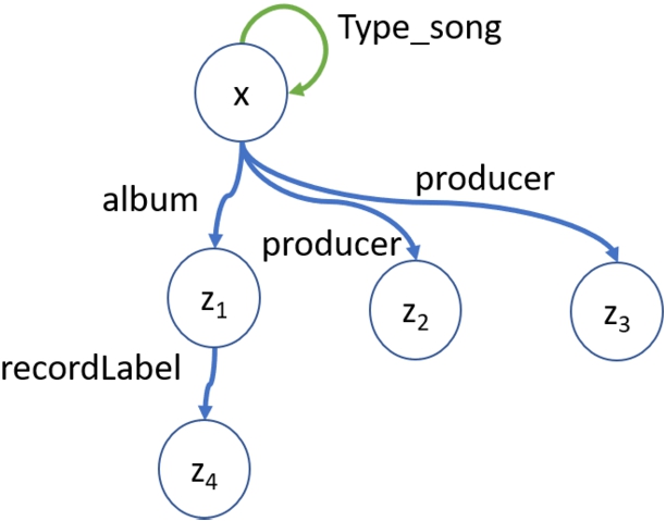
Since the satisfaction of a less-constrained shape is a necessary condition for satisfaction of a more complex shape (but not a sufficient condition), in this paper we focus on learning paths, the least constrained shape for our purposes. In addition, we learn cardinality constraints that can express, for example, that a song has at least 2 producers. We also investigate the process of constructing one kind of more complex shape, that is a tree, out of paths. For example, we discover a tree about an entity which has song as its type as shown in Fig. 1. In a KG context, the tree suggests that if we have an entity of type song in the KG, then we would expect to have the associated facts too.
Fig. 1.
A tree shape for the Song concept from DBpedia.
In this paper, we present a system, SHACLearner, that mines shapes from KG data. For this purpose we propose a predicate calculus formalism in which rules have one body atom and a chain of conjunctive atoms in the head with a specific variable binding pattern. Since these rules are an inverse version of open path rules [18], we call them inverse open path (IOP) rules. To learn IOP rules we adapt an embedding-based open path rule learner, Oprl [18]. We define quality measures to express the validity of IOP rules in a KG. SHACLearner uses the mined IOP rules to subsequently discover more complex tree shapes. Each IOP rule or tree is a SHACL shape, in the sense that it can be syntactically rewritten in SHACL. Our mined shapes are augmented with a novel numerical confidence measure to express the strength of evidence in the KG for each shape.
In summary, the main contributions of this paper are:
– We introduce a new formalism called Inverse Open Path rules, that serves as a building block for more complex shapes such as trees, together with cardinality constraints and quality measurements;
– We extend the Open Path rule learning method, Oprl [17,18], to learn IOP (Inverse Open Path) rules annotated with cardinality constraints, while introducing unary predicates that can act as class or type constraints; and
– We propose a method to aggregate IOP rules to produce tree shapes.
2.Preliminaries
The presentation of closed path rules and open path rules in this section is adapted and extended from [18].
An entity e is an identifier for an object such as a place or a person. A fact (also known as a link) is an RDF triple
2.1.Closed-path rules
KG rule learning systems employ various rule languages to express rules. RLvLR [27] and ScaleKB [9] use so-called closed path (CP) rules. Each consists of a head at the front of the implication arrow and a body at the tail. We say the rule is about the predicate of the head. The rule forms a closed path, or single unbroken loop of links between the variables. It has the following general form.
We interpret these kinds of rules with universal quantification of all variables at the outside, and so we can infer a fact that instantiates the head of the rule by finding an instantiation of the body of the rule in the KG. For example, from the rule
Rules are considered of more use if they generalise well, that is, they explain many facts. To quantify this idea we recall measures support, head coverage and standard confidence that are used in some major approaches to rule learning including [9] and [15].
Definition 1
Definition 1(satisfies, support).
Let r be a CP rule of the form (1). A pair of entities
Standard confidence (SC) and head coverage (HC) offer standardised measures for comparing rule quality. SC describes how frequently the rule is true, i.e., of the number of entity pairs that satisfy the body in the KG, what proportion of the inferred head instances are satisfied? It is closely related to confidence widely used in association rule mining [1]. HC measures the explanatory power of the rule, i.e., what proportion of the facts satisfying the head of the rule could be inferred by satisfying the rule body? It is closely related to cover which is widely used for rule learning in inductive logic programming [34]. A non-recursive rule that has both 100% SC and HC is redundant with respect to the KG, and every KG fact that is an instance of the rule head is redundant with respect to the rule.
Definition 2
Definition 2(standard confidence, head coverage).
Let
2.2.Open-path rules: Rules with open variables
Unlike earlier work in rule mining for KG completion, Oprl for active knowledge graph completion [18] defines open path (OP) rules of the form:
We call a variable closed if it occurs in at least two distinct predicate terms, such as
To assess the quality of OP rules, we use open path standard confidence (OPSC) and open path head coverage (OPHC) which are derived in [18] from the closed path forms (Definition 2).
Definition 3
Definition 3(open path: OPsupp, OPSC, OPHC).
Let r be an OP rule of the form (2). Then a pair of entities
2.3.SHACL shapes
A KG is a schema-free database and does not need to be augmented with schema information natively. However, many KGs are augmented with type information that can be used to understand and validate data and can also be very helpful for inference processes on the KG. In 2017 the Shapes Constraint Language (SHACL) [21] was introduced as a W3C recommendation to define schema information for KGs stored as an RDF graph. SHACL defines constraints for graphs as shapes. KGs can then be validated against a set of shapes.
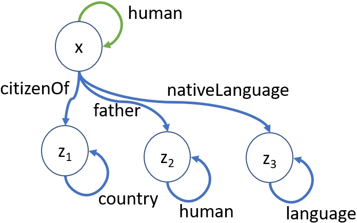
Shapes can serve two main purposes: validating the quality of a KG and characterising the frequent patterns in a KG. In Fig. 2, we illustrate an example of a shape from Wikidata,11 where x and
humanShape
    a sh:NodeShape;
    sh:targetClass class:human ;
    sh:property [
        sh:path property:citizenOf ;
        sh:class class:country ;
        sh:nodeKind sh:IRI ;
    ];
    sh:property [
        sh:path property:father ;
        sh:class class:human ;
        sh:nodeKind sh:IRI ;
    ];
    sh:property [
        sh:path property:nativeLanguage ;
        sh:class class:language ;
        sh:nodeKind sh:IRI ;
    ];
SHACL, together with SHACL advanced features [20] is extensive. Here we focus on the core of SHACL in which node shapes constrain a target predicate (e.g., the unary predicate
Fig. 2.
An example of a SHACL shape from Wikidata.
Various formalisms with corresponding shapes have been proposed to express diverse kinds of patterns exhibited in KGs, such as k-cliques, Closed rules (CR) [15] (that include closed path rules), Functional Graph Dependency (FGD) [13], and trees [3]. CRs are used for inferring new facts. FGDs define constraints like the type of entities in the domain and range of predicates, or the number of entities to which an entity can be related by a specific predicate. These constraints are deployed to make the KG consistent. Regardless of differences amongst these formalisms, they share a key feature in their syntax. The building block for expressing all of these shape constraints is a sequence of predicates.
We focus on such path shapes for our shape learning system. A path is a sequence of predicates connected by closed intermediate variables but terminating with open variables at both ends. Although shapes in the form of a path are less constrained than some more complex shapes, they are a more general template for more complex shapes like closed rules or trees, which are also paths (with further restrictions). We will define Inverse Open Path rules induced from paths that have a straightforward interpretation as shapes, and also propose a method to mine such rules from a KG. To demonstrate the potential for these kind of shapes to serve as building blocks for more complex shapes, we then propose a method that builds trees out of mined rules, and briefly discuss the application of such trees to KG completion.
3.SHACL learning
3.1.Rules with open variables or uncertain shapes
We observe that the converse of OP rules, that we call inverse open path rules (IOP), correspond to SHACL shapes. For example, the shape of Fig. 2 can be derived from the following three IOP rules:
To assess the quality of IOP rules we follow the style of quality measures for OP rules [18].
Definition 4
Definition 4(inverse open path: IOPsupp, IOPSC, IOPHC).
Let r be an IOP rule of the form (3). Then a pair of entities
Notably, because any instantiated open path in a KG induces both an OP and IOP rule: the support for an IOP rule is the same as the support for its corresponding OP form; IOPSC is the same as the corresponding OPHC; and IOPHC is the same as the corresponding OPSC. This close relationship between OP and IOP rules helps us to mine both OP and IOP rules in the one process.
We show the relationship between an OP rule and its converse IOP version in the following example. Consider the OP rule,
In many cases we need the rules to express not only the necessity of a chain of facts (the facts in the head of the IOP rule) but the number of different chains which should exist. For example, we may need a rule to express that each human has at least two parents. Hence, we introduce IOP rules annotated with a cardinality,
Definition 5
Definition 5(Cardinality of an IOP rule, Car).
Let r be an annotated IOP rule of the form (4) and let
The cardinality expresses a lower bound on the number of head paths which are satisfied in the KG for every instantiation of the variable that joins the body to the head. For example, if we have
Rules with the same head and the same body may have different cardinalities. In the given example we might have the following rule as well,
Lemma 1
Lemma 1(IOPSC is non-increasing with length).
Let r be an IOP rule of the form (3) with
Proof.
Observe that by Definition 4, the denominator of
This Lemma is useful in the process of rule learning since it shows that if we discard a rule due to its low IOPSC, v, we do not need to check the rule extended with more head atoms, since those rules’ IOPSCs are at most v. Hence the process of pruning such rules does not harm the completeness of the rule learning.
3.2.IOP learning through representation learning
To mine IOP rules, we start with the open path rule learner Oprl [18], and adapt its embedding-based OP rule learning to learn annotated IOP rules. We call this new IOP rule learner, SHACLearner, shown in Algorithm 1.
SHACLearner uses a sampling method
While the overall algorithm structure of SHACLearner is similar to Oprl [18], as is the embedding-based scoring function, the following elements are novel in SHACLearner:
– Oprl cannot handle unary predicates while SHACLearner admits unary predicates both in the head and the body of IOP rules.
– SHACLearner can discover and evaluate IOP rules with minimum cardinality constraints in the head of the IOP rule, while Oprl is effectively limited to learning the special case of minimum cardinality 1 for all rules. For this reason, the evaluation method of SHACLearner,
– The aggregation module that produces trees out of learnt IOP rules, ready for translation to SHACL, is novel in SHACLearner.
Algorithm 1
SHACLearner
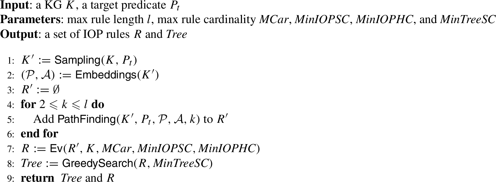
3.3.Sampling
In more detail, the
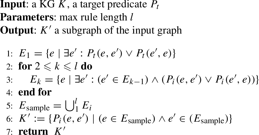
The sampling method, first introduced in [27], is shown in Algorithm 2. Since we search for IOP rules with up to l atoms (including the specific body target predicate,
This simple approach reduces the size of the problem significantly, as discussed in [28]. For a KG K with entities E and facts F, the set of sampled entities for a target predicate will be of size
Algorithm 2
3.4.Embeddings
After sampling, in line 2
Briefly, we use RESCAL [24] to embed each entity
In
3.5.Generating and pruning rules
After that, in line 3 to line 7 of Algorithm 1,
An IOP rule
1. The predicate arguments that have the same variable in the rule should have similar argument emdeddings. For example we should have the following similarities,
2. The whole path forms a composite predicate, like
Based on the above two properties, [18] defines two scoring functions that help us to heuristically mine the space of all possible IOP rules to produce a reduced set of candidate IOP rules.
The ultimate evaluation of an IOP rule will be done in the next step as described below.
3.6.Efficient computation of quality measures
Now we focus our attention on the efficient matrix-computation of the quality measures that are novel for SHACLearner.
Let
We illustrate the computation of IOPSC and IOPHC through an example. Consider the IOP rule
For (1) we can read the pairs
For (2) the pairs
In the example we have
Computing (3) is now straightforward. We have that the row index of non-zero elements of
Hence, we could have three versions of r, i.e.,
3.7.From IOP rules to tree shapes
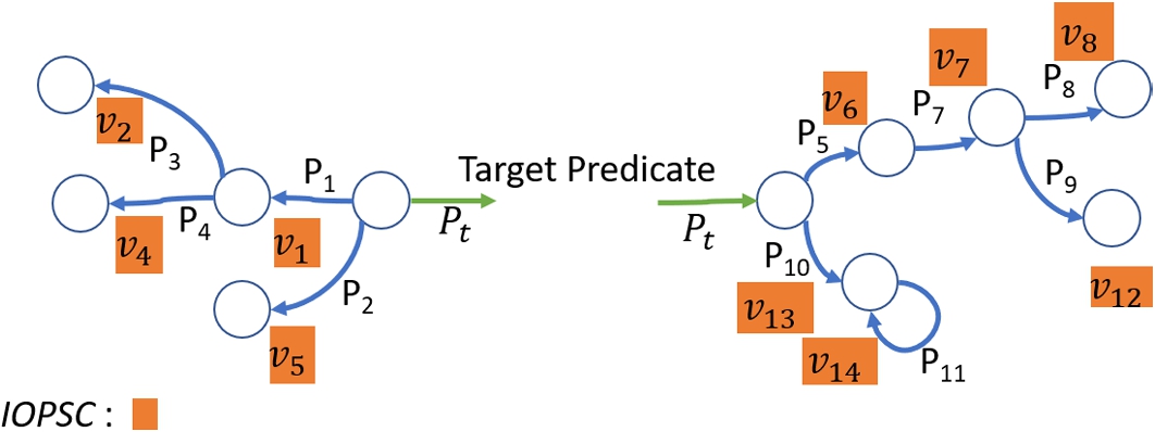
Now in line 8 of Algorithm 1 we turn to deriving SHACL trees, as illustrated in Fig. 3, from annotated IOP rules. This procedure is novel in SHACLearner. We use a greedy search to aggregate the IOP rules for the subject argument and the object argument of each target predicate.
For example, the shape of Fig. 2 has the following tree:
To assess the quality of a tree we follow the quality measures for IOP rules.
Definition 6
Definition 6(Tree: Treesupp, TreeSC).
Let r be a tree of the above form. Then a set of pairs of entities
To learn each tree we employ a greedy search,
These uncertain shapes can be presented as standard SHACL shapes by ignoring those that fail to satisfy minimum quality thresholds and deleting the quality annotations. Aside from the cardinality, the tree may be straightforwardly interpreted as a set of SHACL shapes by reading off every path from the target predicate terminating at a node in the tree. The body predicate is declared a sh:nodeShape and the path of head predicates as nested sh:path declarations within a sh:property declaration. Cardinality of a path is read from the annotation of the branch at the terminating node, and declared by sh:minCount within the property declaration. See Section 3.1 for an example.
SHACLearner supports all the SHACL Core22 [21] features (node and property shapes). The limitations of SHACLearner with respect to SHACL Core are: (1) it treats all properties, both object and datatype properties, as “plain predicates” so there is no distinction; (2) and so it does not perform any kind of data type validation; and (3) of cardinality expressions, only min cardinality is handled. SHACLearner does not mine SPARQL-like constraints, SHACL-SPARQL.33
Fig. 3.
Trees for a target predicate
3.7.1.Tree shapes are useful for human interaction
Shapes offer KG documentation as readable patterns and also provide a way to validate a KG. Our novel tree shapes can additionally be used for KG-completion. While there are several methods proposed to complete KGs automatically (e.g., [24,25,27]) by predicting missing facts (also called links), all these methods traverse the KG in a breadth-first manner. In other words, they sequentially answer a set of independent questions such as
Tree shapes can also help a human expert to extract a more intuitive concise sub-tree out of a deeper, more complex tree when desired for human interpretation. If a tree with confidence
4.Related work
There are some exploratory attempts to address learning SHACL shapes from KGs [4,14,16,23,31]. They are procedural methods without logical foundations and are not shown to be scalable to handle real-world KGs. They work with a small amount of data and the representation formalism they use for their output is difficult to compare with the IOP rules which we use in this paper. [4] carries out the task in a semi-automatic manner: it provides a sample of data to an off-the-shelf graph structure learner and provides the output in an interactive interface for a human user to create SHACL shapes.
In [5] the authors provide an interactive framework to define SHACL shapes with different complexities, including nested patterns that are similar to the trees that we use. A formalisation of the approach is given, but there are no shape quality measures that are essential for large scale shape mining. Because the paper does not provide a system that discovers patterns from massive KGs, we cannot deploy their method for comparison purposes.
There are some works [10,29] that use existing ontologies for KGs to generate SHACL shapes. [10] uses two different kinds of knowledge to automatically generate SHACL shapes: ontology constraint patterns as well as input ontologies. In our work we use the KG itself to discover the shapes, without relying on external modelling artefacts.
From an application point of view, there are papers which investigate the application of SHACL shapes to the validation of RDF databases including [6,22], but these do not contribute to the discovery of shapes.
[30] proposes an extended validation framework for the interaction between inference rules and SHACL shapes in KGs. When a set of rules and shapes are provided, a method is proposed to detect which shapes could be violated by applying a rule.
There are some attempts to provide logical foundations for the semantics of the SHACL language including [11] that presents the semantics of recursive SHACL shapes. By contrast, in our work we approach SHACL semantics in the reverse direction. We start with logical formalisms with both well-defined semantics and motivating use cases to derive shapes that can be trivially expressed in a fragment of SHACL.
5.Experiments
We have implemented our SHACLearner44 based on Algorithm 1, and conducted experiments to assess it. Our experiments are designed to prove the effectiveness of our SHACLearner at capturing shapes with varying confidence, length and cardinality from various real-world massive KGs. Since our proposed system is the first method to learn shapes from massive KGs automatically, we have no benchmark with which to compare. However, the performance of our system shows that it can handle the task satisfactorily and can be applied in practice. We demonstrate that:
1. SHACLearner is scalable so it can handle real-world massive KGs including DBpedia with over 11M facts.
2. SHACLearner can learn several shapes each for various target predicates.
3. SHACLearner can discover diverse shapes with respect to the quality measurements of IOPSC and IOPHC.
4. SHACLearner discovers shapes of varying complexity, and diverse with respect to length and cardinality.
5. SHACLearner discovers every high-quality rule (with
6. SHACLearner discovers more complex shapes (trees) by aggregating learnt IOP rules efficiently.
Our four benchmark KGs are described in Table 1. Three benchmarks, namely YAGO2s, Wikidata, and DBpedia, are common KGs and have been used in rule learning experiments previously [15,27]. The fourth is a small synthetic KG, Poker, for analysing the completeness of our algorithm. The Poker KG was introduced in [18], adapted from the classic version [8,12] to be a rich and correct KG for evaluation experiments. Each poker hand comprises 5 playing cards drawn from a deck with 13 ranks and 4 suits. Each card is described using two attributes: suit and rank. Each hand is assigned to any or all of 9 different ranks, including High Card, One Pair, Two Pair, etc. We randomly generate 500 poker hands and all facts related to them to build a small but complete and correct KG as summarised in Table 1. 28 out of 35 predicates are unary predicates, such as
Table 1
Benchmark specifications
| KG | # Facts | # Entities | # Predicates |
| YAGO2s | 4,122,438 | 2,260,672 | 37 |
| Wikidata | 8,397,936 | 3,085,248 | 430 |
| Wikidata +UP | 8,780,716 | 3,085,248 | 587 |
| DBpedia 3.8 | 11,024,066 | 3,102,999 | 650 |
| DBpedia 3.8 +UP | 11,498,575 | 3,102,999 | 1,005 |
| Poker | 6, 790 | 575 | 35 |
All experiments were conducted on an Intel Xeon CPU E5-2650 v4 @2.20 GHz, 66GB RAM and running CentOS 8.
5.1.Transforming KGs with type predicates for experiments
Since real-world KG models treat predicates and entities in a variety of ways, we require a common representation for this work that clearly distinguishes entities and predicates. We employ an abstract model that is used in Description Logic ontologies, where classes and types are named unary predicates, and roles (also called properties) are named binary predicates.
Presenting the class and type information as unary predicates also allows us to learn fully abstracted (entity-free) shapes (e.g.
In real-world KGs, concept or class membership may be modeled as entity instances of a binary fact. For example, DBpedia contains “<dbo:type>(
We use the two type-like predicates from DBpedia 3.8 “<dbo:type>” and “<dbo:class>” and the one from Wikidata “<occupation_P106>” to generate our unary predicates and facts. These predicates each have a class as their second argument. To prune the classes with few instances for which learning may be pointless, we consider only our unary predicates which have at least 100 facts. We retain the original predicates and facts in the KG as well as extending it with our new ones. In Table 1 we report the specifications of two benchmarks where we have added the unary predicates and facts (denoted as +UP).
5.2.Learning IOP rules
We follow the established approach for evaluating KG rule-learning methods, that is, measuring the quantity and quality of distinct rules learnt. Rule quality is measured by Inverse open path standard confidence (IOPSC) and Inverse open path head coverage (IOPHC). We randomly select 50 target predicates from Wikidata and DBPedia unary predicates (157 and 355 respectively). We use all binary predicates of YAGO2s (i.e., 37) as target predicates. Each binary target predicate serves as two target predicates, once in the straight form (where the object argument of the predicate is the common variable to connect the head) and secondly in its reverse form (where the subject argument serves to connect). In this manner, we ensure that the results of SHACLearner on YAGO2s with its binary predicates as targets is comparable with the results for Wikidata and DBpedia that have unary predicates as targets. Hence for YAGO2s we have 74 target predicates.
A 10 hour limit is set for learning each target predicate.
Table 2 shows #Rules, the average numbers of quality IOP rules found; %SucTarget, the proportion of target predicates for which at least one IOP rule was found; and the running times in hours, averaged over the targets. Only high quality rules meeting minimum quality thresholds are included in these figures, that is, with IOPSC
Table 2
Performance of SHACLearner on benchmark KGs
| Benchmark | %SucTarget | #Rules | Time (hours) |
| YAGO2s | 80 | 42 | 0.6 |
| Wikidata+UP | 82 | 67 | 1.8 |
| DBpedia+UP | 98 | 157 | 2.4 |
SHACLearner shows satisfactory performance in terms of both the runtime and the numbers of quality rules mined. Note that rules found have a variety of lengths and cardinalities. To better present the quality performance of rules we illustrate the distribution of rules with respect to the features, IOPSC, IOPHC, cardinality and length, and also IOPSC vs length. In the following, the proportion of mined rules having the various feature values is presented, to more evenly demonstrate the quality of performance over the three very different KGs.
Fig. 4.
Distribution of mined rules with respect to IOPSC and IOPHC.
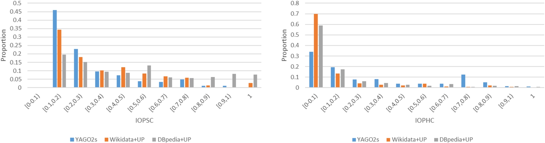
The distribution of mined rules with respect to their IOPSC and IOPHC is shown in Fig. 4. In the left-hand chart we observe a consistent decrease in the proportion of quality rules as the IOPSC increases. In the right hand chart we see a similar pattern for increasing IOPHC, but the decrease is not as consistent, showing there must be many relevant rules with many covered head instances. Over all benchmarks, the majority of learned rules have lower IOPSC and IOPHC. This is expected because the statistical likelihood of poor quality rules is much higher. Indeed, we show experimentally in Section 5.3 that our pruning techniques, that are necessary for scalability, prune away predominantly lower quality rules.
With respect to IOPSC, proportionally more quality rules are learnt from DBpedia than from the other KGs, with Wikidata coming second, ahead of YAGO2s. This phenomenon might be a result of our deliberate selection of type-like unary predicates as targets for DBPedia and Wikidata, whereas for YAGO2s we use every one of the 37 binary predicates as a target.
Fig. 5.
Distribution of mined rules with respect to their cardinalities.
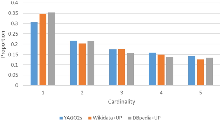
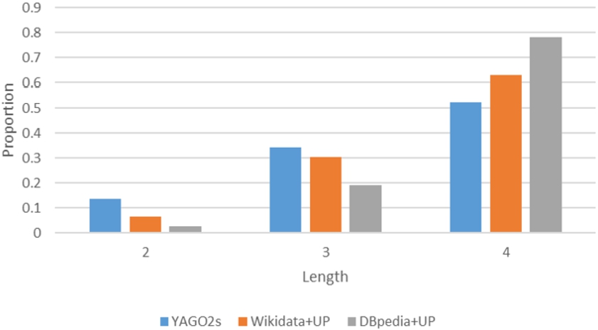
Fig. 6.
Distribution of mined rules with respect to their lengths.
The distribution of mined rules with respect to their cardinalities is shown in Fig. 5. We observe that the largest proportion of rules has a cardinality of 1, as expected, as they have the least stringent requirements to be met in the KG. We observe an expected decrease with greater cardinalities as they demand tighter restrictions to be satisfied. YAGO2 demonstrates a tendency towards higher cardinalities than the other KGs, possibly a result of its more curated development.
The distribution of mined rules with respect to their lengths is shown in Fig. 6. One might expect that as the length increases, the number of rules would increase since the space of possible rules grows, and this is what we see.
For a concrete example of SHACL learning, we show the following three IOP rules mined from DBpedia in the experiments. The IOPSC, IOPHC, and Cardinality annotations respectively prefix each rule.
The rules can be trivially rewritten (through a script that we developed) into SHACL syntax as follows.
:s1 a sh:NodeShape ;
    sh:targetClass :<dbo:type>_<db:Song> ;
    sh:property [
        sh:minCount 1 ;
        sh:path :<dbo:album> ;
            [sh:path :<dbo:recordLabel> ; ]
    ] .
:s2 a sh:NodeShape ;
    sh:targetClass :<dbo:type>_<db:Song> ;
    sh:property [
        sh:minCount 1 ;
        sh:path :<dbo:producer> ;
    ] .
:s3 a sh:NodeShape ;
    sh:targetClass :<dbo:type>_<db:Song> ;
    sh:property [
        sh:minCount 2 ;
        sh:path :<dbo:producer> ;
    ] .
5.2.1.IOPSC vs IOPHC
Using rules found in the experiments, we further illustrate the practical meaning of the IOPSC and IOHC qualities. While IOPSC determines the confidence of a rule based on counting the proportion of target predicate instances for which the rule holds true in the KG, IOPHC indicates the proportion of rule consequent instances that are justified by target predicate instances in the KG, thereby indicating the relevance of the rule to the target. In Wikidata+UP, all unary predicates are occupations such as singer or entrepreneur, so all the entities which have these types turn out to be persons even though there is no explicit person type in our KG. Thus, the occupations all have very similar IOP rules about each of them with high IOPSC and low IOPHC, like the following one, for example.
5.3.Completeness analysis of IOP rule learning
SHACLearner uses two tricks to significantly reduce the search space for IOP rules in
(-S+H): SHACLearner that does not sample and so uses the complete input KG in all components, including embedding learning, heuristic pruning and ultimate evaluation.
(+S-H): SHACLearner that samples but does not use heuristic pruning and so generates rules based on the sampled KG and evaluates rules on the complete KG.
(-S-H): SHACLearner that does not use sampling nor heuristic pruning. This system is an ideal IOP rule learner that generates and evaluates all possible rules up to the maximum length parameter. Since this method is a brute-force search, it cannot handle any real-world KG such as those we used in the performance evaluation (Section 5.2).
(+S+H): SHACLearner with its full functionality.
Table 3
IOPSC performance of the ideal no-pruning SHACLearner variant on Poker, showing the percentage reduction in rules found by IOPSC intervals for variants with sampling and/or heuristic pruning
| Learner/IOPSC | [0.1, 0.3) | [0.3, 0.5) | [0.5, 0.7) | [0.7, 0.9) | [0.9, 1] |
| #(-S-H) | 163 | 44 | 74 | 36 | 46 |
| (-S+H)% | 0% | 0% | |||
| (+S-H)% | 0% | ||||
| (+S+H)% | 0% |
We observe that SHACLearner does not miss any rules of the highest quality, i.e., with
We observe that, unlike the other pruning variants, using heuristic pruning alone in (-S+H) does not uniformly increase in effectiveness with decreasing rule quality. This may be because using the complete KG for learning rules about all target predicates could harm the quality of the learnt embeddings used in the scoring function of SHACLearner. The better quality of embeddings extracted from the sampled KG arises from our sampling method that creates a KG that is customised for the target predicate. All entities in the sampled KG are either directly related to the target predicate or close neighbours of directly related entities as we described in 3.3.
5.4.Learning trees from IOP rules
Now we turn to presenting results for the trees that are built based on the IOP rules discovered in the experiments. We report the characteristics of discovered trees in Table 4. We use a value of 0.1 for the
Table 4
Tree-learning performance of SHACLearner on benchmark KGs
| Benchmark | TreeSC | #branches | Time (hours) |
| YAGO2s | 0.13 | 21 | 0.06 |
| Wikidata+UP | 0.19 | 21 | 0.1 |
| DBpedia+UP | 0.2 | 88 | 0.14 |
The results show the running time for aggregating IOP rules into trees is lower than the initial IOP mining time by a factor greater than 10. If, on the other hand, we wanted to discover such complex shapes from scratch it would be exhaustively time consuming due to the sensitivity of rule learners to the maximum length of rules. The number of potential rules in the search space grows exponentially with the maximum number of predicates of the rules. The average number of branches in the mined trees are 50%, 31%, and 56% of the corresponding number of mined rules respectively from Table 2. Hence, by imposing the additional tree-shaped constraint over the basic IOP-shaped constraint, at least 44% of IOP rules are pruned.
For an example of tree shape learning, in the following, we show a fragment of a 39-branched tree mined from DBpedia by aggregating IOP rules in the experiments.
Here, the first annotation value (0.13) presents the SC of the tree and the subsequent values at the beginning of each branch indicate the branch cardinality. This tree can be read as saying that a song has an album with a record label, an album with two producers, an album with a genre, and an artist who is a musical artist.
As can be seen here, there remains an opportunity for improving tree shapes for simplicity and easier interpretation by unifying some variables that occur in predicates that occur in multiple branches. We plan to investigate this potential post-processing step in future work.
6.Conclusion
In this paper we propose a method to learn SHACL shapes from KGs as a way to describe KG patterns, to validate KGs, and also to support new data entry. For entities that satisfy target predicates, our shapes describe conjunctive paths of constraints over properties, enhanced with minimum cardinality constraints.
We reduce the SHACL learning problem to learning a novel kind of rules, Inverse Open Path rules (IOP). We introduce rule quality measures IOP Standard Confidence, IOP Head Coverage and Cardinality which augment the rules. IOPSC effectively extends SHACL with shapes, representing the quantified uncertainty of a candidate shape to be selected for interestingness or for KG verification. We also propose a method to aggregate learnt IOP rules in order to discover more complex shapes, that is, trees.
The shapes support efficient and interpretable human validation in a depth-first manner and are employed, for example, in an editor Schímatos [36] for manual knowledge graph completion. The shapes can also be used to complete information triggered by entities with only a type or class declaration by automatically generating dynamic data entry forms. In this manual mode, they can also be used more traditionally to complete missing facts for a target predicate, as well as other predicates related to the target, while enabling the acquisition of facts about entities that are entirely missing from the KG.
To learn such shapes we adapt an embedding-based Open Path Rule Learner (Oprl) by introducing the following novel components: (1) we propose an IOP rule language which allow us to mine rules with open variables with one predicate forming the body and a chain of predicates as the head, while keeping the complexity of the learning phase manageable; (2) we introduce cardinality constraints and tree shapes for more expressive patterns; and (3) we propose an efficient method to evaluate IOP rules and trees by exactly computing the quality measures of each rule using fast matrix and vector operations.
Our experiments show that SHACLearner can mine IOP rules of various lengths, cardinalities, and qualities from three massive real-world benchmark KGs including Yago, Wikidata and DBpedia.
Learning shape constraints from schema-free knowledge-bases, such as most modern KGs, is a challenging task. The challenge starts from the formalism of constraints that determine the scope of knowledge that could be acquired. The next challenge is to design an efficient learning method. Dealing with uncertainty in the constraints and the learning process adds an extra dimension of challenge, but also adds to utility. A good learning algorithm should scale gracefully so that discovered constraints are relatively more certain than those that are missed. SHACLearner establishes a benchmark for this problem.
In future work we will validate the shapes we learn with SHACLearner via formal human-expert evaluation and further extend the expressivity of the shapes we can discover. We also propose to redesign the SHACLearner algorithm for a MapReduce implementation to handle extremely massive KGs with tens of billions of facts, such as the most recent version of Wikidata.
Notes
4 Detailed experimental results can be found at https://gitlab.anu.edu.au/u1080771/SHACLearner.
Acknowledgements
The authors acknowledge the support of the Australian Government Department of Finance and the Australian National University for this work.
References
[1] | R. Agrawal and R. Srikant, Fast algorithms for mining association rules, in: VLDB, Vol. 1215: , (1994) , pp. 487–499. |
[2] | S. Auer, C. Bizer, G. Kobilarov, J. Lehmann, R. Cyganiak and Z.G. Ives, DBpedia: A nucleus for a web of open data, in: ISWC, Lecture Notes in Computer Science, Vol. 4825: , Springer, (2007) , pp. 722–735. doi:10.1007/978-3-540-76298-0_52. |
[3] | L. Bellomarini, E. Sallinger and G. Gottlob, The Vadalog system: Datalog-based reasoning for knowledge graphs, in: VLDB, Vol. 11: , (2018) , pp. 975–987, ISSN 21508097. doi:10.14778/3213880.3213888. |
[4] | I. Boneva, J. Dusart, D.F. Álvarez and J.E. Labra Gayo, Shape designer for ShEx and SHACL constraints, in: ISWC Posters, Vol. 2456: , (2019) , pp. 269–272, ISSN 16130073. |
[5] | I. Boneva, J. Dusart, D. Fernández-Álvarez and J.E.L. Gayo, Semi automatic Construction of ShEx and SHACL Schemas, CoRR abs/1907.10603 (2019), http://arxiv.org/abs/1907.10603. |
[6] | I. Boneva, J.E. Labra Gayo and E.G. Prud’hommeaux, Semantics and validation of shapes schemas for RDF, in: ISWC, LNCS, Vol. 10587: , (2017) , pp. 104–120, ISSN 16113349, http://www.w3.org/Submission/spin-modeling/. ISBN 9783319682877. doi:10.1007/978-3-319-68288-4_7. |
[7] | E.S. Callahan and S.C. Herring, Cultural bias in Wikipedia content on famous persons, Journal of the American Society for Information Science and Technology 62: (10) ((2011) ), 1899–1915. doi:10.1002/asi.21577. |
[8] | R. Cattral, F. Oppacher and D. Deugo, Evolutionary Data Mining with Automatic Rule Generalization, Recent Advances in Computers, Computing and Communications (2002), 296–300. |
[9] | Y. Chen, D.Z. Wang and S. Goldberg, ScaLeKB: Scalable learning and inference over large knowledge bases, The International Journal on Very Large Data Bases 25: ((2016) ), 893–918. doi:10.1007/s00778-016-0444-3. |
[10] | A. Cimmino, A. Fernández-Izquierdo and R. García-Castro, Astrea: Automatic generation of SHACL shapes from ontologies, in: ESWC, LNCS, Vol. 12123: , (2020) , pp. 497–513, ISSN 16113349. ISBN 9783030494605. doi:10.1007/978-3-030-49461-2_29. |
[11] | J. Corman, J.L. Reutter and O. Savković, Semantics and validation of recursive SHACL, in: ISWC, LNCS, Vol. 11136: , (2018) , pp. 318–336, ISSN 16113349. ISBN 9783030006709. doi:10.1007/978-3-030-00671-6_19. |
[12] | D. Dua and C. Graff, UCI Machine Learning Repository, (2017) , archive.ics.uci.edu/ml Retrieved Nov 2019. |
[13] | W. Fan, C. Hu, X. Liu and P. Lu, Discovering graph functional dependencies, in: SIGMOD, ACM, (2018) , pp. 427–439, ISSN 07308078. ISBN 9781450317436. |
[14] | D. Fernández-Álvarez, H. García-González, J. Frey, S. Hellmann and J.E.L. Gayo, Inference of latent shape expressions associated to DBpedia ontology, in: ISWC Posters, Vol. 2180: , (2018) , ISSN 16130073. |
[15] | L. Galárraga, C. Teflioudi, K. Hose and F.M. Suchanek, Fast rule mining in ontological knowledge bases with AMIE+, The International Journal on Very Large Data Bases 24: (6) ((2015) ), 707–730. doi:10.1007/s00778-015-0394-1. |
[16] | P. Ghiasnezhad Omran, K. Taylor, S. Rodríguez Méndez and A. Haller, Towards SHACL learning from knowledge graphs, in: {ISWC2020} Posters & Demonstrations, CEUR Proceedings, (2020) . |
[17] | P. Ghiasnezhad Omran, K. Taylor, S. Rodriguez Mendez and A. Haller, Active knowledge graph completion, in: ISWC Satellite Tracks (Posters and Demonstrations, Industry, and Outrageous Ideas), (2020) , pp. 89–94. |
[18] | P. Ghiasnezhad Omran, K. Taylor, S. Rodríguez Méndez and A. Haller, Active Knowledge Graph Completion, Information Sciences 604: ((2022) ), 267–279, https://www.sciencedirect.com/science/article/pii/S0020025522004479. doi:10.1016/j.ins.2022.05.027. |
[19] | Z. Huo, K. Taylor, X. Zhang, S. Wang and C. Pang, Generating multidimensional schemata from relational aggregation queries, World Wide Web 23 (2020). doi:10.1007/s11280-019-00706-9. |
[20] | H. Knublauch, D. Allemang and S. Steyskal, SHACL Advanced Features, 2017, https://www.w3.org/TR/shacl-af/. |
[21] | H. Knublauch and D. Kontokostas, Shapes Constraint Language (SHACL), (2017) , https://www.w3.org/TR/shacl/. |
[22] | J.-E. Labra-Gayo, E. Prud’hommeaux, H. Solbrig and I. Boneva, Validating and describing linked data portals using shapes, CoRR (2017). |
[23] | N. Mihindukulasooriya, M. Rifat, A. Rashid, G. Rizzo, R. García-Castro, O. Corcho and M. Torchiano, RDF shape induction using knowledge base profiling, in: Annual {ACM} Symposium on Applied Computing, {SAC}, Vol. 8: , (2018) , pp. 1952–1959. ISBN 9781450351911. doi:10.1145/3167132.3167341. |
[24] | M. Nickel, L. Rosasco and T. Poggio, Holographic embeddings of knowledge graphs, in: AAAI, (2016) , pp. 1955–1961. |
[25] | M. Nickel, V. Tresp and H.-P. Kriegel, A three-way model for collective learning on multi-relational data, in: ICML, (2011) , pp. 809–816. |
[26] | N. Noy, Y. Gao, A. Jain, A. Narayanan, A. Patterson and J. Taylor, Industry-scale knowledge graphs: Lessons and challenges, Commun. ACM 62: (8) ((2019) ), 36–43. doi:10.1145/3331166. |
[27] | P.G. Omran, K. Wang and Z. Wang, Scalable rule learning via learning representation, in: IJCAI, (2018) , pp. 2149–2155. ISBN 9780999241127. doi:10.24963/ijcai.2018/297. |
[28] | P.G. Omran, K. Wang and Z. Wang, An embedding-based approach to rule learning in knowledge graphs, TKDE 33: ((2021) ), 1348–1359, https://ieeexplore.ieee.org/document/8839576/. doi:10.1109/TKDE.2019.2941685. |
[29] | H.J. Pandit, D. O’Sullivan and D. Lewis, Using ontology design patterns to define SHACL shapes, in: CEUR Workshop Proceedings, Vol. 2195: , (2018) , pp. 67–71, ISSN 16130073. |
[30] | P. Pareti, G. Konstantinidis, T.J. Norman and S. Murat, SHACL constraints with inference rules, in: ISWC, (2019) . doi:10.1007/978-3-030-30793-6_31. |
[31] | B. Spahiu, A. Maurino and M. Palmonari, Towards improving the quality of knowledge graphs with data-driven ontology patterns and SHACL, in: Workshop on Ontology Design and Patterns, Vol. 2195: , (2018) , pp. 52–66, ISSN 16130073. |
[32] | S. Staworko, I. Boneva, J.E. Labra Gayo, S. Hym, E.G. Prud’hommeaux and H. Solbrig, Complexity and expressiveness of ShEx for RDF, in: ICDT, (2015) , pp. 195–211, http://linkeddata.org/. doi:10.4230/LIPIcs.ICDT.2015.195. |
[33] | F.M. Suchanek, G. Kasneci and G. Weikum, Yago: A core of semantic knowledge, in: WWW, ACM, (2007) , pp. 697–706. doi:10.1145/1242572.1242667. |
[34] | K. Taylor, Generalization by absorption of definite clauses, The Journal of Logic Programming 40: (2–3) ((1999) ), 127–157. doi:10.1016/S0743-1066(99)00016-3. |
[35] | D. Vrandecic and M. Krötzsch, Wikidata: A free collaborative knowledgebase, Commun. ACM 57: (10) ((2014) ), 78–85. doi:10.1145/2629489. |
[36] | J. Wright, S. Rodríguez Méndez, A. Haller, K. Taylor and P. Omran, Schimatos: A SHACL-based web-form generator for knowledge graph editing, in: ISWC, (2020) . doi:10.1007/978-3-030-62466-8_5. |


