
Recursion in SPARQL
Abstract
The need for recursive queries in the Semantic Web setting is becoming more and more apparent with the emergence of datasets where different pieces of information are connected by complicated patterns. This was acknowledged by the W3C committee by the inclusion of property paths in the SPARQL standard. However, as more data becomes available, it is becoming clear that property paths alone are not enough to capture all recursive queries that the users are interested in, and the literature has already proposed several extensions to allow searching for more complex patterns.
We propose a rather different, but simpler approach: add a general purpose recursion operator directly to SPARQL. In this paper we provide a formal syntax and semantics for this proposal, study its theoretical properties, and develop algorithms for evaluating it in practical scenarios. We also show how to implement this extension as a plug-in on top of existing systems, and test its performance on several synthetic and real world datasets, ranging from small graphs, up to the entire Wikidata database.
1.Introduction
The Resource Description Framework (RDF) has emerged as the standard for describing Semantic Web data and SPARQL as the main language for querying RDF [28]. After the initial proposal of SPARQL , and with more data becoming available in the RDF format, users found use cases that asked for more complex querying features that allow exploring the structure of the data in more detail. In particular queries that are inherently recursive, such as traversing paths of arbitrary length, have lately been in demand. This was acknowledged by the W3C committee with the inclusion of property paths in the latest SPARQL 1.1. standard [26], allowing queries to navigate paths connecting two objects in an RDF graph.
However, in terms of expressive power, several authors have noted that property paths fall short when trying to express a number of important properties related to navigating RDF documents (cf. [10,11,17,20–22,40]), and that a more powerful form of recursion needs to be added to SPARQL to address this issue. Consequently, this realization has brought forward a good number of extensions of property paths that offer more expressive recursive functionalities (see e.g. [3,16] for a good overview of languages and extensions). However, none of these extensions have yet made it to the language, nor are they supported on any widespread SPARQL processor.
Fig. 1.
RDF database of Wikipedia traces. The abbreviation wAssocWith is used instead of wasAssociatedWith and the prov:prefix is omitted from all the properties in this graph.
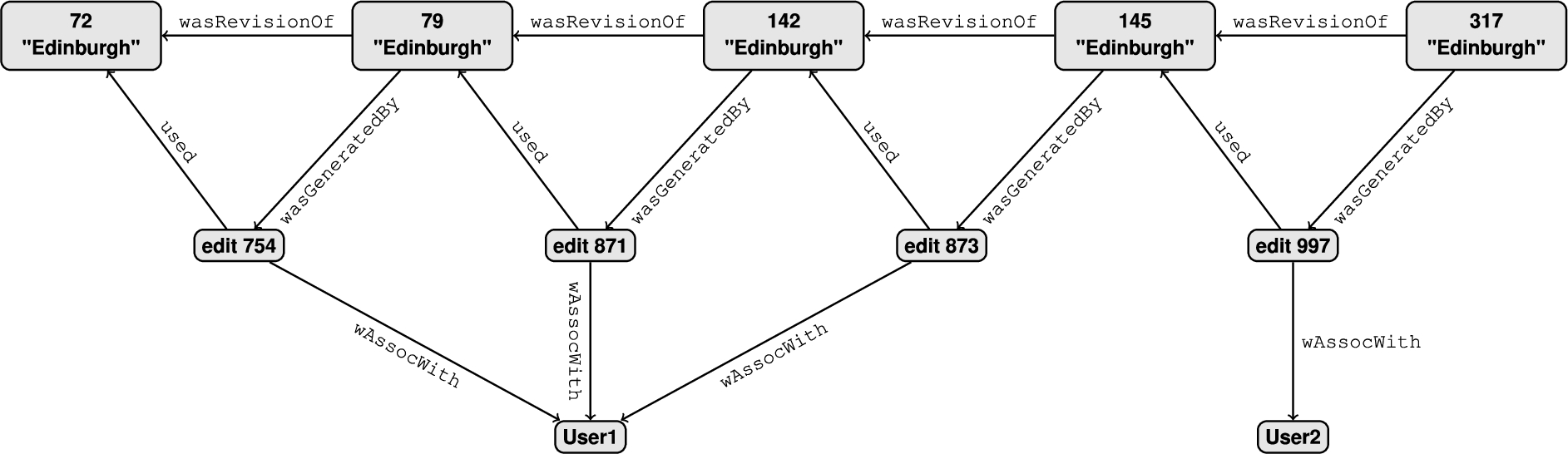
Looking for a recursive extension of SPARQL that can be easily implemented and adopted in practice, we turn to the option of adding a general recursion operator to SPARQL in a similar way to what has been done in SQL. To illustrate the need for such an operator we consider the case of tracking provenance of Wikipedia articles presented by Missier and Chen in [34]. They use the PROV standard [48] to store information about how a certain article was edited, whom was it edited by and what this change resulted in. Although they store the data in a graph database, all PROV data is easily representable as RDF using the PROV-O ontology [49]. The most common type of information in this RDF graph tells us when an article
A natural query to ask in this context is the history of revisions that were made by the same user: that is all pairs of articles
One possible reason why recursion was not previously considered as an integral operator of SPARQL could be the fact that in order to compute recursive queries we need to apply the query to the result of a previous computation. However, typical SPARQL queries do not have this capability as their inputs are RDF graphs but their outputs are mappings. This hinders the possibility of a fixed point recursion as the result of a SPARQL query cannot be subsequently queried. One can avoid this by using
In this paper we extend the recursion operator of [31] to function over a more widely used fragment of SPARQL and study how this operator can be implemented in an efficient and non-intrusive way on top of existing SPARQL engines. The main question we are trying to answer here is whether general purpose recursion is possible in SPARQL . We begin by showing what the general form of recursion looks like, what type of recursions we can support, the expressive power of the language, and how to evaluate it. We then argue that any implementation of this general form of recursion is unlikely to perform well on real world data, so we restrict it to the so called linear recursion, which is well known in the relational context [1,24]. We then argue that even this restricted class of queries can express most use cases for recursion found in practice. Next, we develop an elegant algorithm for evaluating this class of recursive queries and show how it can be implemented on top of an existing SPARQL system. For our implementation we use Apache Jena (version 3.7.0) framework [46] and we implement recursive queries as an add-on to the ARQ SPARQL query engine. We use Jena TDB (version 1), which allows us not to worry about queries whose intermediate results do not fit into main memory, thus resulting in a highly reliable system. Finally, we experimentally evaluate the performance of our implementation. For this, we begin by evaluating recursive queries in the context of smaller datasets such as YAGO and LMDB. We then compare our implementation to Jena and Virtuoso when it comes to property paths, using the GMark graph database benchmark [9], allowing us to gauge the effect of dataset size and query selectivity on execution times. In order to see how our solution scales, we also use the wikidata database and test the performance of recursive queries in this setting.11 We note that our main objective is not to find an optimal algorithms for evaluating recursion in SPARQL, but rather to show that recursion can be added in a non-intrusive way to the language, while still being capable of processing realistic workloads.
Related work As mentioned previously the most common type of recursion implemented in SPARQL systems are property paths. This is not surprising as property paths are a part of the latest language standard and there are now various systems supporting them either in a full capacity [25,52], or with some limitations that ensure they can be efficiently evaluated, most notable amongst them being Virtuoso [38]. The systems that support full property paths are capable of returning all pairs of nodes connected by a property path specified by the query, while Virtuoso needs a starting point in order to execute the query. From our analysis of expressive power we note that recursive queries we introduce are capable of expressing the transitive closure of any binary operator [31] and can thus be used to express property paths and any of their extensions [5,21,30,40,43]. Regarding attempts to implement a full-fledged recursion as a part of SPARQL, there have been none as far as we are aware. There were some attempts to use SQL recursion to implement property paths [51], or to allow recursion as a programming language construct [8,35], however none of them view recursion as a part of the language, but as an outside add-on. On the other hand, there is a wide body of work on implementing more powerful recursion in terms of datalog or other variants of logic programming (see e.g. [6,12,36]), but in this paper we are more interested in functionalities that can be added to SPARQL with little cost to systems in terms of extra software development.
Remark A preliminary version of this article was presented at the International Semantic Web Conference in 2015 [44]. The main contributions added to this manuscript not present in the conference version can be summarized as follows:
– Proofs of all the results. While the conference version of the paper provides only brief sketches of how the main results are proved, here we give complete proofs of all the stated theorems.
– Convergence conditions for recursion. We refine the analysis of when the recursion converges over RDF datasets, and fix a gap present in the conference version of the paper by introducing the notion of domain preserving queries.
– Analysis of expressive power. We analyse the expressive power of our language by comparing it to previous proposals, including Datalog [1], regular queries [43], and TriAL [32].
– Support for negation. We discuss possible extensions to the semantics in order to support negation inside recursive queries, or the BIND operator, which allows creating new values.
– Extensive experimental evaluation. The conference version of the paper only showcased the performance of our implementation over smaller datasets. Here we do a more robust analysis using the GMark graph database benchmark and the Wikidata dataset, in order to compare our approach to existing systems.
2.Preliminaries
Before defining our recursive operator we present the fragment of RDF and SPARQL we support. We first define what an RDF graph is, what operators we support and then we define their syntax and semantics.
RDF graphs and datasets. RDF graphs can be seen as edge-labeled graphs where edge labels can be nodes themselves, and an RDF dataset is a collection of RDF graphs. Formally, let I be an infinite set of IRIs and L an infinite set of Literals.22 An RDF triple is a tuple
An RDF graph is a finite set of RDF triples, and an RDF dataset is a set
Given two datasets D and
SPARQL syntax. We assume a countable infinite set V, called the set of variables, ∅ the unbound value and a set F, called the set of functions, that consists in functions of the form
The set of SPARQL queries is defined recursively as follows:
– An element of
– If
∗
∗
∗
∗
– If Q is a query and g is a variable or an IRI, then
– If Q is a query and
– If Q is a query and φ is a SPARQL buit-in condition (see below), then
– If Q is a query,
– A SPARQL built-in condition (or simply a filter-condition) is defined recursively as follows:
∗ An equality
∗ If ?x is a variable then
∗ A Boolean combination of filter-conditions (with operators ∧, ∨, and ¬) is a filter-condition.
Notably, we have chosen to rule out the EXISTS keyword. This is because of a disagreement in the semantics of this operator (see the discussion in [27]). However, once this agreement is settled, extending all of our results for queries with EXISTS will be a straightforward task.
Mappings and mappings sets. Since we have all the syntax of the language, we have to discuss the semantics, but before, we need to introduce the notion of mappings and some operators over sets of mappings. A SPARQL mapping is a partial function
Two mappings
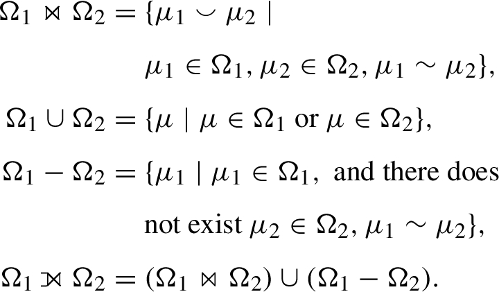
Let  are defined over sets of mappings as follows:
Given a query Q we write
SPARQL semantics. Let
– If t is a triple pattern, then
– If Q is
– If Q is
– If Q is
– If Q is
 .
.– If Q is
– If Q is
– If Q is
– If Q is
And finally, we define the semantics of built-in conditions. Let μ be a finite mapping from variables to elements in
– If φ is an equality
1.
2.
3.
– If φ is an expression of the form
– If φ is a Boolean combination of conditions using operators ∧, ∨ and ¬, then the truth value of
The CONSTRUCT operator The fragment of SPARQL graph patterns, as well as its generalisation to
The idea behind the
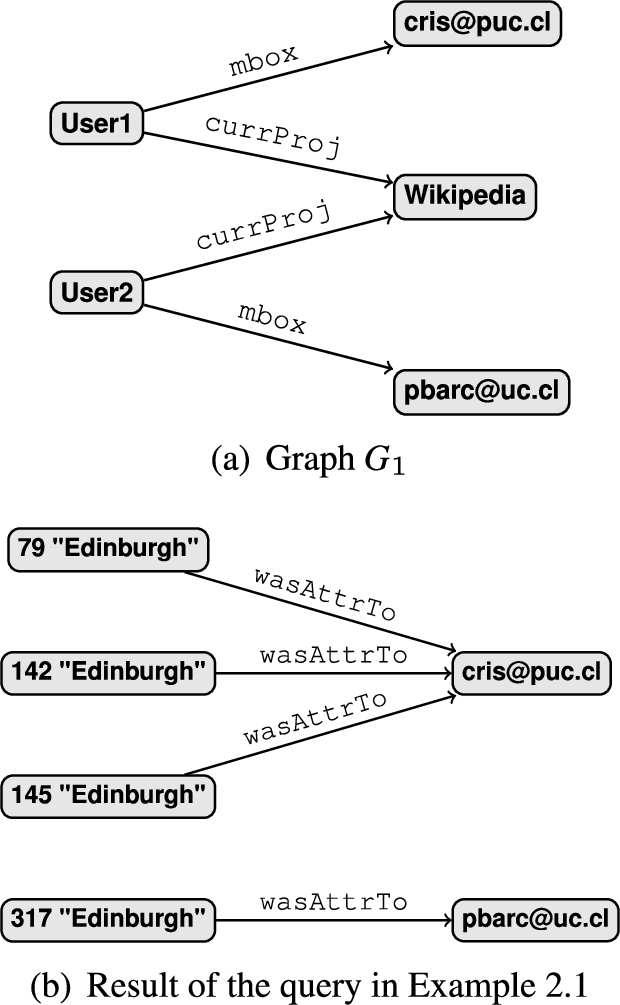
Example 2.1.
Let G be the graph in Fig. 1, and 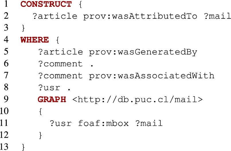
We call
For readability, we will use Q to refer to SPARQL queries using the SELECT form, and
3.Adding recursion to SPARQL
The most basic example of a recursive query in the RDF context is that of reachability: given a resource x, compute all the resources that are reachable from x via a path of arbitrary length. These type of queries, amongst others, motivated the inclusion of property paths into the SPARQL 1.1 standard [26].
However, as several authors subsequently pointed out, property paths fall short when trying to express queries that involve more complex ways of navigating RDF documents (cf. [5,17,18,40]) and as a result several extensions have been brought forward to combat this problem [2,13,21,30,32,40]. Almost all of these extensions are also based on the idea of computing paths between nodes in a recursive way, and thus share a number of practical problems with property paths. Most importantly, these queries need to be implemented using algorithms that are not standard in SPARQL databases, as they are based on automata-theoretic techniques, or clever ways of doing Breadth-first search over RDF documents.
3.1.A fixed point based recursive operator
We have decided to implement a different approach and define a more expressive recursive operator that allows us compute the fixed point of a wide range of SPARQL queries. This is based on the recursive operator that was added to SQL when considering similar challenges. We cannot define this type of operator for SPARQL
Example 3.1.
Recall graph G from Fig. 1. In the Introduction we made a case for the need of a query that could compute all pairs of articles
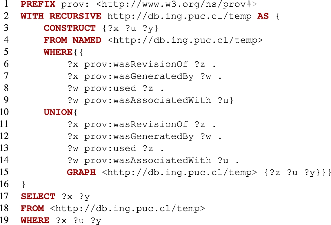
Fig. 3.
Example of a recursive query.
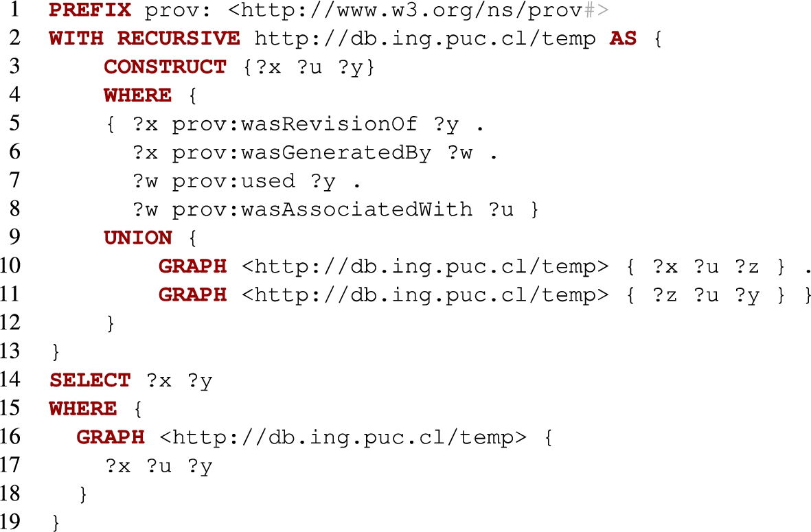
Let us explain how this query works. The second line specifies that a temporary graph named: http://db.ing.puc.cl/temp
will be constructed according to the query below which consists of a
Then comes the recursive part: if
We continue iterating until a fixed point is reached, and finally we obtain a graph that contains all the triples
As hinted in the example, the following is the syntax for recursive queries:
Definition 3.1
Definition 3.1(Syntax of recursive queries).
A recursive SPARQL query, or just recursive query, is either a SPARQL query or an expression of the form
Note that in this definition
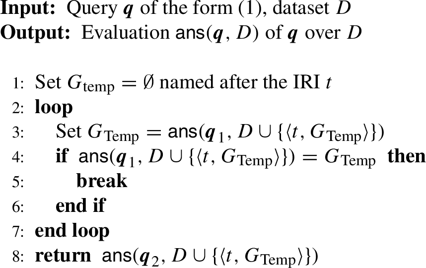
As usual with this type of queries, semantics is given via a fixed point iteration.
Definition 3.2
Definition 3.2(Semantics of recursive queries).
Let
In this definition,
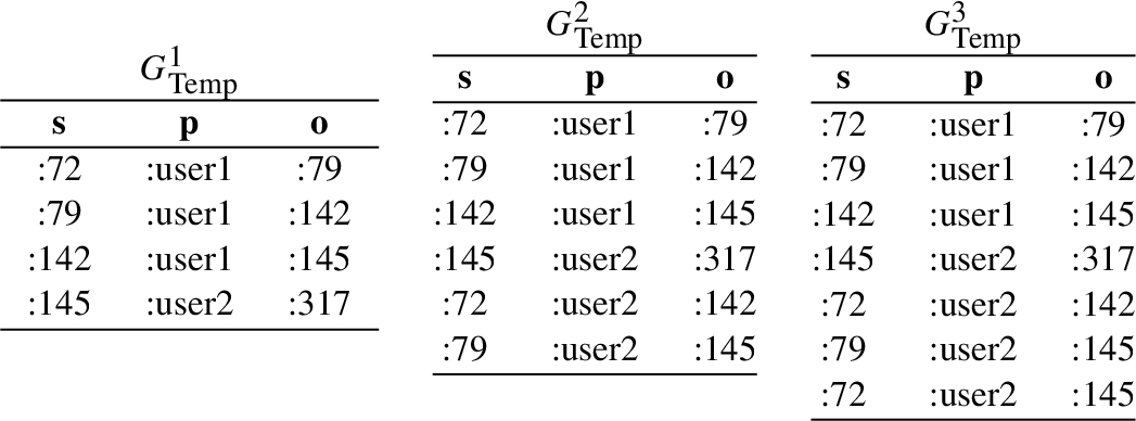
To clarify Definition 3.2, we show how the temporary graph <http://db.ing.puc.cl/temp> evolves during the execution of the query from Fig. 3, when evaluated the graph in Fig. 1. The different values of temporary graph are show in Fig. 4. Here we call
Obviously, the semantics of recursive queries only makes sense as long as the required fixed point exists. Unfortunately, we show in the following section that there are queries for which this operator indeed does not have a fixed point. Thus, we need to restrict the language that can be applied to such inner queries.55 We also discuss other possibilities to allow us using any operator we want.
3.2.Ensuring fixed point of queries
If we want to guarantee the termination of Algorithm 1, we need to impose two conditions. The first, and most widely studied, is that query
Monotonicity The most typical example of a problematic non-monotonic behaviour is when we use negation to alternate the presence of some triples in each iteration of the recursion, and therefore come up with recursive queries where the fixed point does not exists.
Example 3.2.
Consider the following query that contains a 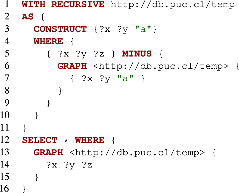
Also consider a instance for the default graph with only one triple:
:s :p "b"
In the first iteration, the graph <temp> would have the triple:
:s :p "a"
but in the next iteration the graph <temp> will be empty because of the
Similar examples can be obtained with other SPARQL operators that can simulate negation, such as
Preserving the domain The
Example 3.3.
Consider the following query that makes use of the 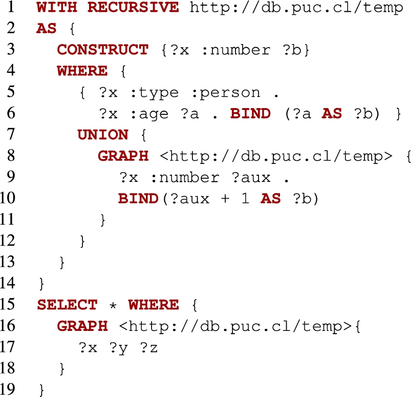
The base graph stores the age for all the people in the database. In each iteration, we will increase by one all the objects in our graph and then we will store triples with those new values. As we mentioned, in each iteration the query will try to insert new triples into the database, and will thus never terminate adding new triples into the dataset.
On the other hand, it is easy to verify that the query from Example 3.3 is monotone. By the Knaster–Tarski theorem [45], a monotone query always has a fixed point, however, such a fixed point need not be a finite dataset. Indeed, the fixed point for the query in Example 3.3 would have to contain triples linking each person in the original dataset with all the numbers larger than her or his initial age. This would make the fixed point infinite and thus not be a valid RDF graph.
One way to ensure that a fixed point of a monotone query is necessarily finite, is to make the underlying domain over which it operates finite. For instance, in Example 3.3, we are assuming that the domain over which queries operate is the set of all possible triple over
Besides the
Existence of a fixed point If we are working with queries that are both monotone and domain preserving, we can guarantee that the sequence
Proposition 3.1.
Let D be a dataset and
It is important to note that the query
Next, we study which SPARQL queries are both domain preserving and monotone, in order to restrict the recursion to such queries.
3.3.Fragments where the recursion converges
We know that monotonicity and domain preservation allows us to define a class of recursive queries which will always have a least fixed point. The question then is: how to define a fragment of SPARQL that is both monotonic and domain preserving?
First, how can we guarantee that queries are monotonic? An easy option here is to simply disallow all the operators which can simulate negation such as
Definition 3.3
Definition 3.3(positive SPARQL and rec-SPARQL).
A SPARQL query is positive if it does not use any of the following operators:
1. It does not use operators
2. Every construct
3. In every subquery
Given that positive SPARQL queries are both monotone and domain preserving, as an easy corollary of Proposition 3.1, we obtain the following:
Proposition 3.2.
If we have a recursive query
While positive queries do the trick, one might argue that they are quite restrictive. We can therefore wonder, whether it is possible to allow some form of negation, or the use of
In fact, literature has pointed out some more milder restrictions, that still do the trick. For instance, even though we disallow
The second, more expressive fragment to consider, loosens the restrictions we put on the use of negation. The idea is that bad behaviour of negation, such as the one shown in Example 3.2, only occurs when negation involves the same graph that is being constructed in the fixed point. Therefore, we will consider a fragment of rec-SPARQL queries which allow negation whenever it does not involve the graph being constructed in the recursive portion of the query.
Definition 3.4
Definition 3.4(Stratified positive rec-SPARQL).
Stratified positive rec-SPARQL extends the language of positive rec-SPARQL by allowing queries of the form (2) above in which
Essentially, with stratified positive rec-SPARQL we allow some degree of negation, but we need to make sure this negation does not involve the temporal graph under construction.
While stratified positive rec-SPARQL need not be monotone with respect to the domain of all possible RDF datasets, they are monotone in the context of the sequence
Proposition 3.3.
Let D be a dataset and
3.4.Expressive power
As a way to gauge the power of our language, we turn to the language datalog. Datalog (and ASP) has been used to pinpoint the expressive power of SPARQL (see e.g. [41]). For our case, it suffices to define positive Datalog, and Datalog with negation under stratified semantics.
A positive Datalog program Π consists of a finite set of rules of the form
Let P be an intensional predicate of a positive Datalog program Π and I a set of predicates. For
Datalog programs with negation extend positive datalog with rules of the form
For positive datalog programs Π with stratified negation, we can compute the answer
Since we are using Datalog to query RDF databases, we only focus on programs in which all extensional predicates are ternary predicates of the form
In order to study the expressive power of rec-SPARQL, we first compare positive c-queries and stratified positive c-queries with datalog. It follows from Polleres and Wallner [41] (see Table 1) that our fragment of positive c-queries can be translated into positive datalog, in the following sense: For each c-query
Proposition 3.4.
Let
Proof.
The idea is to proceed inductively. For a query
We note that the other direction is currently open: we do not know if every stratified positive datalog program can be translated into stratified positive rec-SPARQL. On the surface, and given the result that SPARQL can express all stratified positive datalog queries (see e.g. [31], it would appear that we can. However, rules in datalog programs may incur in all sort of simultaneous fixed points, as the dependency graph in programs need not be a tree. In standard datalog one can always flatten these simultaneous rules so that the resulting dependency graph is tree-shaped, but the only constructions we are aware of must incur in predicates with more than three positions, that we don’t currently know how to store in the graphs constructed by rec-SPARQL.
On the other hand, when datalog programs disallow all sort of simultaneous fixed points, a translation is surely possible.
Proposition 3.5.
Let Π be a positive (resp. stratified positive) datalog program, and assume that the only cicles on the dependency graph of Π are self loops. Then one can build a positive (resp. stratified positive) rec-SPARQL query
Proof.
That non-recursive datalog can be expressed as a c-query already follows from previous work [31]. By examining that proof, we get the following result: for each predicate S in a non-recursive program Π, if we assume that for each rule in Π of the form
Thus, all that remains to do is to lift this result for datalog programs when the only recursion is given by rules of the form
While this result may sound narrow, it already gives us a tool to compare again some other recursive languages proposed for graphs and RDF. For example, the language of regular queries [43] is a datalog program whose only cicles in its dependency graph are self loops, so we immedately have that rec-SPARQL can express any Regular Query. Another language with a similar recursion structure is TriAL [32], and we can also use that rec-SPARQL can express any TriAl query. On the other hand, it does not give us much in terms of more expressive languages such as [6], for which the comparison would require more work.
3.5.Complexity analysis
Since recursive queries can use either the
Proposition 3.6.
The problem SelectQueryAnswering is PSPACE-complete and ConstructQueryAnswering is NP-complete. The complexity of SelectQueryAnswering drops to
Proof.
It was proved in [31] that the problem ConstructQueryAnswering is NP-complete for non recursive c-queries, and Pérez et al. show in [39] that the problem SelectQueryAnswering if
To see that the upper bound is maintained, note that for each nested query, the temporal graph can have at most
Thus, at least from the point of view of computational complexity, our class of recursive queries are not more complex than standard select queries [39] or construct queries [31]. We also note that the complexity of similar recursive queries in most data models is typically complete for exponential time; what lowers our complexity is the fact that our temporary graphs are RDF graphs themselves, instead of arbitrary sets of mappings or relations.
For databases it is also common to study the data complexity of the query answering problem, that is, the same decision problems as above but considering the input query to be fixed. We denote this problems as SelectQueryAnswering
Proposition 3.7.
SelectQueryAnswering
Proof.
Following the same idea as in the proof of Proposition 3.6, we see that the number of iterations needed to construct the fixed point database is polynomial. But, if queries are fixed, the problem of evaluating
We prove the lower bound by a reduction from the path systems problem, which is a well known PTIME-complete problem (c.f. [47]). The problem is as follows. Consider a set of nodes V and a unary relation
For our reduction we construct a database instance and a (fixed) recursive query according to the instance of path systems such that the result of the query is empty if and only if
The database instance contains the information of which vertex is coloured, which vertex is part of the target relation T and the elements of the R relation:
– We define the function u which maps every vertex to a unique URI.
– For each element
– For each element
– For each element
Thus, the recursive query needs to compute all the coloured elements in order to check if the target relation is covered. This can be done in the following way: 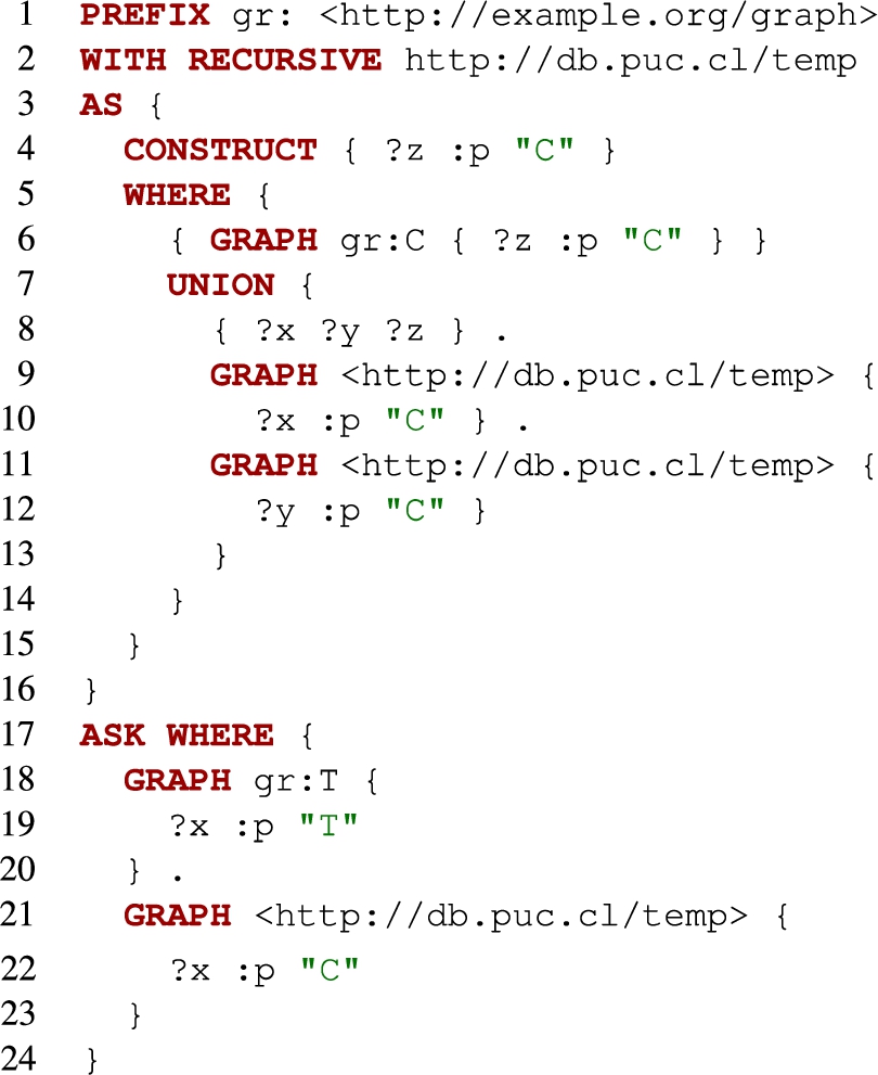
It is clear that the recursive part of the query is computing all the coloured nodes according to the R relation. Then in the ASK query, its result will be false iff none of the nodes in T are reachable. Note that this reduction can be immediately adapted to reflect hardness for queries using
From a practical point of view, and even if theoretically the problems have the same combined complexity as queries without recursion and are polynomial in data complexity, any implementation of the Algorithm 1 is likely to run excessively slow due to a high demand on computational resources (computing the temporary graph over and over again) and would thus not be useful in practice. For this reason, instead of implementing full-fledged recursion, we decided to support a fragment of recursive queries based on what is commonly known as linear recursive queries [1,24]. This restriction is common when implementing recursive operators in other database languages, most notably in SQL [42], but also in graph databases [18], as it offers a wider option of evaluation algorithms while maintaining the ability of expressing almost any recursive query that one could come up with in practice. For instance, as demonstrated in the following section, linear recursion captures all the examples we have considered thus far and it can also define any query that uses property paths. Furthermore, it can be implemented in an efficient way on top of any existing SPARQL engine using a simple and easy to understand algorithm. All of this is defined in the following section.
4.Realistic recursion in SPARQL
Having defined our recursive language, the next step is to outline a strategy for implementing it inside of a SPARQL system. In this section we show how this can be done by focusing on linear queries. While the use of linear queries is well established in the SQL context, here we show how this approach can be lifted to SPARQL. In doing so, we will argue that not only do linear queries allow for much faster evaluation algorithms than generic recursive queries, but they also contain many queries of practical interest. Additionally, we outline some alternatives of recursion which can support the use of negation or
4.1.Linear recursive queries
The concept of linear recursion is widely used as a restriction for fixed point operators in relational query languages, because it presents a good trade-off between the expressive power of recursive operators and their practical applicability.
Commonly defined for logic programs, the idea of linear queries is that each recursive construct can refer to the recursive graph or predicate being constructed only once. To achieve this, our queries are made from the union of a graph pattern that does not use the temporary IRI, denoted as
Notice that we enforce a syntactic separation between base and recursive query. This is done so that we can keep track of changes made in the temporary graph without the need of computing the difference of two graphs, as discussed in Section 4.2. This simple yet powerful syntax resembles the design choices taken in most SQL commercial systems supporting recursion,66 and is also present in graph databases [18].
To give an example of a linear query, we return to the query from Fig. 3. First, we notice that this query is not linear. Nevertheless, it can be restated as the query from Fig. 5 that uses one level of nesting (meaning that the query
Fig. 5.
Example of a linear recursion.
4.2.Algorithm for linear recursive queries
The main reason why linear queries are widely used in practice is the fact that they can be computed piece by piece, without ever invoking the complete database being constructed. More precisely, if a query
In other words, in order to compute the
Unfortunately, it is undecidable to check whether a given recursive query satisfies the property outlined above (under usual complexity-theoretic assumptions, see [23]), so this is why we must guarantee it with syntactic restrictions. We also note that most of the recursive extensions proposed for SPARLQ have the aforementioned property: from property paths [26] to nSPARQL [40], SPARQLeR [30], regular queries [43] or Trial [32], as well as our example.
As for the algorithm, we have decided to implement what is known as seminaive evaluation, although several other alternatives have been proposed for the evaluation of these types of queries (see [24] for a good survey). In order to describe our algorithm for evaluating a query of the shape (4), we abuse the notation and speak of
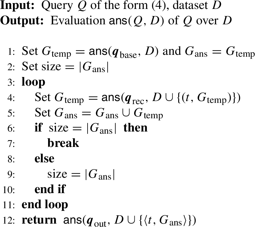
So what have we gained? By looking at Algorithm 2 one realizes that in each iteration we only evaluate the query over the union of the dataset and the intermediate graph
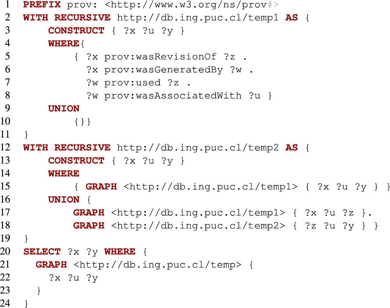
Expressive power of linear queries In Section 3.4 we show that all stratified positive recursive SPARQL queries can be defined in datalog, but have no matching result in the other direction. When it comes to linear queries, we can mirror the same result. The definition of linear datalog is quite straightforward: a datalog rule is linear if there is at most one atom in the body of the rule that is recursive with the head. For example, the rule
With this in mind, we can again show that every linear positive rec-SPARQL query can be transformed into linear positive datalog, and likewise for linear stratified positive rec-SPARQL and linear stratified datalog (note that the translation outlined in the proof of Proposition 3.4 preserves linearity). Unfortunately, for the other direction we have the same problem, as we are not sure whether our recursive languages can express every linear positive or stratified positive datalog program. Of course, we can also mirror Proposition 3.5 for linear queries. Thus, linear languages such as regular queries [43] or Trial [32] can be also translated into linear queries.
4.3.Supporting arbitrary queries in recursive clauses
Although we show in Section 3 that recursive queries which include some form of negation can be impossible to evaluate, there is no doubt that queries including negation are very useful in practice. In this section we briefly discuss how such queries can be mixed with linear recursion.
Limiting the recursion depth In practice it could happen that an user may not be interested in having all the answers for a recursive query. Instead, the user could prefer to have only the answers until a certain number of iterations are performed. We propose the following syntax for to restrict the depth of recursion to a user specified number k:
It is easy to see that this extension is useful for handling queries which include negation, or which create values by means of blanks or a
Other ways of supporting negation Limiting the number of iterations can also give us a way of allowing more complex c-queries inside the recursive part of recursive queries. This is not an elegant solution, but can be made to work: since the number of iterations is bounded, we don’t longer need queries to ensure that our graph has a fixed point operator.
We also mention that there are other, more elegant solutions, but we do not investigate them further as they drive us out of what can be implemented on top of SPARQL systems, and is out of the scope of this paper. For example, a possible solution to support
Studying these extensions to rec-SPARQL is an important topic for future work, and in particular the stable model semantics approach may require an interesting combination of techniques from both databases and logic programming.
5.Experimental evaluation
In this section we will discuss how our implementation performs in practice and how it compares to alternative approaches that are supported by existing RDF Systems. Though our implementation has more expressive power, we will see that the response time of our approach is similar to the response time of existing approaches, and also our implementation outperforms the existing solutions in several use cases.
Technical details Our implementation of linear recursive queries was carried out using the Apache Jena framework (version 3.7.0) [46] as an add-on to the ARQ SPARQL query engine. It allows the user to run queries either in main memory, or using disk storage when needed. The disk storage was managed by Jena TDB (version 1). As previously mentioned, since the query evaluation algorithms we develop make use of the same operations that already exist in current SPARQL engines, we can use those as a basis for the recursive extension to SPARQL we propose. In fact, as we show by implementing recursion on top of Jena, this capability can be added to an existing engine in an elegant and non-intrusive way.88
Datasets We test our implementation using four different datasets. The first one is Linked Movie Database (LMDB) [33], an RDF dataset containing information about movies and actors. The second dataset we use is a part of the YAGO ontology [50] and consists of all the facts that hold between instances. For the experiments the version from May 2018 was used. In order to test the performance of our implementation on synthetic data, we turn to the GMark benchmark [9], and generate data with different characteristics using this tool. Finally, we use the Wikidata “truthy” dump from 2018/11/15 containing over 3 billion triples, in order to test whether our implementation scales. All the datasets apart from Wikidata can be found at https://alanezz.github.io/RecSPARQL/.
Experiments The experiments we run are divided into four batches:
– Common use cases. In the first round of experiments we turn to YAGO and LMDB datasets, which allow defining recursive queries rather naturally. The main objective of these experiments is to show that our implementation can handle complex recursive patterns in reasonable time over real world datasets.
– Comparison with SPARQL engines. In order to compare with the recursive properties supported by SPARQL, we turn to the GMark [9] property path benchmark, and compare our implementation with pache Jena and Openlink Virtuoso, two popular SPARQL systems.
– Performance over large datasets. To verify whether our solution scales, we run a sequence of recursive queries over the Wikidata dataset containing over 3 billon triples, and compare our response times with the ones provided by the Wikidata endpoint.
– Limiting recursion depth. Finally, we test the solution proposed in Section 4.3, which stops the recursive iteration after a predetermined number of steps. Here we show that this approach is not only useful fro dealing with recursion, but also when evaluating repeated joins.
The experiments involving smaller datasets (LMDB, YAGO, and GMark) were run on a MacBook Pro with an Intel Core i5 2.6 GHz processor and 8 GB of main memory. To handle the size of Wikidata, we used a server Devuan GNU/Linux 3 (beowulf) with an Intel Xeon Silver 4110 CPU @ 2.10 GHz processor and 120 GB of memory.
Next, we elaborate on each batch of experiments, as specified above.
5.1.Evaluating real use cases
The first thing we do is to test our implementation against realistic use cases. As we have mentioned, we do not aim to obtain the fastest possible algorithms for these particular use cases (this is out of the scope of this paper), but rather aim for an implementation whose execution times are reasonable. For this, we took the LMDB and the YAGO datasets, and built a series of queries asking for relationships between entities. Since YAGO also contains information about movies, we have the advantage of being able to test the same queries over different datasets (their ontology differs). The specifications for each database can be found in the Table 1. Note that the size is the one used by Jena TDB to store the datasets.
Table 1
Specifications for the LMDB and Yago datasets
| Graph | Number of triples | Size |
| LMDB | 6147996 | 1.09 Gb |
| Yago | 6215350 | 1.54 Gb |
To the best of our knowledge, it is not possible to compare the full scope of our approach against other implementations. While it is true that our formalism is similar to the recursive part of SQL, all of the RDF systems that we checked were either running RDF natively, or running on top of a relational DBMS that did not support the recursion with common table expressions functionality, that is part of the SQL standard. OpenLink Virtuoso does have a transitive closure operator that can be used with its SQL engine, but this operator is quite limited in the sense that it can only compute transitivity when starting in a given IRI. Our queries were more general than this, and thus we could not compare them directly. For this reason, in this set of experiments we will only discuss about the practical applicability of the results.
Our round of experiments consists of three movie-related queries, which will be executed both on LMDB and YAGO, and two additional queries that are only run in YAGO, because LMDB does not contain this information. All of these queries are similar to that of Example 3.1 (precise queries are given in the Appendix). The queries executed in both datasets are the following:
– QA: the first query returns all the actors in the database that have a finite Bacon number,99 meaning that they co-starred in the same movie with Kevin Bacon, or another actor with a finite Bacon number. A similar notion, well known in mathematics, is that of an Erdős number.
– QB: the second query returns all actors with a finite Bacon number such that all the collaborations were done in movies with the same director.
– QC: the third query tests if an actor is connected to Kevin Bacon through movies where the director is also an actor (not necessarily in the same movie).
The queries executed only in the YAGO dataset where the following:
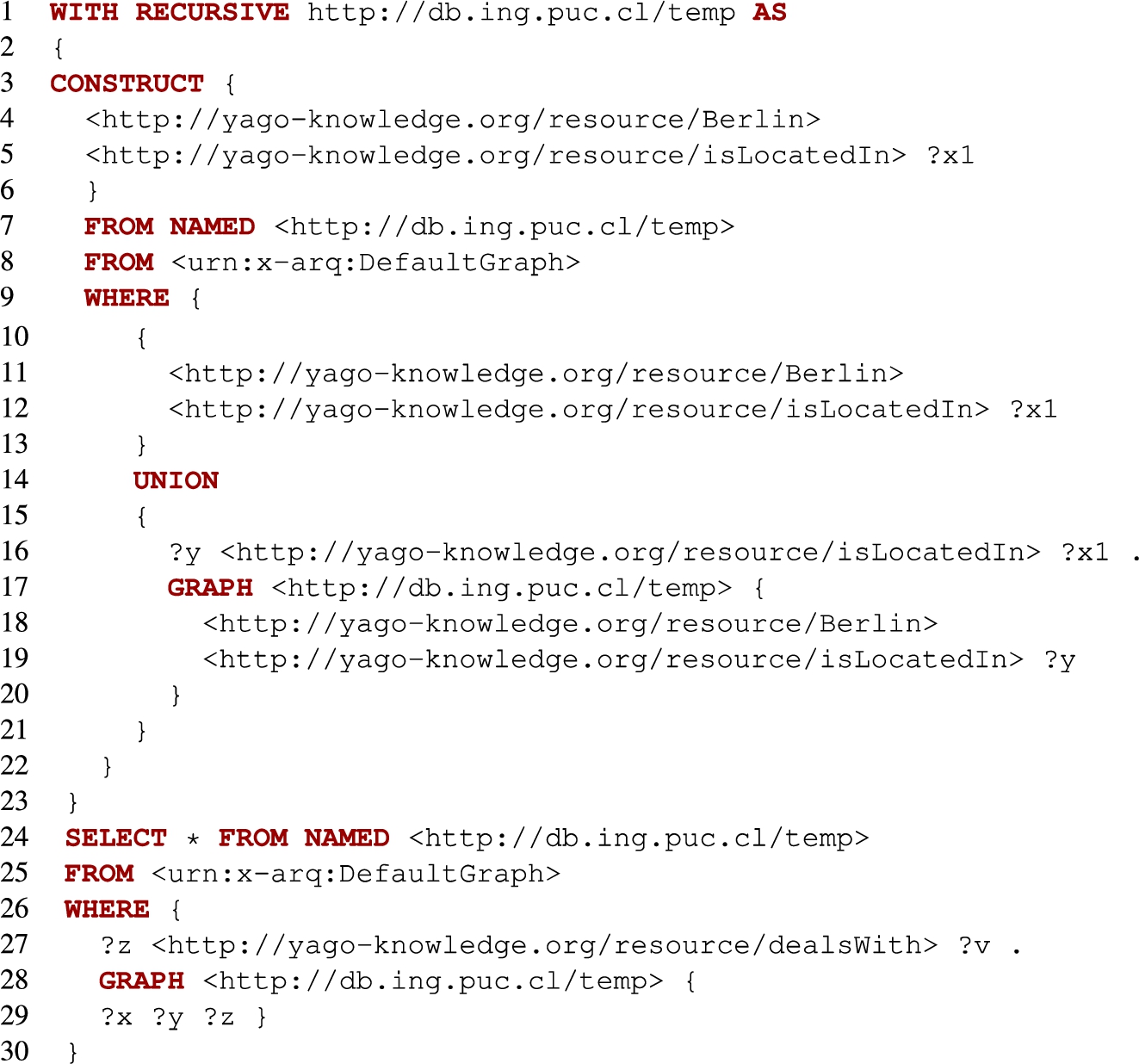
– QD: the fourth query answers with the places where the city Berlin is located in from a transitive point of view, starting from Germany, then Europe and so forth.
– QE: the fifth query returns all the people who are transitively related to someone, through the isMarriedTo relation, living in the United States or some place located within the United States.
Note that QA, QD and QE are also expressible as property paths. To fully test recursive capabilities of our implementation we use another two queries, QB and QC, that apply various tests along the paths computing the Bacon number. Recall that the structure of queries QB and QC is similar to the query from Example 3.1 and cannot be expressed in SPARQL 1.1 either.
Fig. 6.
Running times and the number of output tuples for the three datasets.
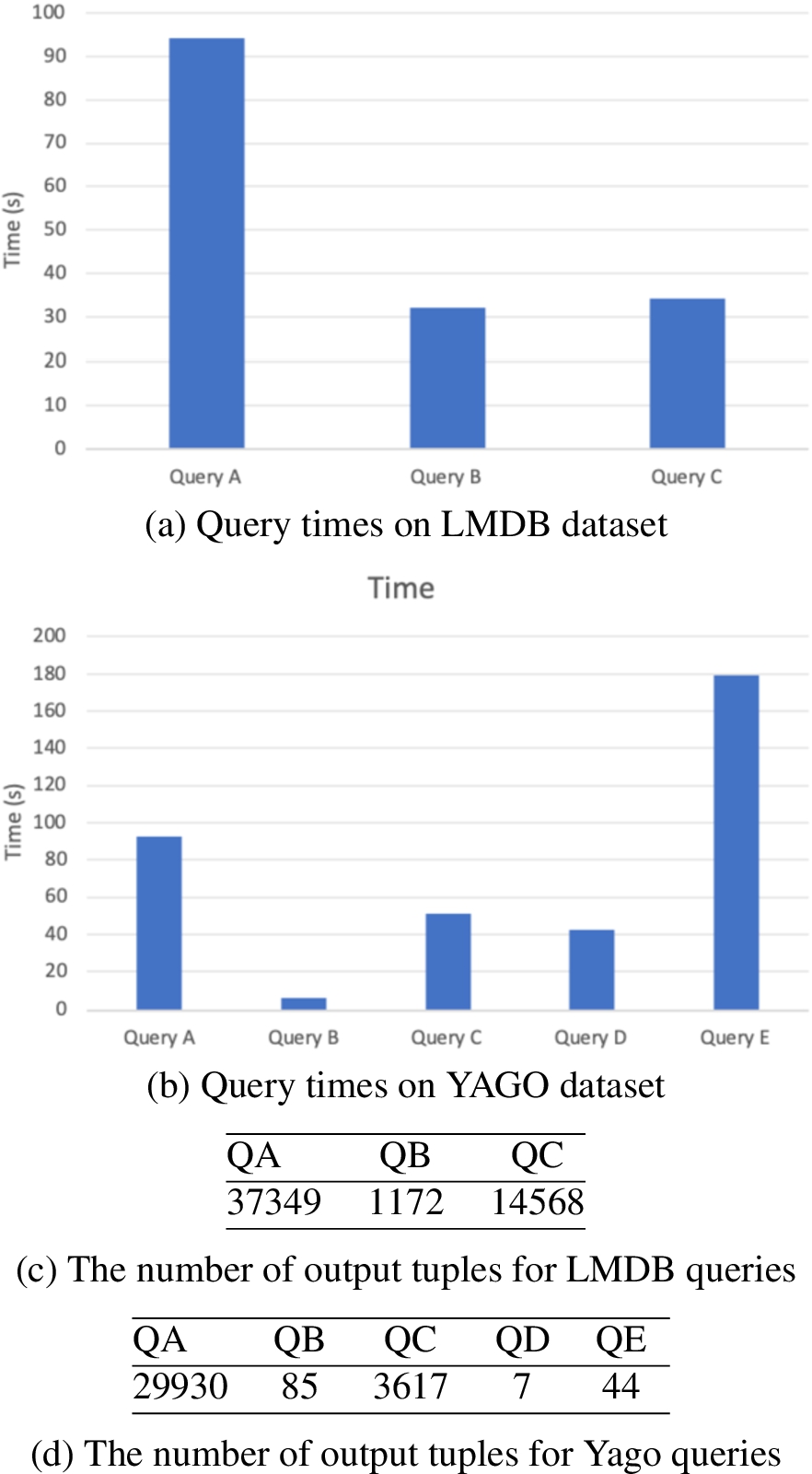
The results of the evaluation can be found in Figs 6(a) and 6(b). As we can see the running times, although high, are reasonable considering the size of the datasets and the number of output tuples (Figs 6(c) and 6(d)). The query QE is the only query with a small size in its output and a high time of execution. This fact can be explained because the query is a combination of 2 property paths that required to instantiate 2 recursive graphs before computing the answer.
5.2.Comparison with property paths using the GMark benchmark
As mentioned previously, since to the best of our knowledge no SPARQL engine implements general recursive queries, we cannot really compare the performance of our implementation with the existing systems. The only form of recursion mandated by the latest language standard are property paths, so in this section we show the results of comparing the execution of property paths queries in our implementation using our recursive language against the implementation of property paths in popular systems.
We used the GMark benchmark [9] to measure the running time of property paths queries using Recursive SPARQL, and to compare such times with respect to Apache Jena and Openlink Virtuoso.
The GMark benchmark allows generating queries and datasets to test property paths, and one of its advantages is that the size of the datasets and the patterns described by the queries are parametrized by the user. Using the benchmark we generated three different graphs of increasing size, named
Table 2
Specifications for the graphs generated by GMark
| Graph | Number of triples | Size |
| 220564 | 271 mb | |
| 447851 | 535 mb | |
| 671712 | 605 mb |
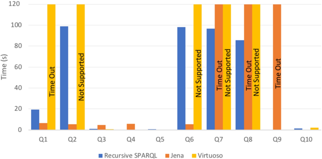
Fig. 7.
Times for
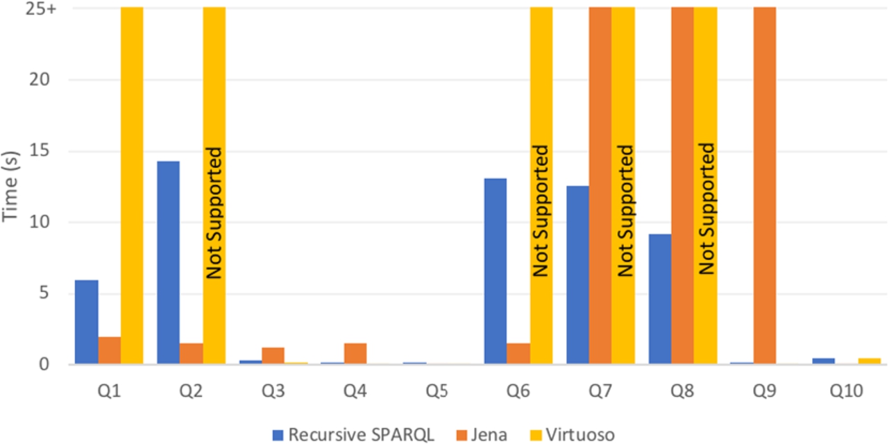
Fig. 8.
Times for
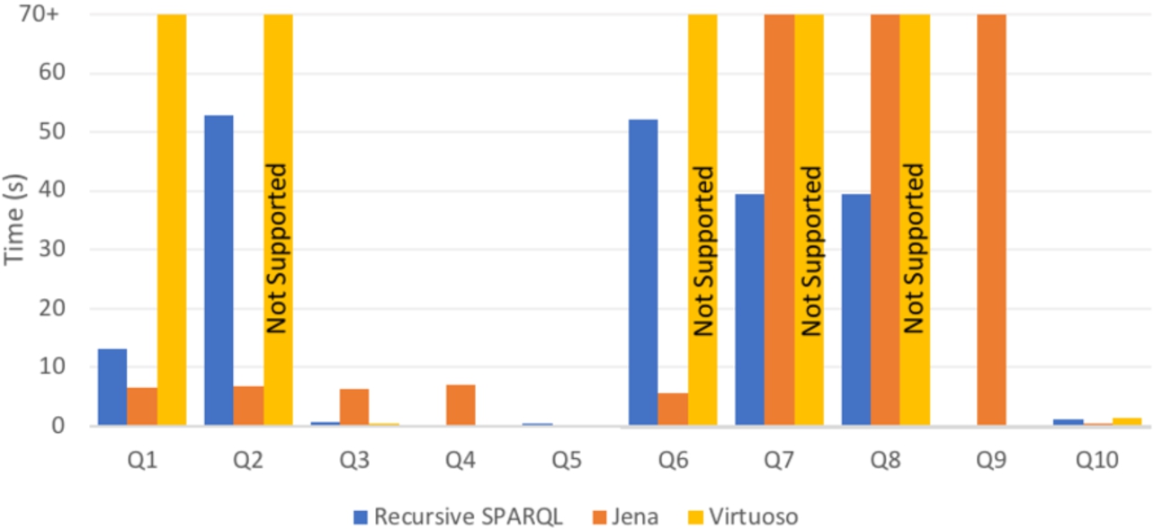
Fig. 9.
Times for
Note first that every property path query is easily expressible using linear recursion. With this observation in mind we must also remark that we are comparing the performance of our more general recursive engine with property paths, which are a much less expressive language. For this reason highly efficient systems like Virtuoso should run property paths queries faster: they do not need to worry about being able to compute more recursive queries. Of course, it would also be interesting to compare our engine with specific ad-hoc techniques for computing property paths.
Table 3
Number of outputs for the GMark queries over the graph
| System | Q1 | Q2 | Q3 | Q4 | Q5 | Q6 | Q7 | Q8 | Q9 | Q10 |
| RecSPARQL | 24723 | 3964 | 1455 | 9 | 169 | 3964 | 2604 | 126 | 2 | 906 |
| Jena | 103814 | 90398 | 89128 | 198 | 802 | 90398 | 10838 | 94638 | 89523 | 5373 |
| Virtuoso | 1849915 | – | 2267 | 198 | 804 | – | – | – | 454 | 6345 |
Comparison with Virtuoso Virtuoso cannot run queries 2, 6, 7 and 8, because the SPARQL engine requires an starting point for property paths queries, which was not possible to give for such queries. We can see that Virtuoso outperforms Jena and the Recursive implementation in almost all the queries that they can run, except for Query 1, where the running time goes beyond 25 seconds. As we will discuss later, this can be explained because of the semantic they use to evaluate property paths, which makes Virtuoso to have many duplicated answers. For the remaining queries, we can see that the execution time is almost equals.
Comparison with Jena Apache Jena can also answer all queries. However, our recursive implementation is only clearly outperformed in Query 2 and Query 6. This is mainly because those queries have patterns of the form:
?x <:p1|:p2>* ?z
and our system is not optimized for working with unions of predicates. Remarkably, and even though all of the generated queries are relatively simple, our implementation reports a faster running time in half of the queries we test. Note that Q7, Q8 and Q9 have an answer time considerably worse in Jena than in our recursive implementation, where the time goes beyond the 25 seconds. We can only speculate that this is because the property paths has many paths of short length and because Apache Jena cannot manage properly the queries with two or more star triple patterns.
When we increase the size of the graph, the results have the same behaviour. It is also more evident which queries are easier and harder to evaluate for the existing systems. The result for the increased size of the graph can be found in the Figs 8 and 9.
Number of outputs As we said before, one interesting thing that we note from the previous experiments is the time that Virtuoso took to answer the query Q1 in the three dataset. We suspect that this could occur because Virtuoso generates many duplicate results, thus the output should be higher with respect to rec-SPARQL and Jena. We count the number of outputs for the queries ran over the first graph. The results can be seen in Table 3.
The first thing to note is that we avoid duplicate answers in our language, mainly because of the UNION operator used in lineal recursion, which deletes the duplicates answers. Also we do not consider paths of length 0, because those results do not give us any relevant information about the answer. Then we can see that Apache Jena has always more results than us, this is mainly because they consider paths of length 0. We did not rewrite the queries because we wanted keep them as close as possible to the benchmark. In Virtuoso one needs a starting point for property path queries, so this system does not consider paths of length 0 and for that reason in some queries they have less outputs than Apache Jena. However, in most of the queries they give more results than Apache Jena and RecSPARQL, because they produce many duplicate answers and thus, the answer time becomes considerably worse. This happen mainly in the first query, which is the simplest one. The same effect happen for the 2 bigger graphs. The number of outputs for the bigger graphs can be found in the Appendix (Tables 5 and 6).
5.3.Tests over large datasets
We wanted to know how our recursive operator works when the queries are executed over large datasets. Thus, we decided to try our implementation with queries over the graph of Wikidata, so we load the “truthy” dump from 2018/11/15. This dump contains 3,303,288,386 triples. For this set of experiments we use a server Devuan GNU/Linux 3 (beowulf) with an Intel Xeon Silver 4110 CPU @ 2.10 GHz processor and 120 GB of memory.
We create property paths queries based on (1) the example queries showed at the Wikidata Endpoint and (2) the LMDB queries from Section 5.1. The queries are the following:
– Q1: Sub-properties of property P276.
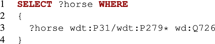
– Q2: All the instances of horse or a subclass of horse.
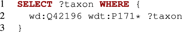
– Q3: Parent taxon of the Blue Whale.
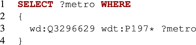
– Q4: Metro stations reachable from Palermo Station in Metro de Buenos Aires.
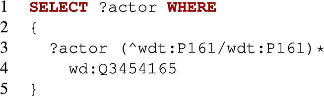
– Q5: Actors with finite Bacon number:
Queries Q1, and Q4 are simple star * queries, while Q3 is a star query where in each iteration only one triple is added to the recursive graph. Q2 is a query of the form (wdt:p1/wdt:p2*), while Q5 combines two properties within a star.
We rewrote the property paths as WITHRECURSIVE queries and we ran them on our server setup. We display the results in Table 4. As a reference, we also put the time that the queries took at the Wikidata endpoint https://query.wikidata.org/. We note that this is not an exact comparison as the endpoint dataset might slightly differ from the one we use, and the server running the endpoint is likely different from ours. The values are expressed in seconds.
Table 4
Time in seconds taken by the queries over the Wikidata Graph
| Query | RecSPARQL | Endpoint |
| Q1 | 2.23 | 0.28 |
| Q2 | 2.45 | 1.02 |
| Q3 | 2.15 | 0.56 |
| Q4 | 2.11 | 0.73 |
| Q5 | 101.60 | Timeout |
As we see, the trend shown with the previous experiments is repeated again with a large dataset: Recursive SPARQL is competitive against existing solutions. Since the dataset of Wikidata is larger than previous datasets and our solution implies to do several joins, we expected easier queries to have better running times in the endpoint than in our implementation. However, the running times our solution displays are still competitive. Finally, we remark the result for Q5, where our implementation could answer the query in a reasonable time, and the endpoint times out.
5.4.Limiting the number of iterations
In Section 4.3 we presented a way of limiting the depth of the recursion. We argue that this functionality should find good practical uses, because users are often interested in running recursive queries only for a predefined number of iterations. For instance, very long paths between nodes are seldom of interest and in a wast majority of use cases we will be interested in using property paths only up to depth four or five.
It is straightforward to see that every query defined using recursion with predefined number of iterations can be rewritten in SPARQL by explicitly specifying each step of the recursion and joining them using the concatenation operator. The question then is, why is specifying the recursion depth beneficial?
One apparent reason is that it makes queries much easier to write and understand (as a reference we include the rewritings of the query QA, QB and QC from Section 5.1 using only SPARQL operators in the online Appendix). The second reason we would like to argue for is that, when implemented using Algorithm 2, recursive queries with a predetermined number of steps result in faster query evaluation times than evaluating an equivalent query with lots of joins. The intuitive reason behind this is that computing
We substantiate this claim by running two rounds of experiments on LMDB and YAGO datasets, using queries QA, QB and QC from Section 5.1 and running them for an increasing number of steps. We evaluate each of the queries using Algorithm 2 and run it for a fixed number of steps until the algorithm saturates. Then we use a SPARQL rewriting of a recursive query where the depth of recursion is fixed and evaluate it in Jena and Virtuoso.
Fig. 10.
Limiting the number of iterations for the evaluation of
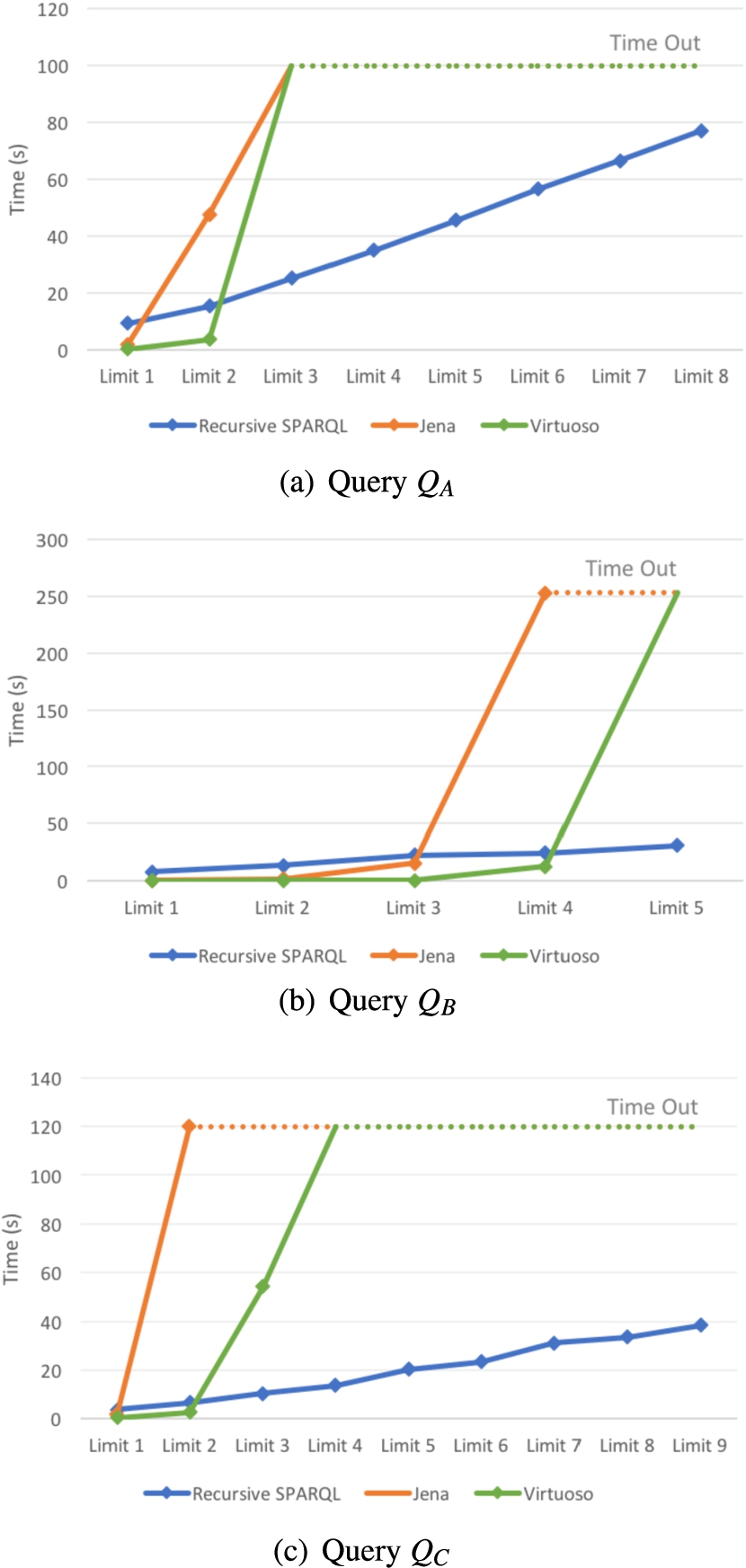
Fig. 11.
Limiting the number of iterations for the evaluation of
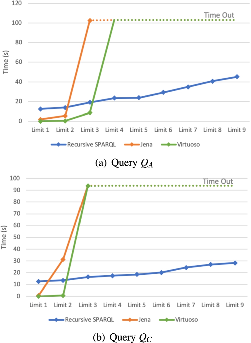
Figure 10 shows the results over LMDB and Fig. 11 shows the results over YAGO. The time out here is again set to two minutes. As we can see, the initial cost is much higher if we are using recursive queries, however as the number of steps increases we can see that they show much better performance and in fact, the queries that use only SPARQL operators time out after a small number of iterations. Note that we did not run the second query over the YAGO dataset, because it ends in two iterations, and it would not show any trend. We also did not run queries QD and QE. Query QD was timing out also after two iterations on Jena and Virtuoso, and query QE is composed of two property paths, so there is no straightforward way to transform it in a query with unions.
6.Conclusions and looking ahead
As illustrated by several use cases, there is a need for recursive functionalities in SPARQL that go beyond the scope of property paths. To tackle this issue we propose a recursive operator to be added to the language and show how it can be implemented efficiently on top of existing SPARQL systems. We concentrated on linear recursive queries which have been well established in SQL practice and cover the majority of interesting use cases and show how to implement them as an extension to Jena framework. We then test on real world datasets to show that, although very expressive, these queries run in reasonable time even on a machine with limited computational resources. Additionally, we also include the variant of the recursion operator that runs the recursive query for a limited number of steps and show that the proposed implementation outperforms equivalent queries specified using only SPARQL 1.1 operators.
Given that recursion can express many requirements outside of the scope of SPARQL 1.1, coupled with the fact that implementing the recursive operator on top of existing SPARQL engines does not require to change their core functionalities, allows us to make a strong case for including recursion in the future iterations of the SPARQL standard. Of course, such an expressive recursive operator is not expected to beat specific algorithms for smaller fragments such as property paths. But nothing prevents the language to have both a syntax for property paths and also for recursive queries, with different algorithms for each operator.
There are several other areas where a recursive operator should bring immediate impact. To begin with, it has been shown that a wide fragment of recursive SHACL constraints can be compiled into recursive SPARQL queries [19], and a similar result should hold for ShEx constraints [15]. Another interesting direction is managing ontological knowledge. Indeed, it was shown that even a mild form of recursion is sufficient to capture RDFS entailment regimes [40] or OWL2 QL entailment [14], and it stands open to which extent can rec-SPARQL help us capture more complex ontologies, and evaluate them efficiently. Furthermore, rec-SPARQL may also be used for other applications such as Graph Analytics or Business Intelligence.
Looking ahead, there are several directions we plan to explore. We believe that the connection between recursive SPARQL and RDF shape schemas should be pursued further, and so is the connection with more powerful languages for ontologies. There is also the subject of finding the best semantics for recursive SPARQL queries involving non-monotonic definitions. Stable model semantics may or may not be the best option, and even if it is, it would be interesting to see if one can obtain a good implementation by leveraging techniques developed for logic programming, or provide tools to compile recursive SPARQL queries into a logic program. Regarding blanks and numbers, perhaps one can also find a reasonable fragment, or a reasonable extension to the semantics of recursive queries, that can deal with numbers and blanks, but that can still be evaluated under the good properties we have showcase for linear recursion.
Finally, there is also the question of what is the best way of implementing these languages. In this paper we have explored the idea of implementing recursive SPARQL on top of a database system, as is done in SQL. As we discussed, this approach has numerous advantages, and it shows that recursion can be added to SPARQL with little overhead for the companies providing SPARQL processors. However, another option would be to use more powerful engines capable of running full datalog or similarly powerful languages (see e.g. [36] or [12]), which may provide better running times than our on-top-of-system implementation, and should be able to run non-linear queries. This is another source of questions that would require closer work between database and logic programming communities.
Notes
1 The implementation, test data, and complete formulation of all the queries can be found at https://alanezz.github.io/RecSPARQL/.
2 For clarity of presentation we do not include blank nodes in our definitions.
3 For brevity we leave out FROM named constructs, and we leave the study of blanks in templates as future work.
4 For readability we assume that t is not a named graph in D. If this is not the case then the pseudocode needs to be modified to meet the definition above.
5 It should be noted that the recursive SQL operator has the same problem, and indeed the SQL standard restricts which SQL features can appear inside a recursive operator.
6 In SQL one cannot execute a recursive query which is not divided by
7 Interestingly, one can show that in this case the nesting in this query can be avoided, and indeed an equivalent non-nested recursive query is given in the Appendix.
8 The implementation we use is available at https://alanezz.github.io/RecSPARQL/.
Acknowledgements
This work was supported by the Millennium Institute for Foundational Research on Data (IMFD) and by CONICYT-PCHA Doctorado Nacional 2017-21171731.
Appendices
Appendix
Here we present some of the queries that we ran throughout this work. Note that here we declare the queries using the clauses FROM and FROM NAMED. This is because some systems need the declaration of the graphs that are used in GRAPH clauses.
Queries from Section 5.1
The query
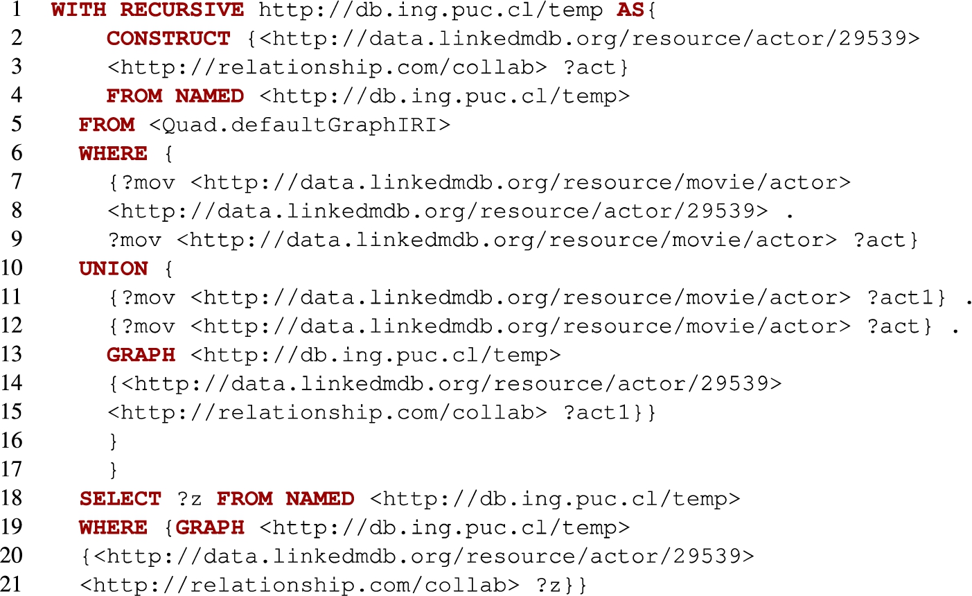
The following is the formulation of the query

The following is the formulation of the query
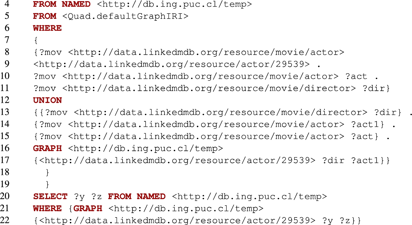
The following is the formulation of the query
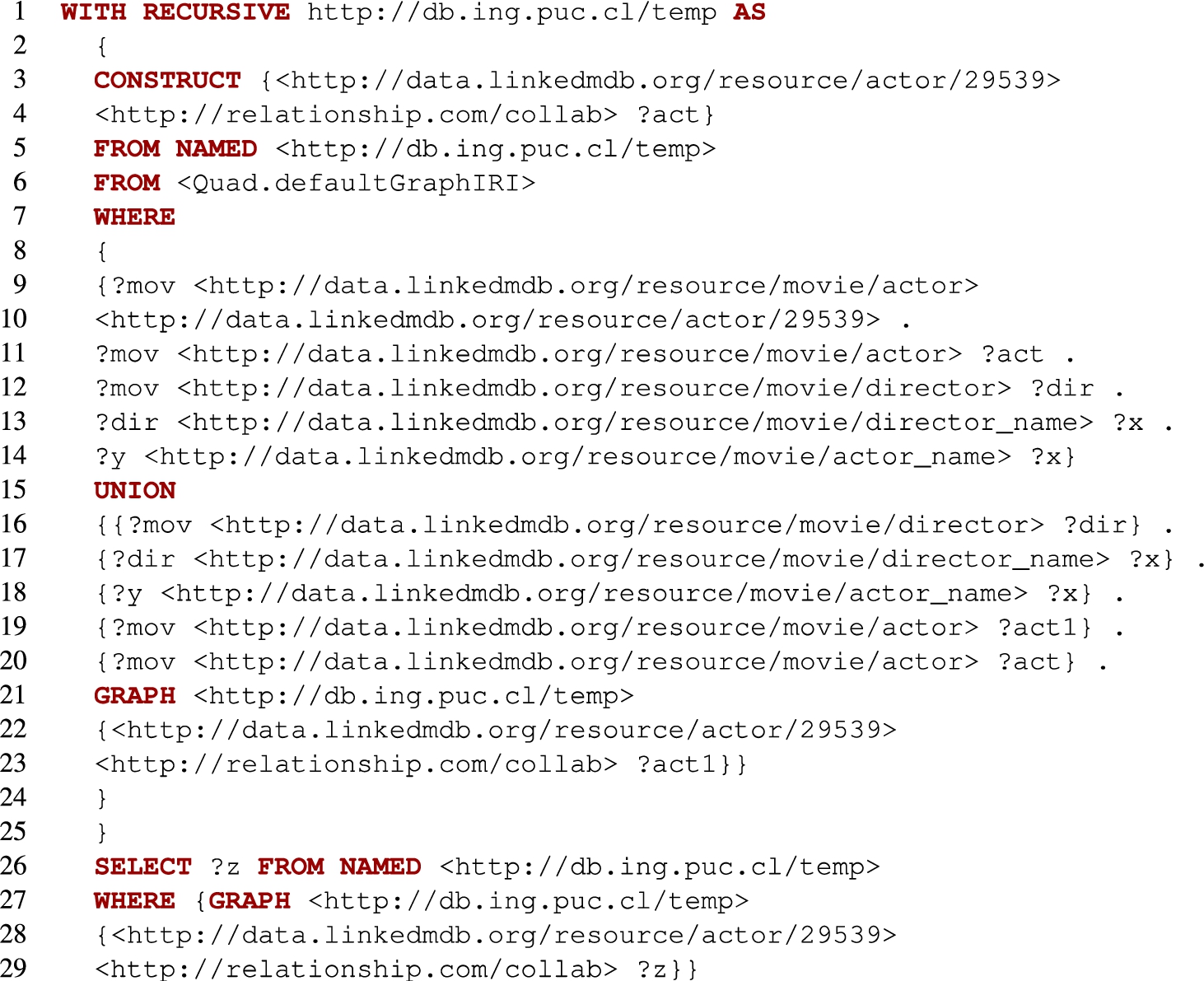
The following is the formulation of the query 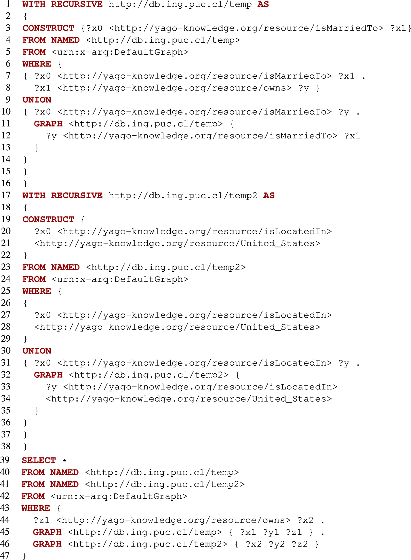
Queries from Section 5.2
The following are the queries generated by the GMark benchmark:
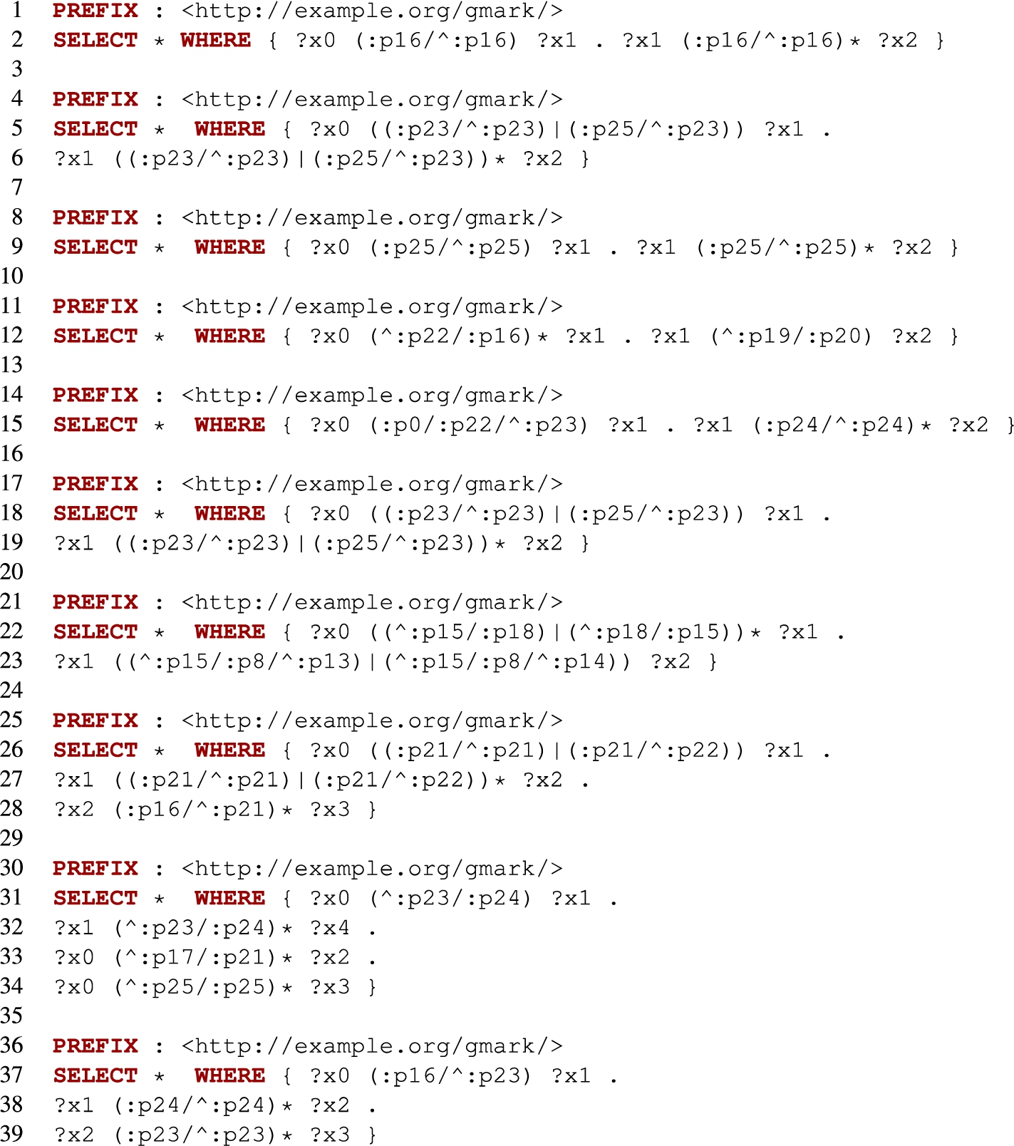
The same queries written in Recursive SPARQL can be found at https://alanezz.github.io/RecSPARQL.
Queries from Section 4.3
The following is SPARQL rewriting of the query Q1 computing Bacon number of length at most 5:
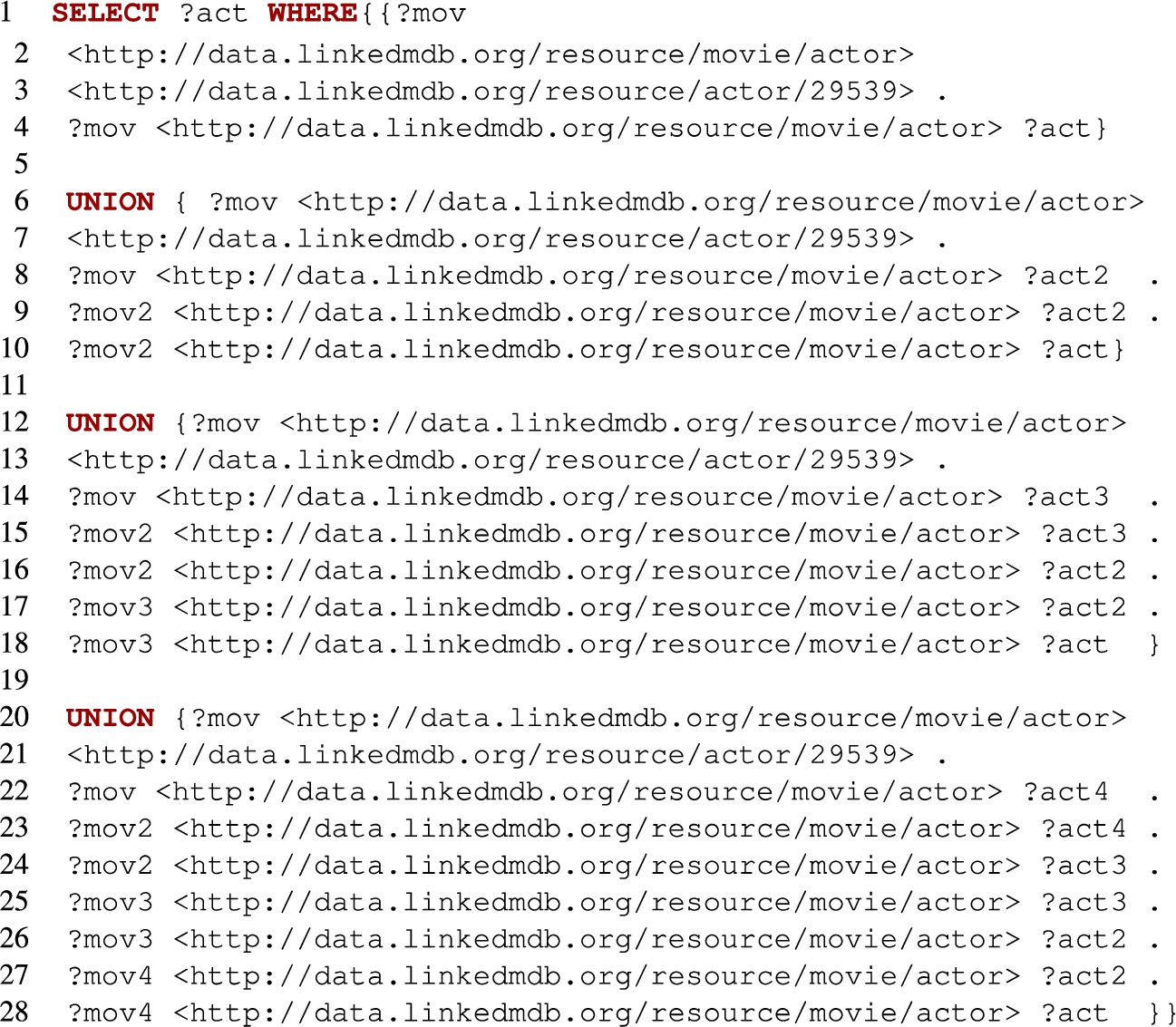
Other rewritings are similar and can be found at https://alanezz.github.io/RecSPARQL.
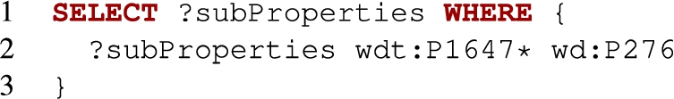
Queries over the wikidata endpoint
– Q1: Sub-properties of property P276:
– Q2: Horse lineages:
– Q3: Parent taxon of the Blue Whale:
– Q4: Metro stations reachable from Palermo Station in Metro de Buenos Aires:
– Q5: Actors with finite Bacon number:
Number of outputs for the bigger graphs in GMark
The number of outputs for the bigger graphs can be found in Tables 5 and 6.
Table 5
Number of outputs for the GMark queries over the graph
| System | Q1 | Q2 | Q3 | Q4 | Q5 | Q6 | Q7 | Q8 | Q9 | Q10 |
| RecSPARQL | 50190 | 8153 | 3188 | 7 | 345 | 8153 | 6116 | 308 | 4 | 2134 |
| Jena | 208437 | 181043 | 178465 | 409 | 1547 | 181043 | 16730 | 189628 | 179168 | 11022 |
| Virtuoso | 3624482 | – | 5256 | 409 | 1561 | – | – | – | 968 | 13002 |
Table 6
Number of outputs for the GMark queries over the graph
| System | Q1 | Q2 | Q3 | Q4 | Q5 | Q6 | Q7 | Q8 | Q9 | Q10 |
| RecSPARQL | 74967 | 12015 | 4719 | 17 | 533 | 12015 | 16040 | 487 | 4 | 2942 |
| Jena | 311559 | 270506 | 266777 | 766 | 2674 | 270506 | – | – | – | 15951 |
| Virtuoso | – | – | 7743 | 766 | 2716 | – | – | – | 1384 | 18726 |
References
[1] | S. Abiteboul, R. Hull and V. Vianu, Foundations of Databases, Addison-Wesley, (1995) . |
[2] | F. Alkhateeb, J.-F. Baget and J. Euzenat, Extending SPARQL with regular expression patterns (for querying RDF), J. Web Sem. 7: (2) ((2009) ), 57–73. doi:10.1016/j.websem.2009.02.002. |
[3] | R. Angles, M. Arenas, P. Barceló, A. Hogan, J. Reutter and D. Vrgoč, Foundations of modern query languages for graph databases, ACM Computing Surveys (CSUR) 50: (5) ((2017) ), 1–40. doi:10.1145/3104031. |
[4] | R. Angles and C. Gutierrez, The multiset semantics of SPARQL patterns, in: International Semantic Web Conference, Springer, (2016) , pp. 20–36. doi:10.1007/978-3-319-46523-4_2. |
[5] | K. Anyanwu and A.P. Sheth, ρ-Queries: Enabling querying for semantic associations on the semantic web, in: 12th International World Wide Web Conference (WWW), (2003) . |
[6] | M. Arenas, G. Gottlob and A. Pieris, Expressive languages for querying the semantic web, in: Proceedings of the 33rd ACM SIGMOD-SIGACT-SIGART Symposium on Principles of Database Systems, (2014) , pp. 14–26. doi:10.1145/2594538.2594555. |
[7] | M. Arenas, C. Gutierrez and J. Pérez, On the semantics of SPARQL, in: Semantic Web Information Management: A Model-Based Perspective, R. de Virgilio, F. Giunchiglia and L. Tanca, eds, Springer, Berlin Heidelberg, Berlin, Heidelberg, (2010) , pp. 281–307. ISBN 978-3-642-04329-1. doi:10.1007/978-3-642-04329-1_13. |
[8] | M. Atzori, Computing recursive SPARQL queries, in: ICSC, (2014) , pp. 258–259. doi:10.1109/ICSC.2014.54. |
[9] | G. Bagan, A. Bonifati, R. Ciucanu, G.H.L. Fletcher, A. Lemay and N. Advokaat, gMark: Schema-driven generation of graphs and queries, IEEE Transactions on Knowledge and Data Engineering 29: (4) ((2017) ), 856–869. doi:10.1109/TKDE.2016.2633993. |
[10] | P. Barceló, G. Fontaine and A.W. Lin, Expressive path queries on graphs with data, in: Logic for Programming, Artificial Intelligence, and Reasoning, Springer, (2013) , pp. 71–85. doi:10.1007/978-3-642-45221-5_5. |
[11] | P. Barceló, J. Pérez and J.L. Reutter, Relative expressiveness of nested regular expressions, in: AMW, (2012) , pp. 180–195. |
[12] | L. Bellomarini, E. Sallinger and G. Gottlob, The vadalog system: Datalog-based reasoning for knowledge graphs, Proceedings of the VLDB Endowment 11: (9) ((2018) ), 975–987. doi:10.14778/3213880.3213888. |
[13] | M. Bienvenu, D. Calvanese, M. Ortiz and M. Simkus, Nested regular path queries in description logics, in: KR 2014, Vienna, Austria, July 20–24, 2014, (2014) . |
[14] | S. Bischof, M. Krötzsch, A. Polleres and S. Rudolph, Schema-agnostic query rewriting in SPARQL 1.1, in: International Semantic Web Conference, Springer, (2014) , pp. 584–600. doi:10.1007/978-3-319-11964-9_37. |
[15] | I. Boneva, J.E.L. Gayo and E.G. Prud’hommeaux, Semantics and validation of shapes schemas for RDF, in: International Semantic Web Conference, Springer, (2017) , pp. 104–120. doi:10.1007/978-3-319-68288-4_7. |
[16] | A. Bonifati, G. Fletcher, H. Voigt and N. Yakovets, Querying graphs, Synthesis Lectures on Data Management 10: (3) ((2018) ), 1–184. doi:10.2200/S00873ED1V01Y201808DTM051. |
[17] | P. Bourhis, M. Krötzsch and S. Rudolph, How to best nest regular path queries, in: Informal Proceedings of the 27th International Workshop on Description Logics, (2014) . |
[18] | M. Consens and A.O. Mendelzon, GraphLog: A visual formalism for real life recursion, in: 9th ACM Symposium on Principles of Database Systems (PODS), (1990) , pp. 404–416. doi:10.1145/298514.298591. |
[19] | J. Corman, F. Florenzano, J.L. Reutter and O. Savkovic, Validating shacl constraints over a sparql endpoint, in: The Semantic Web – ISWC 2019 – 18th International Semantic Web Conference, Proceedings, Part I, Auckland, New Zealand, October 26–30, 2019, Lecture Notes in Computer Science, Vol. 11778: , Springer, (2019) , pp. 145–163. doi:10.1007/978-3-030-30793-6_9. |
[20] | V. Fionda and G. Pirrò, Explaining graph navigational queries, in: European Semantic Web Conference, Springer, (2017) , pp. 19–34. doi:10.1007/978-3-319-58068-5_2. |
[21] | V. Fionda, G. Pirrò and M.P. Consens, Extended property paths: Writing more SPARQL queries in a succinct way, in: Twenty-Ninth AAAI Conference on Artificial Intelligence, (2015) . |
[22] | V. Fionda, G. Pirrò and C. Gutierrez, NautiLod: A formal language for the web of data graph, ACM Transactions on the Web (TWEB) 9: (1) ((2015) ), 5. doi:10.1145/2697393. |
[23] | H. Gaifman, H. Mairson, Y. Sagiv and M.Y. Vardi, Undecidable optimization problems for database logic programs, Journal of the ACM (JACM) 40: (3) ((1993) ), 683–713. doi:10.1145/174130.174142. |
[24] | T.J. Green, S.S. Huang, B.T. Loo and W. Zhou, Datalog and recursive query processing, Foundations and Trends in Databases 5: (2) ((2013) ), 105–195. doi:10.1561/1900000017. |
[25] | A. Gubichev, S.J. Bedathur and S. Seufert, Sparqling kleene: Fast property paths in RDF-3X, in: GRADES, (2013) . doi:10.1145/2484425.2484443. |
[26] | S. Harris and A. Seaborne, SPARQL 1.1 query language, W3C Recommendation 21 (2013). |
[27] | D. Hernández, A core SPARQL fragment, 2020, https://users.dcc.uchile.cl/~dhernand/reports/Ei6iutheb1.html. |
[28] | P. Hitzler, M. Krotzsch and S. Rudolph, Foundations of Semantic Web Technologies, CRC Press, (2011) . |
[29] | M. Kaminski and E.V. Kostylev, Beyond well-designed SPARQL, in: 19th International Conference on Database Theory (ICDT 2016), Schloss Dagstuhl-Leibniz-Zentrum Fuer Informatik, (2016) . doi:10.4230/LIPIcs.ICDT.2016.5. |
[30] | K.J. Kochut and M. Janik, SPARQLeR: Extended SPARQL for semantic association discovery, in: The Semantic Web: Research and Applications, Springer, (2007) , pp. 145–159. doi:10.1007/978-3-540-72667-8_12. |
[31] | E.V. Kostylev, J.L. Reutter and M. Ugarte, CONSTRUCT queries in SPARQL, in: ICDT, (2015) , pp. 212–229. doi:10.4230/LIPIcs.ICDT.2015.212. |
[32] | L. Libkin, J.L. Reutter, A. Soto and D. Vrgoč, TriAL: A navigational algebra for RDF triplestores, ACM Trans. Database Syst. 43: (1) ((2018) ), 5–1546. doi:10.1145/3154385. |
[33] | Linked movie database. |
[34] | P. Missier and Z. Chen, Extracting PROV provenance traces from Wikipedia history pages, in: Proceedings of the Joint EDBT/ICDT 2013 Workshops, (2013) , pp. 327–330. doi:10.1145/2457317.2457375. |
[35] | B. Motik, Y. Nenov, R. Piro, I. Horrocks and D. Olteanu, Parallel materialisation of datalog programs in centralised, main-memory RDF systems, in: AAAI, (2014) . |
[36] | Y. Nenov, R. Piro, B. Motik, I. Horrocks, Z. Wu and J. Banerjee, RDFox: A highly-scalable RDF store, in: International Semantic Web Conference, Springer, (2015) , pp. 3–20. doi:10.1007/978-3-319-25010-6_1. |
[37] | I. Niemelä, Logic programs with stable model semantics as a constraint programming paradigm, Ann. Math. Artif. Intell. 25: (3–4) ((1999) ), 241–273. doi:10.1023/A:1018930122475. |
[38] | Open Link Virtuoso, 2015. |
[39] | J. Pérez, M. Arenas and C. Gutierrez, Semantics and complexity of SPARQL, ACM Transactions on Database Systems 34(3) (2009). doi:10.1145/1567274.1567278. |
[40] | J. Pérez, M. Arenas and C. Gutierrez, nSPARQL: A navigational language for RDF, J. Web Sem. 8: (4) ((2010) ), 255–270. doi:10.1016/j.websem.2010.01.002. |
[41] | A. Polleres and J.P. Wallner, On the relation between SPARQL1.1 and answer set programming, Journal of Applied Non-Classical Logics 23: (1–2) ((2013) ), 159–212. doi:10.1080/11663081.2013.798992. |
[42] | PostgreSQL documentation. |
[43] | J.L. Reutter, M. Romero and M.Y. Vardi, Regular queries on graph databases, Theory of Computing Systems 61: (1) ((2017) ), 31–83. doi:10.1007/s00224-016-9676-2. |
[44] | J.L. Reutter, A. Soto and D. Vrgoč, Recursion in SPARQL, in: The Semantic Web – ISWC 2015 – 14th International Semantic Web Conference, Proceedings, Part I, Bethlehem, PA, USA, October 11–15, 2015, (2015) , pp. 19–35. doi:10.1007/978-3-319-25007-6_2. |
[45] | A. Tarski, A lattice-theoretical fixpoint theorem and its applications, 1955. doi:10.2307/2963937. |
[46] | The Apache Jena Manual, 2015. |
[47] | M.Y. Vardi, On the complexity of bounded-variable queries, in: PODS, Vol. 95: , (1995) , pp. 266–276. doi:10.1145/212433.212474. |
[48] | W3C, PROV Model Primer, 2013. |
[49] | W3C, PROV-O: The PROV Ontology, 2013. |
[50] | YAGO: A High-Quality Knowledge Base. |
[51] | N. Yakovets, P. Godfrey and J. Gryz, Evaluation of SPARQL property paths via recursive SQL, in: AMW, (2013) . |
[52] | N. Yakovets, P. Godfrey and J. Gryz, WAVEGUIDE: evaluating SPARQL property path queries, in: EDBT 2015, (2015) , pp. 525–528. doi:10.5441/002/edbt.2015.49. |


