
Spatial analysis of shots in MLS: A model for expected goals and fractal dimensionality
Abstract
One of the main statistics that is used to summarize the performance of a soccer team after a game is the number of shots (on target) taken by the team. A team with many shots is being seen as having exhibited a particularly offensive game plan and challenged the opponent. However, the number of shots is an aggregate metric that does not consider the quality of the shots taken from a team. For example, a set piece that resulted in a shot from the box is certainly of higher quality than a shot taken from the middle of the field. Hence, in this work we first introduce a model for calculating the probability of a shot resulting into a goal. For training our model we use a manually annotated set of shots from a subset of the 2016 regular season’s MLS games. Our evaluations show that the model is able to accurately estimate the probability of a shot resulting to a goal. Using this model we then calculate the expected number of goals for a team and consequently its offensive and defensive efficiency by comparing this expected number with the actual goals scored/allowed. Finally, borrowing ideas from fractal theory, we analyze the dimensionality of MLS teams based on the locations they take their shots from and show that teams that exhibit lower dimensionality on the field tend to have higher offensive efficiency.
1Introduction
A crude retrospective view for the performance of a soccer team is the number of shots taken. Nevertheless this can be misleading since a classic chance from the box is considered equally with a poorly taken shot from the middle of the field. To overcome the pitfalls from simply using the number of shots (or even the number of shots on target), soccer practitioners have introduced the notion of expected goals, where the main idea is to assign a quality metric on each shot Bertin (2015). However, there is little academic work on the results obtained from this statistic and with this study our objective is twofold:
1. Build a model for expected goals and evaluate how well it estimates the probability of a shot leading to a goal - as compared to accuracy figures that are traditionally used.
2. Delve into possible relationships between a team’s efficiency derived by its expected and scored goals and the spatial distribution of its shot charts.
One of the problems associated with current models is that they are being evaluated with regards to traditional metrics for predictive models such as their accuracy. In this case, the accuracy of the model would represent the fraction of correct predictions of a shot ending up to a goal over all the shots in the dataset. However, this does not reveal useful information with regards to the accuracy of the expected goals estimate as the following example reveals. Let us assume a shot for which model M1 provides an estimate of 60% probability ending up to a goal, while model M2 estimates this probability to be 85%. Both of these models will exhibit the same accuracy with respect to predicting the outcome of the shot at hand (since the probabilities obtained from both models are greater than 50%). However, this is not true with respect to the expected goals from that shot, which will be 0.6 for M1 and 0.85 for M2. There are two issues with this. First, the two models give different expected goals estimates, while second, it is not clear which probability figure is correct. In this work, we focus on evaluating the probability estimates from our expected goals model. Our results indicate that our model is well-calibrated and provides accurate estimates for the probability of a goal for a given shot.
Using the output of our goal probability model we further model the expected goals for a team (player) as a Poisson binomial distribution. Consequently we can use this expected goals model to estimate the offensive and defensive efficiency of teams. Furthermore, we borrow ideas from fractal theory - and in particular the notion of fractal dimension - to analyze the offensive efficiency of a team in the context of the spatial distribution of the team’s shot chart. To our surprise the results indicate that a more uniform spatial spread of the attack is associated with lower efficiency. This finding can be attributed to the fact that there are only a few locations on the field that are associated with high-quality shots. Hence, teams that spread their shots uniformly on the field will waste many of their opportunities. This is just one example of insights that can be gained through the notion of fractal dimension. Most importantly, as we discuss, the notion of fractal dimension can be used to analyze spatial data from a variety of sports (not necessarily only soccer) and form the basis of novel performance evaluation metrics.
Roadmap: The rest of the paper is organized as follows. Section 2 discusses relevant approaches and describes our dataset. Section 3 starts by describing our logistic regression model for the probability of a shot leading to a goal. We then introduce in the same section the Poisson binomial model for the expected goals that we later use for defining the offensive/defensive efficiency of a team. Furthermore, we introduce the notion of fractal dimension and explore its connection with the offensive efficiency of a team. Finally, Section 4 discusses the future potentials opened by our study and concludes our work.
2Background and Related Studies
In this section we will discuss relevant to our study literature, while we will also describe the dataset we compiled and used in our study.
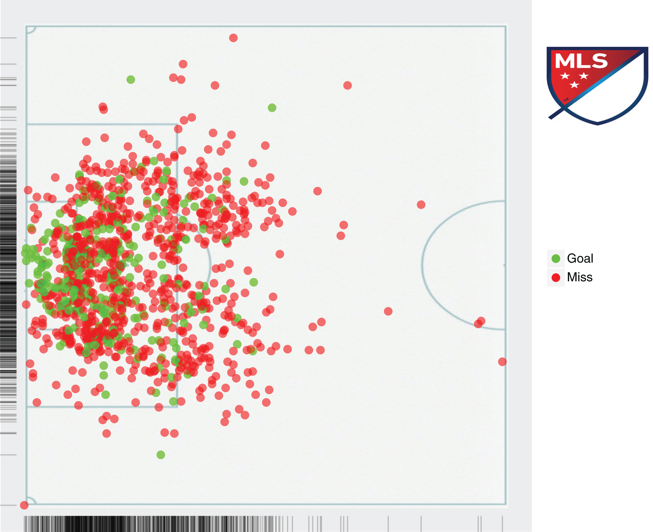
Fig. 1
A shotchart of the shots used in our analysis.
2.1Existing Literature
As aforementioned the notion of expected goals is not new. Soccer practitioners have developed their own models to estimate the expected goals from the shots taken from a team. The vast majority of these models utilizes features related to the distance from the goal line Bertin (2015), Chappas (2013), 11tegen11 (2014) in order to calculate the probability of a shot leading to a goal. Lucey et al. (2015) were the first to use player tracking data in order to include game context related features in their expected goals model. One of the gaps in the existing literature is that the goal probabilities obtained from the developed models are not (properly) evaluated. Typically the model evaluation includes accuracy figures and/or the average prediction error between the actual goals scored and the expected goals based on the shot model. Our current work fills this gap by highlighting an appropriate way to evaluate the probability output from a shot model. While we develop our model and evaluations using only features from shot charts - we do not have access to detailed tracking data - the probability evaluation approach we describe can be used for more elaborate models such as the one presented by Lucey et al. (2015).
In another direction, Vilar et al. (2013) focus on the analysis of local dynamics and show that local player numerical dominance is key to defensive stability and offensive opportunity, while Bar-Eli et al. (2007), Bar-Eli and Azar (2009) further collected information from 286 penalty kicks from professional leagues in Europe and South America and analyzed the decisions made by the penalty kickers and the goal keepers. Their main conclusion is that from a statistical standpoint, it seems to be more advantageous for a goal keeper to defend the penalty kick by remaining in the goal’s center. Furthermore, Di Salvo et al. (2007) analyzed the motion of 200 soccer players from 20 games of the Spanish Premier League and 10 games of the Champions League and found that the different positional roles demand for different work intensities.
Finally, similar line of research exists in hockey analytics where models for expected goals are developed in a similar manner Eric (2012), Johnson (2016), Perry (2016). In these models again the main features that determine the shot quality include the location of the player taking the shot as well as the type of the shot (e.g., wrist shot, slap shot, deflection, etc.).
2.2Dataset
For our study we compiled a set of 1,115 (non-penalty) shots from 99 MLS games during the 2016 regular season. The data were collected by watching and manually tagging the (x,y) coordinates of shots on target in each Major League Soccer game between March 6 - May 18, 2016. John Burn-Murdoch’s soccer pitch tracker was used to tag each shot’s location, outcome, game state, assist type, and to define the phase of play from which the shot came (i.e. set piece, open play, etc.) Burn-Murdoch (2015). The final annotated dataset includes the following tuple for each shot:
<ID, Player, Team, Opponent, Loc.X, Loc.Y, Outcome, Assist Type, Shot Type, Play Type, Angle, Distance>
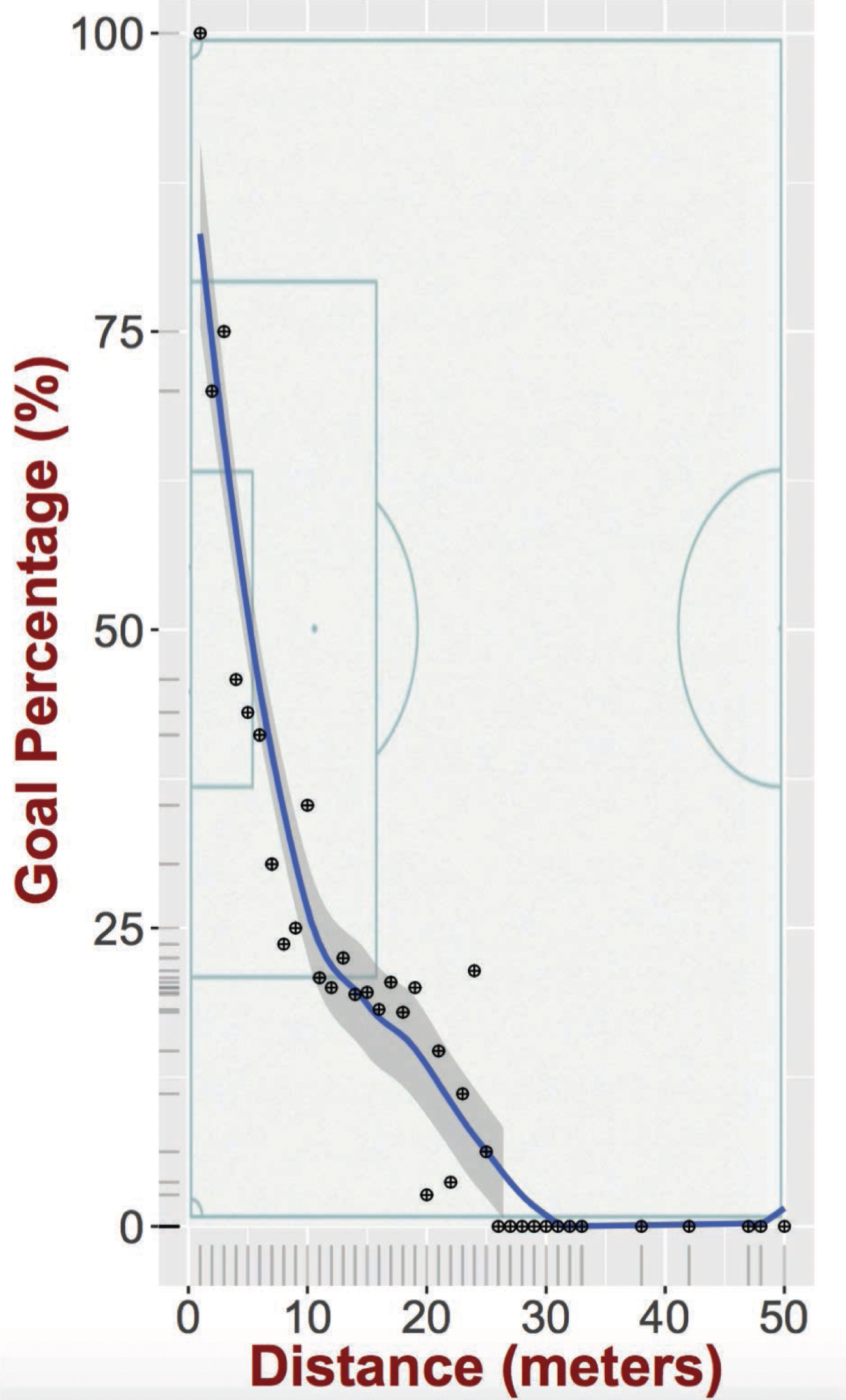
Figure 1 graphically depicts the shot chart for the whole dataset, while Fig. 2 visualizes separately the goals and missed shots as well as their spatial density. Before describing our model for the goal probability for each shot, we perform some basic analysis of the shots with respect to the features included in the shot tuple described above. Table 1 presents our results. As we can see there are not any statistically significant differences in the baseline goal probabilities when focusing on the different values for a given feature. For example, an open play and a set-piece play both have the same baseline probability of a goal. The same is true for a left, right or header shot. The only slightly statistically significant difference is observed when a player creates the shot on his own (i.e., self assist), in which case there is a lower baseline probability of scoring a goal. However, as we will see in the following section, these features do not bear any significant modeling power for the probability of success for a shot. Figure 3 further depicts the probability of a shot ending up to a goal as a function of the distance from the goal line. As one might have expected the further away the shot is taken from the goal line the less probable is to result into a goal.
Fig. 2
A location density for the shots that resulted in a goal (left figure) and the ones that were misses (right figure).
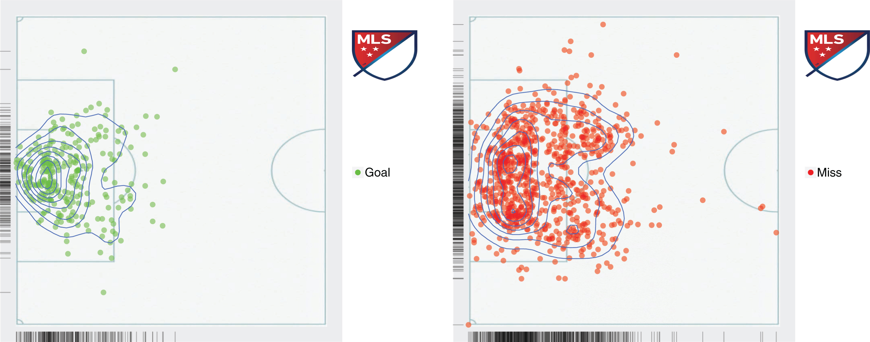
Table 1
Goal probability for different types of plays, assists and shots
| Type | Goal Probability (%) | 95% CI (%) | |
| Play | Open | 25.3 | 2.8 |
| Set-Piece | 24.1 | 6.5 | |
| Assist | Cross | 32.4 | 5.9 |
| Pass | 22.3 | 4.2 | |
| Self | 18.0 | 4.7 | |
| Other | 32.4 | 7.5 | |
| Shot | Header | 24.0 | 6.2 |
| Left | 24.4 | 4.7 | |
| Right | 25.8 | 3.5 |
3Models and Analysis
In this section we begin by presenting our goal probability model. Then we describe our expected goals model, while we finally explore the connection between offensive efficiency and the spatial distribution of a team’s shots through the lens of fractal dimension.
3.1Goal Probability Regression Model
In this section we will present our model for the probability of a shot leading to a goal, which will form the basis of our expected goals calculations. In particular, let us denote with Gs a binary random variable that represents whether shot s resulted in a goal (Gs = 1) or not (Gs = 0). Every shot s is associated with a feature vector zs that captures various attributes of the shot that we will describe shortly. We will use logistic regression to model the random variable Gs. The output of the model y provides us with the probability y = Pr [Gs = 1]. Hence, simply put, y is the probability of scoring a goal with shot s. The logistic regression model for G is given by:
(1)
The coefficient vector a includes the weights for each individual element of the input vector z, and is estimated using the shot data. The value of coefficient ai quantifies the relation of feature zi with the probability of scoring a goal (when keeping the rest of the factors included in the model constant), while the corresponding p-value quantifies its statistical significance. The features we use as the input for our model include:
Fig. 3
The goal percentage of shots as a function of distance from the goal line.
• Location information: This includes the coordinates - (x,y) - of the location that the shot took place.
• Distance: This is the distance of the shot location from the goal line.
• Shot angle: This is the angle created by the two straight lines connecting the shot location with each of the vertical goal posts.
• Shot type: This is a categorical variable that captures whether the shot was a header, a right or left leg shot.
• Assist type: This is a categorical variable that captures the type of assist that resulted to the shot.
• Play type: This is a categorical variable that describes whether the play was a set piece or an open play.
Table 2
Goal Probability Regression Model (Significance levels:†: 10% ∗: 5% ∗∗: 1%)
| Variable | Coefficient (Std. Err.) |
| Location x | 0.11 |
| (0.053) | |
| Location y | 0.017 |
| (0.013) | |
| Shot distance | -0.19* |
| (0.061) | |
| Shot angle | 0.023** |
| (0.006) | |
| Shot type (Header) | -0.15 |
| (0.407) | |
| Shot type (Left) | 0.36 |
| (0.408) | |
| Shot type (Right) | 0.36 |
| (0.407) | |
| Play (Set-Piece) | 0.0015 |
| (0.039) | |
| Assist (Pass) | -0.057 |
| (0.045) | |
| Assist (Self) | -0.042 |
| (0.051) | |
| Assist (Other) | -0.051 |
| (0.049) | |
| Intercept | -0.011 |
| (0.41) | |
| N | 1115 |
| AIC | 1165.2 |
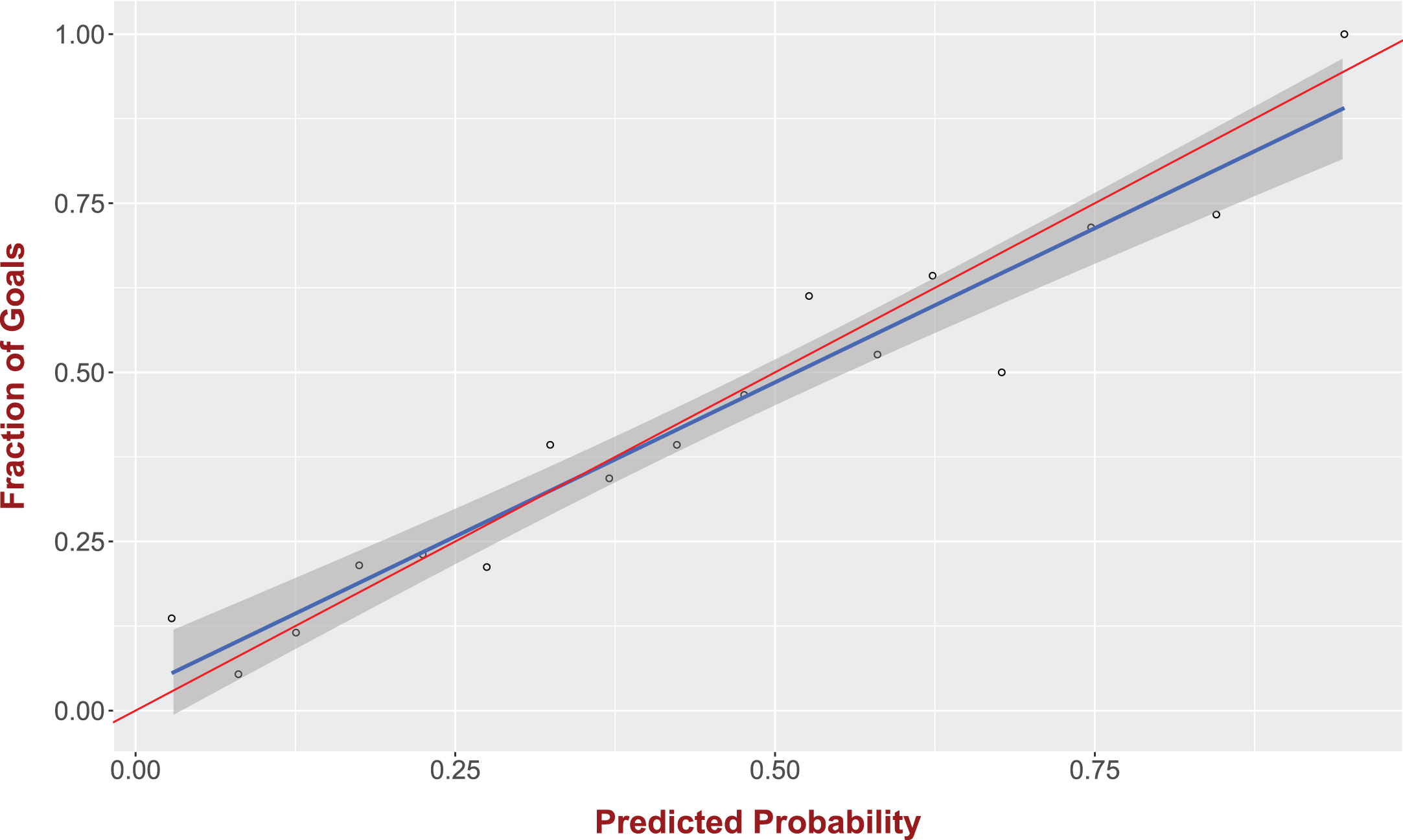
We trained the model with the shot data described in Section 2 and Table 2 presents our model. As we can see the distance from the goal and the angle of the shot are the only statistically significant features that impact the probability of a shot leading to a goal, while the type of shot, assist and play are not significant independent variables. A typical way to evaluate a logistic regression model is through its accuracy in predicting the output variable. In our case the prediction accuracy of the model is 77.2%. However, the purpose of using the above model is to calculate the expected goals based on the shots taken by a team or a player and not to predict whether a shot will result in a goal or not. In fact, the accuracy metric is rather misleading in this setting since given that only 25% of the shots end up to a goal the dataset11 is unbalanced Chawla et al. (2004); a deterministic model that predicts every shot to not be a goal will have a good performance with regards to accuracy - 75% in our dataset. On the contrary, the model’s accuracy of the predicted probability is our main evaluation criterion and not the model’s accuracy at predicting a goal. In order to evaluate the predicted probability, ideally we would like to have the same shot repeated several times. For example, consider a shot with a 30% probability of score. Then if the shot was taken 100 times - under the same conditions - one should expect approximately 30 of them to end up to a goal. However, this is obviously not possible to perform and hence, we rely in the following approach. In particular we will use all the shots in our dataset. If the predicted probabilities were accurate, when considering all the shots given a probability of x% being a goal, then x% of these shots should end up to a goal. Given the continuous nature of the probabilities we quantize them into groups that cover a 5% probability range. For higher predicted probabilities (> 0.7) we quantize the data to a 10% probability range given the small sample size within this range. Figure 4 presents on the y-axis the fraction of shots that ended up to a goal, while the x-axis corresponds to the predicted probability of goal. In order to avoid any biases in the estimation of the goal probability of a shot we used the leave-one-out approach, that is, for every shot s we used the rest of the data to train a model and then predict the goal probability for s. The blue line corresponds to the linear fit, while the shaded area is the 95% confidence interval of the fit. The red line is the y = x line (ideal case, i.e., perfect probability estimation). As we can see this line falls within the confidence interval, which translates to an accurate probability inference. The corresponding linear regression provides a slope with a 95% confidence interval of [0.77, 1.1] (R2 = 0.93) and a non-significant intercept (0.03, p-value = 0.39), which to reiterate means that we cannot reject the hypothesis that our data fall on the line y = x where the slope is equal to 1 and the intercept is 0.
Fig. 4
Our logistic regression model is providing accurate goal probabilities. For a given set of shots with predicted goal probability π the fraction of shots that resulted in a goal is also (approximately) equal to π.
Another metric that has been traditionally used in the literature to evaluate the performance of a probabilistic prediction is the Brier score β Brier (1950). In the case of a binary probabilistic prediction the Brier score is calculated as:
(2)
In conclusion, the model for the goal probability is accurate and well-calibrated (compared to the baseline climatology model).
3.2Expected Goals Model
Using the above model we can now estimate the number of expected goals of a team/player within a game or a span of games. Let us consider the set of shots
(3)
(4)
Fig. 5
Offensive and defensive efficiency of MLS teams as captured by the expected goals model.
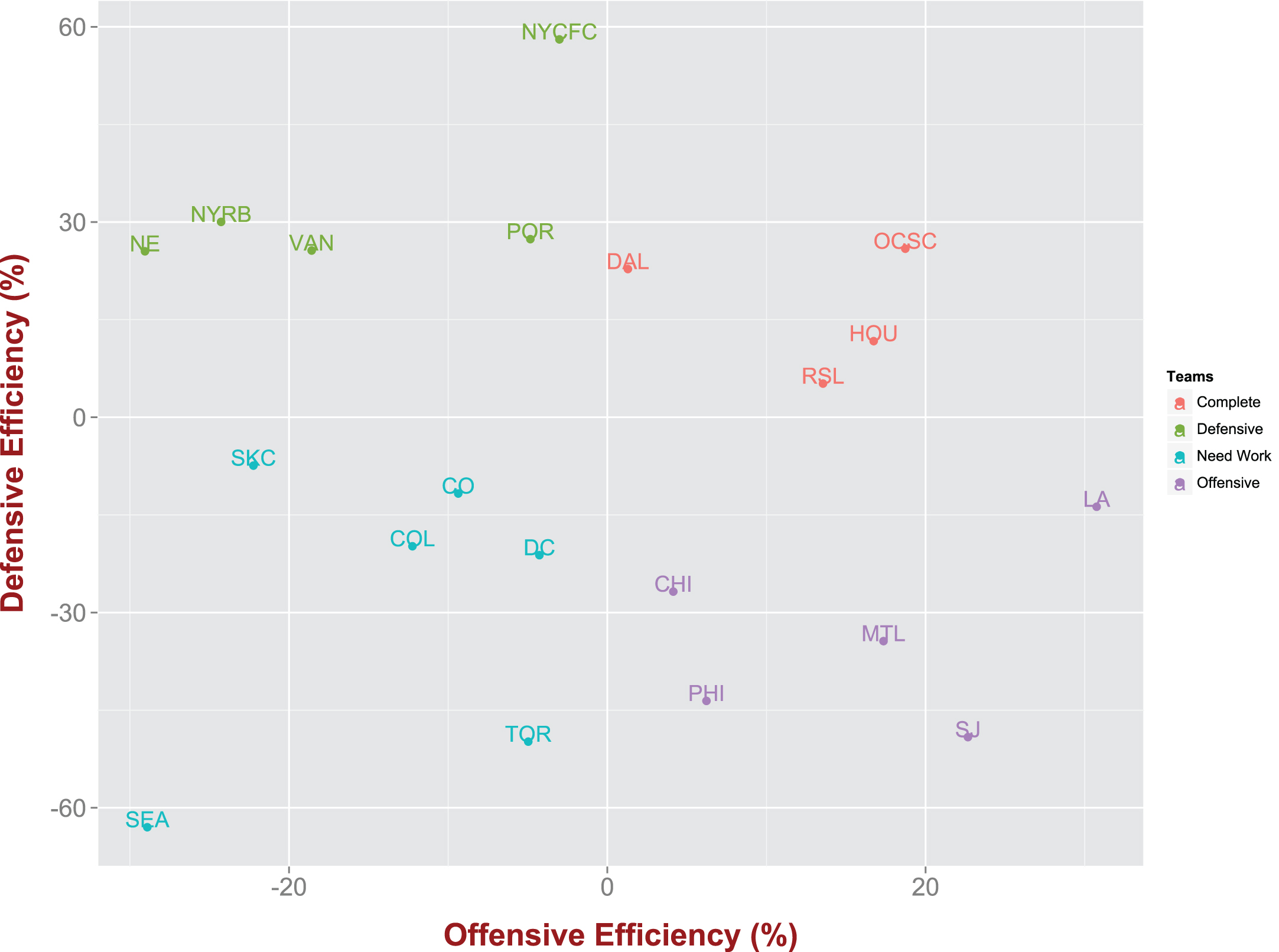
Using the expected goals as calculated above one can classify teams based on how much better/worse they actually perform over the expectation. This evaluation can be made for both the offense and the defense of a team. Formally, we have the following definitions:
(5)
(6)
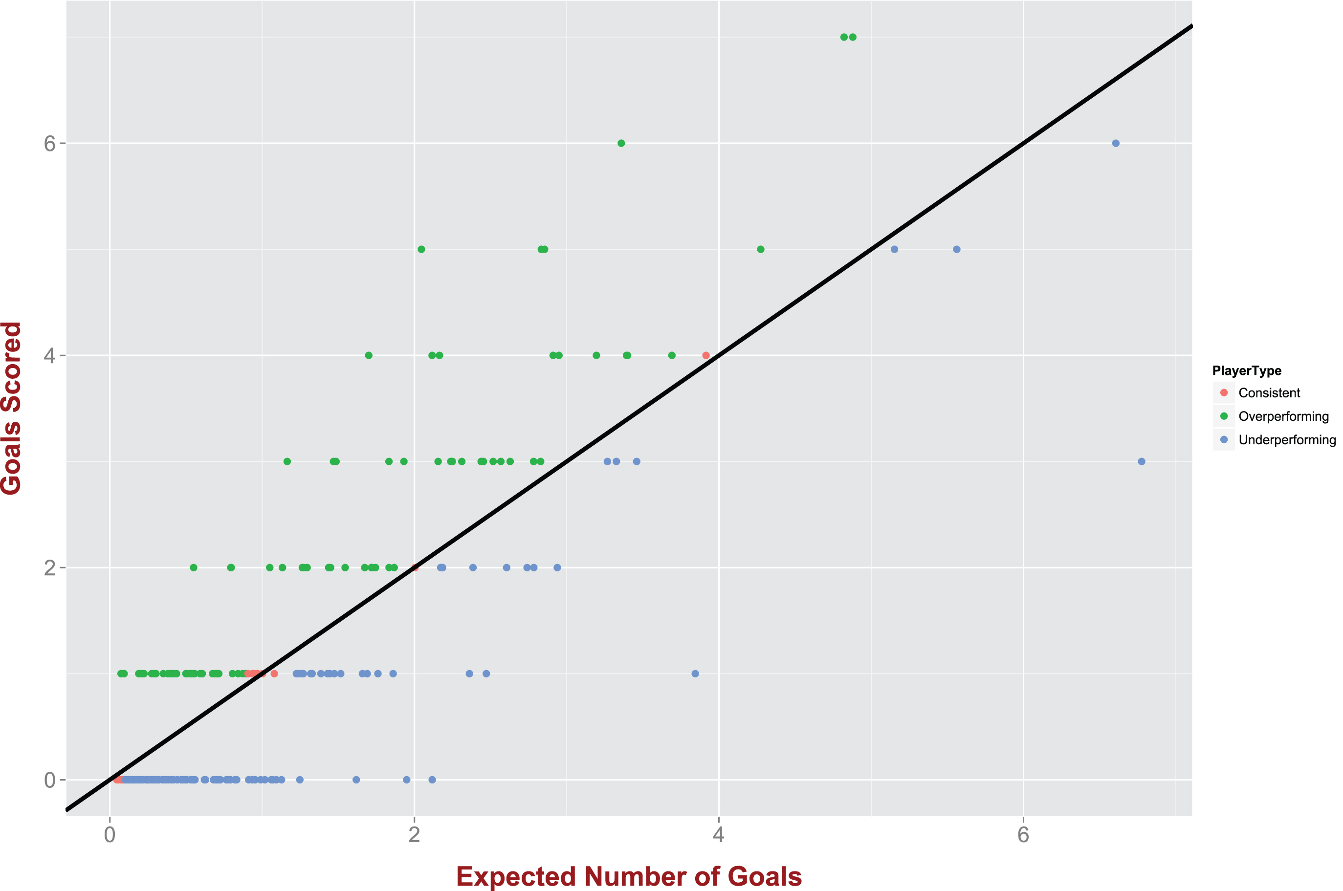
Fig. 6
Our expected goals model can help us classify players to “underperformers” and “overperformers”.
3.3Fractal Dimension and Offensive Efficiency
In what follows we want to examine whether there is any relationship between the spatial distribution of the shots taken and the offensive efficiency of the teams. In order to achieve this we need a metric that concretely describes the spatial distribution of a team’s shot in a condensed manner (e.g., through a single number). For that matter we will borrow the notion of fractal dimension from fractal theory. In particular, let us consider a set of points
(7)
An infinitely complicated set
Fig. 7
The empirical cumulative distribution of the MLS teams’ shot chart fractal dimension.
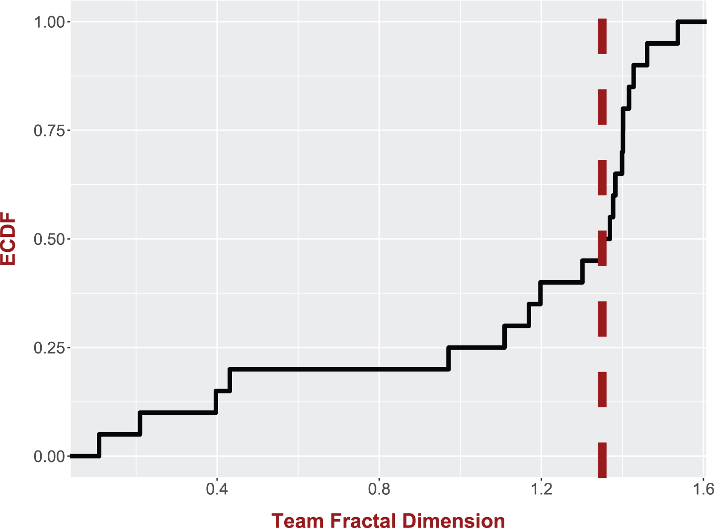
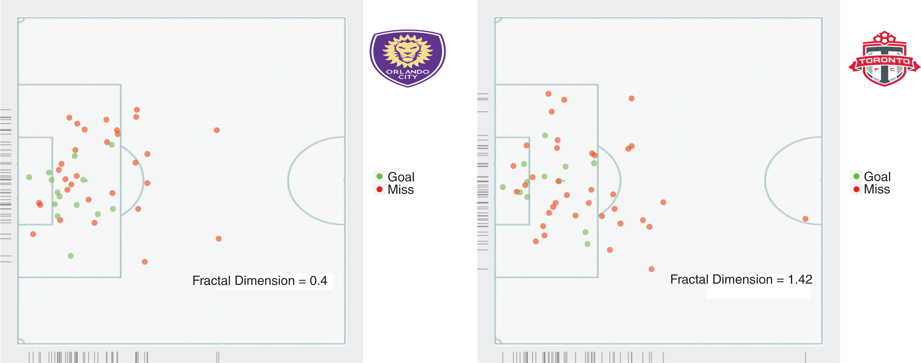
Fig. 8
A location density for the shots that resulted in a goal (left figure) and the ones that were misses (right figure).
In our case, the set
What these results seem to imply is that teams with higher offensive efficiency tend to utilize a smaller area on the field with regards to their shots. This might seem counter intuitive, since one might expect that taking shots from a variety of locations would stretch the defense more, create more open spaces and hence, create better situations for scoring. However, the opposite is true and one of the reasons might be the fact that a team by having its shots uniformly distributed over the space, will end up taking many low quality shots. Furthermore, the defenses are aware of the low chance of making a shot from a long distance and hence, the stretching of the defense is less than expected. Of course, the tactical strategy followed by a team’s offensive or defensive unit - and of course the spatial distribution of the team on the field - depends a lot on the talent on the team. For example, a defense that has to face a team with talented offensive players might want to give them space in the backfield in order to avoid one-to-one situations near the penalty area that can be a miss-match for the defense. This will end up in a situation similar to the one observed, i.e., non-stretched defenses that allow distant, low-probability, shots but try to close the spaces closer to the goal line by creating a denser defense in the high-percentage shot areas. Figure 8 depicts two representative cases of teams with small and high fractal dimensionality. As we can see while both teams take approximately the same number of shots, the Orlando City Soccer Club is much more efficient, since it distributes its shots over a smaller area, which is also the area of high quality shots (i.e., close distance to the goal).
4Discussion and Conclusions
In this study we have developed a model for quantifying the probability of scoring a goal based on features of the shot taken. We have particularly focused on ways for evaluating this model that go beyond the classification accuracy, which is secondary (if not irrelevant) from a player/team evaluation perspective. More specifically, we focus on the calibration of the predicted probabilities. We first group together shots with similar goal probability p as obtained from our model and we compare the fraction of shots from this group that ended up being scores with p (ideally the these two should be equal), while we also use the Brier score. We then utilize the model for the probability of a goal in order to calculate the expected number of goals for a team or a player. This allows us to develop efficiency metrics for the offense and the defense of MLS teams. Finally, we showcase how we can use ideas borrowed from complex systems theory to analyze spatial soccer data. In particular, we use the notion of fractal dimension that describes the distribution of a spatial set of points over the space and we see that teams whose shot charts exhibit smaller fractal dimensionality are in general associated with higher offensive efficiency. We further hypothesize that this is due to a careful selection of their shots from spots with high goal probability. On the other hand, teams with high fractal dimensionality, spread their shots more uniformly across the field and this will inevitably lead to many shots of low quality that are essentially “wasted” opportunities.
Shot charts is one only aspect of spatial soccer data. We believe that the notion of fractal dimension can also be useful in evaluating individual players with regards to their movement on the field. Tracking technologies allows us today to have a full spatiotemporal trajectory of players during the course of a game. When applied on trajectory data - both spatial and temporal information is present - fractal dimension can provide more insights, such as, whether the trajectory includes frequent short, “wandering”-like parts creating a bursty pattern Matsubara et al. (2013). This information can be useful for the analysis of many sports for which the spatio-temporal movements of players are important. For example, the fractal dimension of the ball trajectory has been used to quantify ball movement in basketball and has been shown to correlate with the outcome of a possession Pelechrinis (2017). We envision our study to trigger more research in the connection between complex systems theory and sports.
Notes
1 Our model includes only shots on target and this is why this percentage might appear even higher than what one might have expected.
References
1 | 11tegen11, (2014) . Expected goals 2.0 ? some light in the black box. http://11tegen11.net/2014/08/07/expected-goals-2-0-some-light-in-the-black-box/. Accessed: 2016-12-31. |
2 | Bar-Eli M. and Azar O.H. , (2009) . Penalty kicks in soccer: Anempirical analysis of shooting strategies and goalkeepers’preferences, Soccer & Society 10: , 183–191. |
3 | Bar-Eli M. , Azar O.H. , Ritov I. , Keidar-Levin Y. and Schein G. , (2007) . Action bias among elite soccer goalkeepers: The case ofpenalty kicks, Journal of Economic Psychology 28: , 606–621. |
4 | Bertin M. , (2015) . Why soccer’s most popular advanced stat kind of sucks. http://deadspin.com/why-soccers-most-popular-advanced-stat-kind-of-sucks-1685563075. Accessed: 2016-12-31. |
5 | Brier G.W. , (1950) . Verification of forecasts expressed in terms of probability, Monthly Weather Review 78: , 1–3. |
6 | Burn-Murdoch J. , (2015) . Football (soccer) pitch tracker. http://johnburnmurdoch.github.io/football-pitch-tracker/. Accessed: 2017-02-02. |
7 | Chappas C. , (2013) . Goal expectation and effciency. http://statsbomb.com/2013/08/goal-expectation-and-efficiency/. Accessed: 2016-12-31. |
8 | Chawla N.V. , Japkowicz N. and Kotcz A. , (2004) . Editorial: Special issue on learning from imbalanced data sets, ACM Sigkdd Explorations Newsletter 6: , 1–6. |
9 | Di Salvo V. , Baron R. , Tschan H. , Calderon Montero F.J. , Bachl N. and Pigozzi F. , (2007) . Performance characteristics according to playing position in elite soccer, International Journal of Sports Medicine 28: , 222. |
10 | Eric T. , (2012) . Shot quality & expected goals. http://nhlnumbers.com/2012/6/26/shot-quality-revisited-a-look-at-the-correlation-between-scoring-chances-and-shot-totals. Accessed: 2016-12-31. |
11 | Johnson D. , (2016) . Evaluating player evaluation metrics and expected goal models. http://hockeyanalysis.com/2016/03/03/evaluating-player-evaluation-metrics-and-expected-goal-models/. Accessed: 2016-12-31. |
12 | Lucey P. , Bialkowski A. , Monfort M. , Carr P. and Matthews I. , (2015) . “quality vs quantity”: Improved shot prediction in soccerusing strategic features from spatiotemporal data, 9th Annual MIT Sloan Sports Analytics Conference. |
13 | Mason S.J. , (2004) . On using “climatology” as a reference strategy in the brier and ranked probability skill scores, Monthly Weather Review 132: , 1891–1895. |
14 | Matsubara Y. , Li L. , Papalexakis E. , Lo D. , Sakurai Y. and Faloutsos C. , (2013) . F-trail: Finding patterns in taxi trajectories, Pacific-Asia Conference on Knowledge Discoveryand Data Mining. Springer, pp. 86–98. |
15 | Pelechrinis K. , (2017) . The athlytics blog: Measuring the immeasurable in basetball. http://wme/p7uVLS-Ey. Accessed: 2017-03-25. |
16 | Perry E. , (2016) . Shot quality & expected goals: Part 1. http://www.corsica.hockey/blog/2016/03/03/shot-quality-and-expected-goals-part-i/. Accessed: 2016-12-31. |
17 | Vilar L. , Araújo D. , Davids K. and Bar-Yam Y. , (2013) . Science of winning soccer: Emergent pattern-forming dynamics inassociation football, Journal of Systems Science and Complexity 26: , 73–84. |


