
Uncovering the sources of team synergy: Player complementarities in the production of wins
Abstract
Measuring the indirect effects on team performance from teammate interactions, or team synergy, has proven to be an elusive concept in sports analytics. In order to shed further light on this topic, we apply advanced statistical techniques designed to capture player complementarities, or “network” relationships, between teammates on Major League Baseball teams. Using wins-above-replacement metrics (WAR) over the 1998-2016 seasons and spatial factor models embodying the strength of teammates’ on-the-field interactions, we show that roughly 40 percent of the unexplained variation in team performance by WAR can be explained by team synergy. By building a set of novel individual player metrics which control for a player’s effect on his teammates, we are then able to develop some “rules-of-thumb” for team synergy that can be used to guide roster construction.
1Introduction
A whole that is greater than the sum of its parts: This aphorism is often used in sports to rationalize how a team made up of seemingly inferior players manages to outperform a superstar-laden team that looks unbeatable on paper. The movie Miracle features a scene in which U.S. men’s Olympic hockey team head coach Herb Brooks, facing skepticism about his chosen roster, tells his assistant coach, “I’m not looking for the best players, Craig. I’m looking for the right ones.” (Guggenheim, 2004). At its heart, this statement captures the dilemma faced by every professional sports executive in constructing a team roster. What defines the “right fit” of players, however, can often be very subjective. Here, we provide a formal definition based on the complementarity of player skill sets in the production of team wins via the interconnectedness of Major League Baseball (MLB) teammates’ on-the-field interactions.
Evaluating the degree to which a variety of inputs – in our case, different position players on a sports team – are complementary or substitutable in production (e.g. of team wins) is a topic that economists have wrestled with for just under a century (Hicks (1932) and Robinson (1933)). We appeal to this tradition and apply advanced statistical techniques designed to capture “network” relationships in order to measure the degree of team synergy through nonlinear effects in the on-the-field performance interactions of teammates that are characteristic of player complementarities. Finding a large degree of complementarities across players on the same MLB team provides scope for the hypothesis that these synergies play a fundamental role in team success in baseball. Similarly, finding individual players whose presence routinely complements their teammates allows for the identification of its sources.
The basis for our analysis is the correlations across teammates in their wins-above-replacement (WAR) metrics and their relationship to team wins. WAR calculations, like those made by FanGraphs and Baseball-Reference, provide a comprehensive measure of individual player performance. While these measures often differ in some key assumptions, central to each is the belief that a player’s actions should be judged regardless of the game situations in which they occur. By making context-neutral evaluations, WAR has the advantage of judging players solely on the aspects of team outcomes over which they have direct control (Cameron, 2017). A consequence of this assumption is that while WAR measures a player’s performance by how many wins a player is expected to contribute to his team above replacement level, it will not necessarily correspond to the actual contribution he made to team wins.
This discrepancy between WAR and team wins has been at the center of critiques of its value as a statistical tool for player evaluation. An oft-cited example is whether a player performed relatively well or poorly in so-called “high-leverage” situations (James, 2017). WAR may arguably lead to misleading judgments of a player’s ex-post value to his team in such confounding circumstances where a mismatch between team wins and aggregate team WAR can result. In fact, other researchers have used this mismatch to construct measures of “clutchness” which aim to back out the context-relevant portion of team wins (Sullivan, 2015). Similarly, aggregate team WAR may also fail to reflect a player’s full contribution to his team depending on the manner in which his interactions with teammates aids in the production of team wins. In this paper, we find that the mismatch between team wins and team WAR serves as a valuable empirical regularity for understanding the nature of team synergies in baseball.
We begin our analysis by using the WAR metrics produced by FanGraphs and Baseball-Reference to construct player productivity residuals for the 1998-2016 seasons. These residuals reflect the difference between the expected and actual number of team wins that can be attributed to each player in a given season. When aggregated across teammates, they measure the difference between a team’s actual win count and its expected wins based solely on individual player performances. If WAR was a comprehensive measure of each players’ contribution to team wins and players were perfectly substitutable along this dimension, the residuals for each team would sum to zero. However, this is not the case, with roughly 20 percent of the variation in wins across teams left unexplained according to our productivity residuals.
From this unexplained variation in the win-loss ledger of MLB teams, we then isolate the element of team wins arising from teammate interactions as opposed to potential mismeasurement in WAR stemming from other contextual factors. To measure the strength of teammate interactions, we take into account several dimensions of teammates’ on-the-field relationships, weighting more heavily pairings: 1) that play more often (taking into account both past and present playing time), and 2) that are characterized by the network relationships that exist between hitters in a team’s lineup and defensive positions. For instance, the correlations of the residuals of hitters who bat in adjacent positions at the top of the lineup are given more weight than the residual correlations of hitters who bat at the top vs. the bottom of the lineup. Similarly, the pitcher-catcher defensive relationship is given more weight than any other defensive pairing on the field in terms of measuring residual correlations across teammates.
Measuring teammate interactions in this way lends itself to the use of a spatial factor model to decompose our player productivity residuals into two separate unobserved components capturing elements of player complementarities. The first component identifies what we call character players, or players who positively influence their teammates regardless of the team that they play for; while the second component accounts for the role that a team’s management has on team performance to isolate what we call team players. This second component also makes it possible to capture a team’s historical ability to consistently turn individual player talents into extraordinary team outcomes, allowing for a relative ranking of MLB teams that can be used to measure organizations on the dimension of what we refer to as organizational culture.
Our methodology also has a natural connection to network statistics that allows us to construct refinements of WAR which isolate a player’s own contribution to team wins irrespective of his teammates, WAR-, and his contribution adjusted for his effect on his teammates, WAR+. Using WAR-, we demonstrate that roughly 40% of the unexplained variation in team wins by WAR is explained by player complementarities. We refer to this total network effect of a team’s players as tcWAR, or team complementarity WAR, and provide examples of over- and under-achieving teams in recent seasons. Similarly, using WAR+, we show that WAR tends to overvalue the contribution of low impact players and undervalue the contributions of high impact players to team performance. A player’s net impact on his teammates, i.e. WAR+ - WAR, is then what we refer to as his pcWAR, or player complementarity WAR. Our analysis of pcWAR confirms the conventional wisdom that star players tend to make their teammates better.
Our tcWAR estimates indicate that it is fairly rare for a team to over-achieve in terms of team synergy; and, furthermore, those teams that do demonstrate very little persistence on this dimension. In this respect, we find that synergy may be accurately described as “catching lightning in a bottle,” and is an aspect of team performance that must be closely monitored and constantly managed. We then identify organizations that have exceeded and fallen short of expectations on this dimension. In addition, we show that the highly mean-reverting properties of team synergy are something that can be exploited by teams to improve upon pre-season team win projections. For example, using out-of-sample projections of tcWAR we demonstrate that it would have been possible to improve upon PECOTA pre-season projections for the 2008-2016 seasons by a statistically significant margin of roughly 1 win on average.
The effect that player complementarities have on team synergy is shown to be much more persistent, with pcWAR lending itself more easily to prediction than tcWAR. However, we document that this persistence is highly nonlinearly related to past player performance, with persistence increasing in the talent level of the player (e.g. “Star” players exhibit nearly five times the persistence as “Scrub” players and about 1.5 times as much as “Role” players as defined by the player’s previous season WAR). This suggests that player complementarity expectations based on past performance may be an appropriate guide for teams to judge their own players. We then identify players in our sample who have exceeded or fallen short of expectations on this dimension. Finally, we break down our pcWAR metric into separate components due solely to characteristics of the player versus other contextual factors related to their team, the former of which could be used as well to guide teams looking to alter their synergy profile through trades or free agency.
To provide further convenient “rules-of-thumb” for general managers in order to maximize team synergy in roster construction, we next construct age-position profiles for pcWAR conditional on the dynamics discussed above and player and team characteristics. For example, we show that the conventional wisdom that older players make for good teammates has support empirically, but the rate of development of team synergy-related skills varies by position. Our profiles also allow for the estimation of a player’s Intangibles, defined by whether or not their pcWAR exceeds or falls short of their profile. Using this measure, we quantify the “David Ross Effect,” so-named after the back-up catcher who we show outperformed his complementarity profile for much of his career.
The identification of players such as David Ross represents a potential source of competitive advantage for MLB teams. Using player salary data, we show that MLB teams have in the past inconsistently valued the team synergy-related skills that we capture in our pcWAR metric. Only during a player’s free agency years does his compensation positively reflect on average his contribution to team synergy after controlling for various other individual factors such as his WAR, age, and experience. Furthermore, MLB teams have placed too low of a value on the Intangibles element of pcWAR than the value of a win in MLB would suggest is appropriate. One possible explanation for this would be an inability to identify and measure this element of team synergy, a feature which our analysis overcomes.
The remainder of this paper proceeds as follows: Section 2 provides a brief summary of the relevant literature. Section 3 describes our methodology for measuring team synergy. Section 4 then details our refinements of WAR, and section 5 presents rules-of-thumb for roster construction. Section 6 then concludes and offers some possible extensions of our methodology.
2Literature review
Accurately measuring the effects of teammate interactions broadly considered has in the past been referred to as the “holy grail” of performance analytics (Schrage, 2014). Unsurprisingly, then, a number of other researchers have already made attempts to define and measure the importance of various types of player interactions as they relate to team performance in MLB. Their efforts have often focused on identifying the particular traits that denote good “clubhouse culture,” and how this translates into success on the field. Levine (2015) suggests that the presence of a charismatic leader on a roster could have an outsized effect on the performance of his teammates. Similarly, Phillips (2014) uses a regression model and estimates that compositional effects can account for up to four wins in a regular season based on roster characteristics like wage parity and demographic variation. Carleton (2013) focuses on two particular players, Brandon Inge and Jonny Gomes, who have been suggested as “good chemistry” players by teammates. He attempts to isolate whether their roster presence affected their teammates’ productivity relative to their expectation for a variety of performance measures. Others have even suggested physiological underpinnings to the performance relationships exhibited in the interactions of teammates (SyncStrength, 2016).
In contrast, economists have generally focused more on the particular mechanisms that may generate productivity spillovers between teammates, framing the problem as one of players serving as complementary inputs in the production of team wins. The degree of complementarity across players varies substantially across the major professional sports leagues. On one extreme, basketball is a sport where “star” players often have the ability to substitute for their less talented teammates. To this point, only two of the top ten players as measured by Hollinger’s individual PER metric for the 2016-17 NBA season played for teams that did not make the playoffs. On the other extreme, football presents itself as the quintessential team sport, as it requires more players coordinating their efforts on the field of play.1 Baseball, on the other hand, seems to fall somewhere in the middle, with some observers noting its largely individualized nature and others highlighting the importance of offensive and defensive interactions. For instance, Gould and Winter (2009) find that the performance of batters increases with that of other batters on a team. Arcidiacono et al. (2017) suggest that this may be the case because pitchers tend to throw fewer balls to avoid a walk based on the hitting ability of subsequent batters. On the defensive side of the ball, Willis (2017) provides the example of a strong fielding shortstop that may produce greater value to his team if its pitching staff tends to induce ground balls from opposing batters.2.
The primary difficulty that others have faced when trying to quantify the importance of these interactions in MLB has been their focus on identifying a priori the individual factors that drive it. Our methodology is instead designed to look for correlated “mistakes” in the relationship between team wins and the wins-above-replacement (WAR) metrics of teammates which can tell us something about the complementarities inherent to roster construction. The strength of using WAR for this purpose is its comprehensive nature: It compresses all of the things that a player can do to help his team win at the plate, in the field, or on the mound into one number. We concede, however, that WAR statistics are not perfect.3 For example, there are two predominant WAR methodologies (fWAR and bWAR) that can in some extreme cases lead to quite different valuations of a player’s worth. Both FanGraphs (fWAR) and Baseball-Reference (bWAR), however, have taken steps to standardize their particular calculations of WAR such that the definition of a “replacement level” player is the same across both methods (Cameron, 2013). As Miller (2016) notes, the remaining differences in methodology lie in the more subjective choices necessary to make the type of comprehensive valuations to which wins-above-replacement aspires, such as whether a pitcher’s quality should be reduced to the outcomes (i.e. runs) for which he is ostensibly responsible or if it should take into consideration how luck and fielding quality may influence these outcomes.
Rather than focus on the details of these differences in methodology, most criticisms of WAR instead center around the general wins-above-replacement paradigm of translating expected runs into wins in a way that ignores how context may affect team outcomes – for example, a bases-loaded single counts the same as one with two outs and no runners on base. Such critiques hew closely to common conventions regarding “clutchness,” or whether or not certain players are more capable than others in high leverage situations. Sullivan (2015) notes that while little evidence exists for within-season variation of “clutch” performances being driven by particularly capable teams or players, timing can still be an important factor in explaining how teams may outperform their expectations based on metrics like WAR. In this spirit, it is worth emphasizing then that our particular use of WAR is intricately linked to a similar notion that individual players’ performances cannot be measured in isolation, and instead often depend critically on the performance of the players around them. This stands in contrast to the other vein of criticism that WAR contains some glaring omission of an activity a player engages in to contribute to a team’s success. While our analysis would surely be influenced by shortcomings like the latter, its ultimate goal is in uncovering shortcomings like the former. We are not interested, however, in the context of how individual play impacts team performance, but instead the correlated nature of performances arising from on-the-field teammate interactions.
3Measuring team synergy
In this section, we provide a formal definition for team synergy in MLB and outline our methodology for measuring it. Our first step along this path is to construct player productivity residuals capturing the difference between the expected number of team wins arising from a player’s performance relative to how many games that player’s team actually won.4 To measure a player’s performance, we make use of wins-above-replacement, or WAR, an advanced sabermetric that captures how many total wins a player contributes to his team above a replacement level player at the same position (Baseball-Reference (2013) and FanGraphs (2016c)). With these measures in hand, we then move to modeling performance interactions between teammates, or player complementarities, and the effect that they have on team performance. Finally, in order to account for the discrepancies among different WAR calculations mentioned before, we conduct our analysis separately using the WAR metrics produced by both FanGraphs, fWAR, and Baseball-Reference, bWAR. Both sources calculate WAR using the same replacement level (Cameron, 2013). This feature allows us to treat the results from the respective versions of our model analogously, as any differences between the two will only arise from the various ways that each calculation assigns WAR above replacement level.
3.1Player complementarity
To demonstrate what we mean by team synergy, consider the hypothetical relationships on a baseball team displayed in Fig. 1. For each panel, we display—through several contour lines—the mix of player talents across two particular positions on a baseball team holding the number of team wins fixed (where darker lines moving towards the northeast signify increases in team performance).5 On any contour line, the slope at a particular point denotes the increase (decrease) in WAR required at one position to displace a loss (increase) in WAR at the other position in order to hold overall team performance constant. The degree to which players are substitutable or complementary determines the curvature of these contour lines.
Fig.1
Hypothetical complementarity of select player relationships by position or placement in the batting order in terms of wins-above-replacement (WAR). DH refers to designated hitter, SP references starting pitcher, 2B is shorthand for second baseman, and SS denotes the shortstop position.
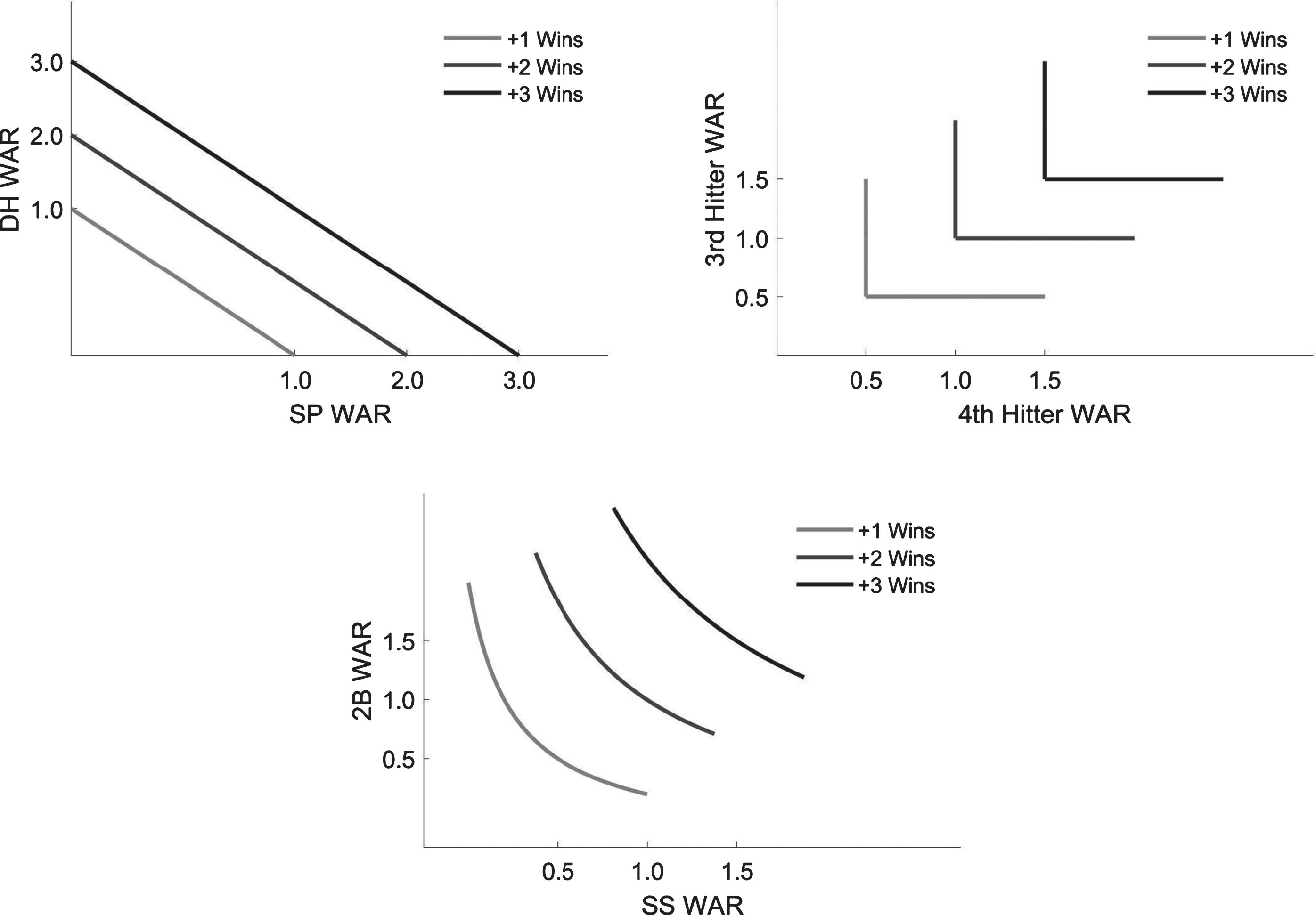
We propose that the stronger complementarities are among players the greater the scope that exists for team performances to be differentiated on the dimension of synergy. In the top left panel, we display what this relationship might look like for a designated hitter (DH) and a starting pitcher (SP) on the same team. Given that these two types of players will never find themselves on the field at the same time, and also engage in extreme types of activities, it’s natural to imagine that their performances are perfectly substitutable, consistent with the linear contour lines in this panel. In other words, for a team to achieve +2 wins (medium gray line) across their DH and SP positions they could obtain any combination of +2 WARs among the two positions. One possibility could be getting a strong +2 WAR designated hitter and a replacement level pitcher, or alternatively a strong +2 WAR starting pitcher and a replacement level designated hitter, or maybe a more evenly split +1 WAR at both positions. This sort of neutral interaction among players mirrors the implicit assumption underlying the construction of WAR values for teammates and how they map in the aggregate into a team’s WAR.
Now, consider the relationship between the 3rd and 4th place hitters in a team’s lineup, as displayed in the top right panel of the figure. For the 3rd and 4th hitters in a lineup, it is much more natural to assume that their performances are intricately linked when determining team performance. As good as the 3rd hitter might be (e.g. batting.300 and consistently getting on base), without a 4th hitter to either drive him in to score runs or protect the 3rd hitter from getting intentionally walked in pivotal hitting situations (e.g. runners on base with two outs), the team’s performance is likely to suffer. The complementary nature of these two players’ performances in dictating overall team performance is captured by the strong kinks in the contours displayed in this panel. For that same team to achieve +2 wins at the most cost-effective point, it will be important to have exactly a +1 WAR 3rd and +1 WAR 4th hitter. In this case, having a stronger (i.e. +2 WAR) 3rd hitter is only valuable in so much that the team has a capable 4th hitter to complement him. These sorts of complementarities are very certainly lost in the construction of WAR at the individual level and, thus, also by aggregating to the team level.
Of course, the 3rd and 4th hitter might be an extreme case as well. In the bottom panel, we instead display what might be the appropriate degree of complementarity between the second basemen (2B) and shortstop (SS). Here, one could imagine that some amount of substitution exists between these two defensive positions: a shortstop with incredible range might be able to cover up for a slow-footed second baseman in fielding ground balls up the middle. Alternatively, it would be natural to imagine that the two positions also have a degree of complementarity in that both of these players are also necessary for a team to successfully turn a double play. Furthermore, depending on where these two positions bat in the lineup, further offensive interdependencies may also come into play. Keeping with the notion of a team trying to accrue +2 wins across the two positions, this example is a balance of the previous two. While a +1 WAR second basemen and +1 WAR shortstop will yield +2 wins, a spectrum exists of the possible combinations of WARs across the second basemen and shortstop that would still yield +2 wins for the team. Note this spectrum is not as interchangeable as the hypothetical relationship between the starting pitcher and designated hitter, but some substitutability does exist unlike the hypothetical 3rd and 4th hitter relationship. Importantly, however, even the more moderate degree of interdependency displayed in this panel would not be captured in the construction of WAR.
3.2WAR and team wins
Instead of building a structural model of how individual players contribute to the different outcomes through the course of a game and then how these outcomes translate into the likelihood of a team winning a game, we take a more aggregate (reduced form) approach. Specifically, we search for systematic correlations in the misspecifications of WAR across teammates by incorporating into our analysis how a team actually performed. If these misspecifications are systematic both across teams and individual players as teammate relationships change, our statistical model will attribute them to the player complementarities that must exist between teammates along the lines of what is described in Fig. 1.
We show here that this tends to manifest itself in the fact that simply summing the WAR values for a team across its players does not perfectly replicate its wins above those expected of a team comprised entirely of replacement-level players. To get a sense of exactly how important player interactions may be to team performance, we regressed the number of wins for each team on the sum total of its players’ WAR. Specifically, we ran linear regressions of the form
(1)
where Wnt is the number of wins of team n in season t and WARnt is the sum total of wins-above-replacement statistics for all players on team n in season t based on either FanGraphs or Baseball-Reference’s calculations.6.
The ɛnt in these regressions are what we call team productivity residuals. We refer to them as such because in many ways they represent the baseball equivalent of the famous “Solow residual” used in economics to measure the productivity of firms.7 An MLB team with a positive ɛnt was a team who out-performed, or won more games than what could be attributed to the sum of its individual player performances (or in economic terms, a firm that produced more output than the usage of its individual inputs would suggest). Alternatively, a team with a negative residual would be a team who despite perhaps having a number of strong individual performances (as measured by WAR) under-performed as it pertains to wins.
The results from these regressions using data from the 1998-2016 seasons, shown in Table 1, provide several insights. First, it is clear that the estimates of β are close to 1.8 This is intuitive given how both WAR metrics are constructed, but also allows us to confidently use the idea that increasing a team’s WAR should have a one-to-one relationship with their number of wins.9. Furthermore, the estimate for α in our regressions is just less than 50. This estimate, too, has a natural interpretation of being the number of wins one would expect a team full of replacement level players to accrue. At about 50, clearly a team with only replacement level players is far from an average, or 0.500 winning percentage, team. With that being said, it is consistent with the construction of these measures.
Table 1
Team Wins Regressions: 1998-2016
| FanGraphs | Baseball-Reference | |||
| (1) Team Wins | (2) Team Wins | (1) Team Wins | (2) Team Wins | |
| Team WAR | 0.996 | 0.941 | ||
| (0.017) | (0.029) | |||
| Team WAR- | 1.030 | 0.933 | ||
| (0.014) | (0.024) | |||
| Constant | 47.691 | 48.150 | 49.569 | 51.404 |
| (0.649) | (0.538) | (1.071) | (0.890) | |
| R2 | 0.799 | 0.887 | 0.804 | 0.876 |
| Pseudo R2 | 0.789 | 0.873 | 0.793 | 0.867 |
| Observations | 570 | 570 | 570 | 570 |
Bootstrapped bias-corrected and accelerated standard errors clustered on team shown in parentheses based on 500 replications. Pseudo R2 is calculated as the average from a 57-fold cross-validation with recursive estimates of WAR- included in specifications (2).
The team productivity residuals,
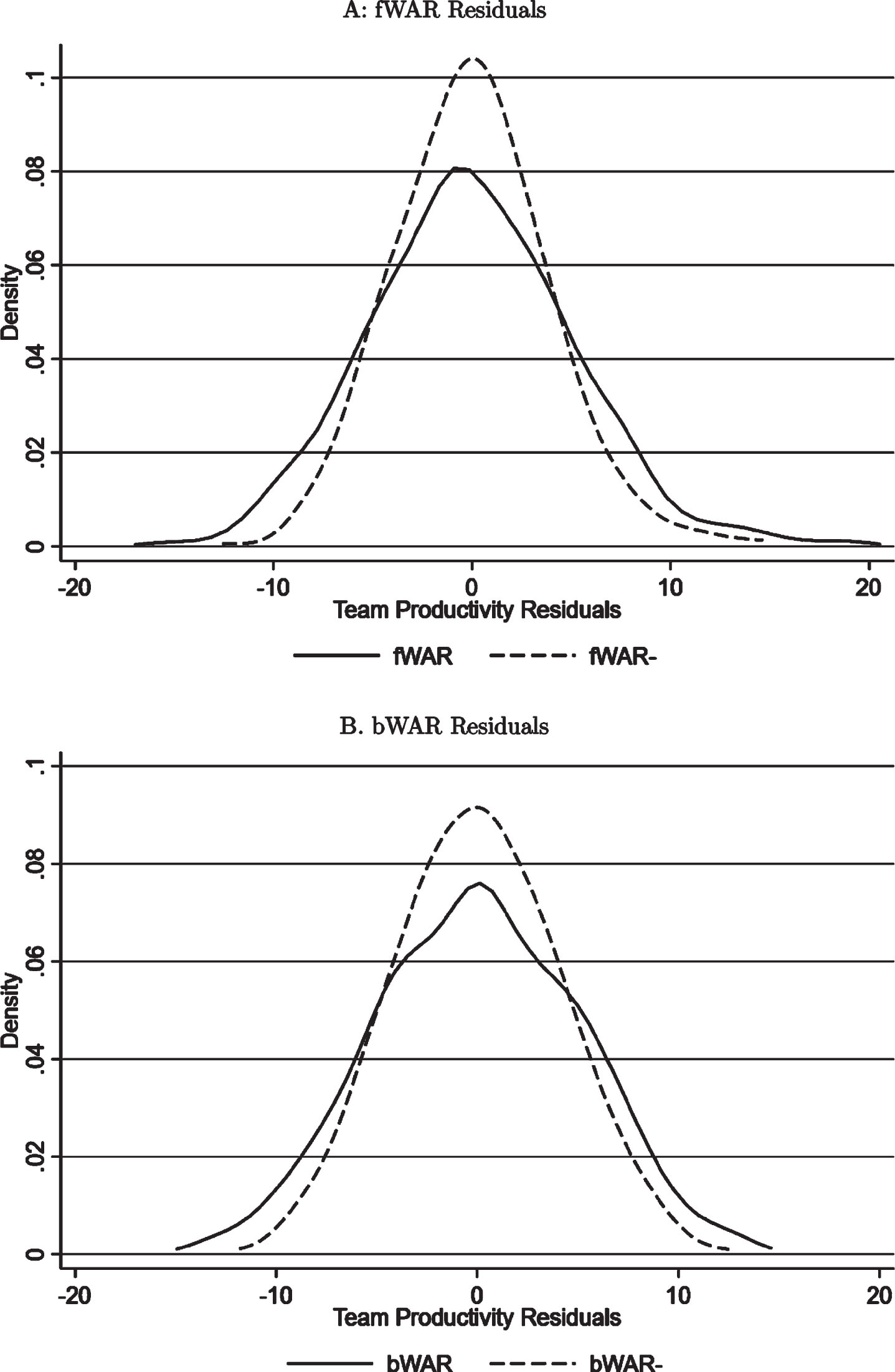
Fig.2
Kernel densities of team productivity residuals for various measures of wins-above-replacement (Fangraphs (fWAR) - panel A, Baseball-Reference (bWAR) - panel B) and our WAR- metrics.
To see why, consider the following interdependencies captured in our regression. In constructing a roster, teams face a problem of maximizing wins, W, subject to a payroll constraint and MLB regulations like the luxury tax. Suppose this production function, w, takes the form
(2)
where w takes as its inputs a team’s defensive and offensive production.1010 Defensive production is captured by d (f, p), a function that describes how fielding (f) and pitching (p) resources determine defensive value; and offensive production is captured by l (b), which specifies how batters (b) determine offensive value given a lineup configuration. If the team’s defensive ability depends upon the specific mix of fielding and pitching inputs, or if teams maximize the returns to their batter’s output based on their order in the lineup, then team synergy will be evident in the degree of substitution/complementarity between inputs.
We do not observe the functional form w takes for each team, but we do have the extensive work of sabermetricians to appeal to on this matter. In fact, the construction of WAR resembles this production function in many ways, as it incorporates fielding, pitching, and hitting metrics separately by converting them to run-equivalent values for each player which are then translated to team win values by using an historical run differential-win relationship. If the technology for turning player talents into team wins is linear with respect to the sum of its players’ individual WAR, i.e. if player performances are perfect substitutes, then the relationship below across the players (i) on a team in a given season should hold and the residuals of our regression should be zero in the absence of other contextual factors contributing to the deviation of team wins and team WAR.
(3)
However, if complementarities exist between teammates causing this relationship to be nonlinear, then our regressions will be misspecified.
When we replace WAR in our regressions with our measure that adjusts for the strength of teammate interactions, WAR-, this is exactly what we see. In this case, the higher R2 values of these regressions suggest that accounting for player performance interactions reduces the unexplained variation in team wins by roughly 40%. This remains the case even after we account for sampling variability and estimation uncertainty by examining the Pseudo R2 values from a k-fold cross-validation of these regressions.1111 The result of this adjustment on our team productivity residuals can be seen in Fig. 2. The kernel density of team productivity residuals using our WAR- measures (dashed lines) is much more concentrated than before with a standard deviation of about 4 wins and a range of about 25 wins.1212 Taken together, these results suggest that complementarities between individual players, or what we call team synergy, do indeed have scope for explaining some of the unexplained variation in team performance by WAR.
3.3Team wins and teammate interactions
Next, we focus on our methodology for decomposing team productivity residuals into player-specific productivity residuals. The basis for this decomposition is the following identity,
(4)
To arrive at this value, first we construct two weights designed to capture how a player’s placement in the batting lineup (lit) and his defensive position (dit) affect his expected contribution to team wins,
(5)
(6)
where Sijt denotes the number of times player i appeared in the jth slot of the lineup and gijt denotes the number of times player i appeared at each of the eight non-pitching defensive positions or pitcher/DH as a share of his total appearances.1313 The adjustment weights, bj and pj, then describe the relative importance weight given to their respective variables. Lineup weights are defined following Tango et al. (2007), while defensive position weights are defined following FanGraphs’ positional adjustment methodology (FanGraphs, 2016a) for fWAR and Baseball-Reference’s positional adjustment methodology for bWAR (Baseball-Reference, 2017). We then normalize each weighting scheme to sum to 1, with the resulting values reported in Table 2.
Table 2
Defensive and Lineup Position Weights
| FanGraphs | Baseball-Reference | Tango et al. (2007) | ||
| Defensive Position | d | d | Lineup Position | l |
| Catcher | 0.214 | 0.200 | 1 | 0.212 |
| First Base | 0.036 | 0.046 | 2 | 0.187 |
| Second Base | 0.143 | 0.150 | 3 | 0.162 |
| Third Base | 0.143 | 0.142 | 4 | 0.136 |
| Shortstop | 0.179 | 0.183 | 5 | 0.111 |
| Left Field | 0.071 | 0.067 | 6 | 0.086 |
| Center Field | 0.143 | 0.146 | 7 | 0.061 |
| Right Field | 0.071 | 0.067 | 8 | 0.035 |
| Pitcher/DH | 1/0 | 1/0 | 9 | 0.010 |
All weights are separately normalized to sum to one across fielders/pitchers and hitters.
In essence, with li and di we are skill-weighting the amount of time played at defensive positions and in the lineup in our calculations of the expected contribution to team wins. We use the Fangraphs or Baseball-Reference positional weights for this purpose, because they reflect a value judgement of the relative skill required to play each position holding fixed offensive skill. Similarly, we use the the Tango et al. (2007) lineup weights because they put a premium on time spent at the lineup positions that turn over more regularly throughout the course of a game. In this sense, they reflect the relative likelihood of getting additional plate appearances in a season, rather than any notion of proximity toward other players in the lineup.
With these weights in hand for each season, we then proceed to the construction of
(7)
where we refer to the product ηitτit as a player’s appearance weight in each season. FanGraphs and Baseball-Reference construct their WAR measures such that players contribute 1,000 WAR per 2,430 games league-wide (162 games for 30 teams), where, by construction, the offensive WAR contributions of pitchers sums to zero. The η in the above equation correspond to the proportion of league-wide fWAR/bWAR apportioned to position players and pitchers, respectively. This split is based on the assumption that because position players appear on both sides of the ball their contribution should be larger (FanGraphs, 2016a) as well as the relative split of salaries for free agent pitchers vs. hitters (Baseball-Reference, 2017). We maintain this assumption here, as it is also in keeping with the fact that we do not use offensive fWAR or bWAR data for pitchers in our analysis. To obtain τ, we use the sum of plate appearances (PA) and defensive outs (DOuts) for position players differentially weighted by the lineup and defensive position weights reported in Table 2. For pitchers, we use outs recorded (POuts) as we found it to be the most reliable measure for capturing the differences in pitching contributions across starters and a variety of relievers (middle relievers, closers, etc.).1414 Finally, we scale these inputs on a per-game basis, dividing plate appearances by a three appearance per-game scalar (3*162) and defensive and pitching outs by a 27 outs per-game scalar (27*162).
When aggregated across players on a given team in a given season, our player productivity residuals measure the difference between a team’s actual win count and what it would be expected to be based on the sum total of individual player performances as measured by WAR. Stacking these residuals into a player-season by team (IT × N) matrix
(8)
where A is an IT × IT network matrix identifying teammates in a given season. Typically, such a matrix is symmetric with 0’s on the diagonal and 1’s off the diagonal “connecting” teammates. However, in order to capture potential interdependencies in teammate relationships which correspond to their positions in the field and lineup, we replace the 1’s with weights αijt. For a pairing between player i and j playing for team n in season t, these connection weights are defined as follows:
This formalization of the network structure of our model captures several hypothesized features of teammate connections. First, the more one or both players in a pairing play, the more likely they will have played together and the stronger their on-field connection will be. Second, the implicit orderings of our lineup and defensive position weights shown in Table 2 capture specific on-field dynamics. If both players in a pairing tend to bat higher in the lineup, they will be more likely to affect each other’s performance based on the greater number of game situations they are expected to be a part of over the course of a season. Similarly, defensive pairings that include a catcher will be given relatively more weight, and if the other player is, for example, a middle infielder, this pairing will receive greater weight, all else equal, than one with a left fielder. Then, because pitchers receive a defensive weight equal to one, pitcher-catcher relationships will receive more weight than other position pairings, all else equal. Finally, to allow for added weight to be given to repeated “connections” across seasons in explaining player performance interactions, we sum over this value for each previous season in which the players were teammates.
Next, we assume that a factor structure exists for the panel SAR residuals, υ, such that player productivity residuals are summarized by a player-season specific component, or factors F, as well as a team-specific component, or factor loadings Λ. The F trace out a player’s career arc, potentially across several teams, and reflect whether that player finds himself among over- or under-performing teammates in each season. Identification of this latent variable is, therefore, predicated on roster turnover. Because of this, it will be more difficult in general for us to establish such a player vs. team breakdown the less roster turnover exists on a team over time. The Λ, on the other hand, reflect an organization’s average historical tendency to over- or under-perform relative to the collection of its players.
Solving for
(9)
where F is an IT × 2 matrix of our player-season factors and Λ is an 2 × N matrix of their team-specific factor loadings. To estimate this model, we use a two-step estimation procedure described in the Appendix. In the first step, an estimate of ρ is obtained by maximum likelihood conditional on a scale normalization on A. Given ρ, the factor model is then estimated by spatial principal components analysis (SPCA) to extract the latent player-season and team-specific components up to a scale normalization on Λ (Demsar et al. (2012)). In the next section, we provide further motivation for what we aim to capture in these factors in terms of team synergy.
4The network effects of playercomplementarity
To measure the interdependence of teammates’ performances, we borrow heavily from the social and economic network analysis literature (Jackson, 2008). Our spatial factor model fits the definition of a network. The players on a team in a given season make up the “nodes” of the network, with the strength of the connections between teammates summarized by our network matrix, factors, and their loadings. In other words, our model is simply a statistical framework for measuring the importance of correlations across team and teammate performances. In this section, we refine WAR in order to take into account these correlations; and, at the same time, construct new metrics that can be used to evaluate players’ contributions to team synergy.
4.1Sources of team synergy
Our methodology for measuring team synergy boils down to nothing more than a decomposition of the spatial correlation matrix of teammates’ productivity residuals into an exact linear combination of latent factors. To see this, consider that we can decompose our player productivity residuals into two parts: 1) a part that is unique to each player that we attribute to measurement error in team productivity residuals, and 2) a part that can be explained by each player’s interactions, or spill-overs, with his teammates that we attribute to team synergy, where the scalars w correspond to the entries of our spatial weight matrix Ω,
(10)
It is important to note here the role played by the measurement error term. In the absence of systematic spatial correlations in the player productivity residuals of teammates, this term will dominate our results. In this sense, it is an “out” for the model that allows it to explain the variation in player productivity residuals solely as a function of individual circumstances.1515 Based on our findings in Table 1, roughly 60% of the variance of the residual component between team wins and team WAR fits this description. The remaining 40% is what we then capture in the team synergy component.
We associate positive spill-overs with “good team synergy” and negative spill-overs with “bad team synergy.” We do not take a stance on what drives these spill-overs between teammates; and, in all likelihood, our latent factors probably capture a combination of many of the determinants of team synergy that others have already explored. However, by not restricting them ex-ante, they likely also embody elements of team synergy that could not be measured previously. The extent to which we do provide context for our factors is only to appeal to the work of other social scientists who have singled out certain psychological traits, such as “character” and being a “team player,” as being attributes of individuals in groups that excel in working together.
By allowing for two factors and restricting their loadings such that F = [ch, tp] and Λ = [l, λ], where l is a unit vector across teams, we can restrict our factor model to embody similar features.
(11)
We think of the factor ch as capturing a player’s innate character, as through this factor players demonstrate spill-overs to their teammates which do not depend on the identity of their team. In contrast, we think of the factor tp as capturing a player’s contribution that is more closely linked to the “match quality” of his current team (via λ), which we term as the team player factor.
Teams with large |λ| are then said to exhibit good organizational culture, as they either reinforce positive spill-overs (tp < 0 & λ > 0) or minimize negative spill-overs (tp > 0 & λ < 0) between teammates. Notice, however, that in our framework these factor loadings are fixed across time. As such, their estimation accounts for the vast majority of the uncertainty associated with our spatial factor model. For example, when a new season’s data is added to the model, the inference of λ applied to the previous seasons’ factor values for all current and former players on each team must be updated as a result. Looking at how estimates of λ evolve over time can then give a sense of changes in the model’s interpretation of an organization’s culture.
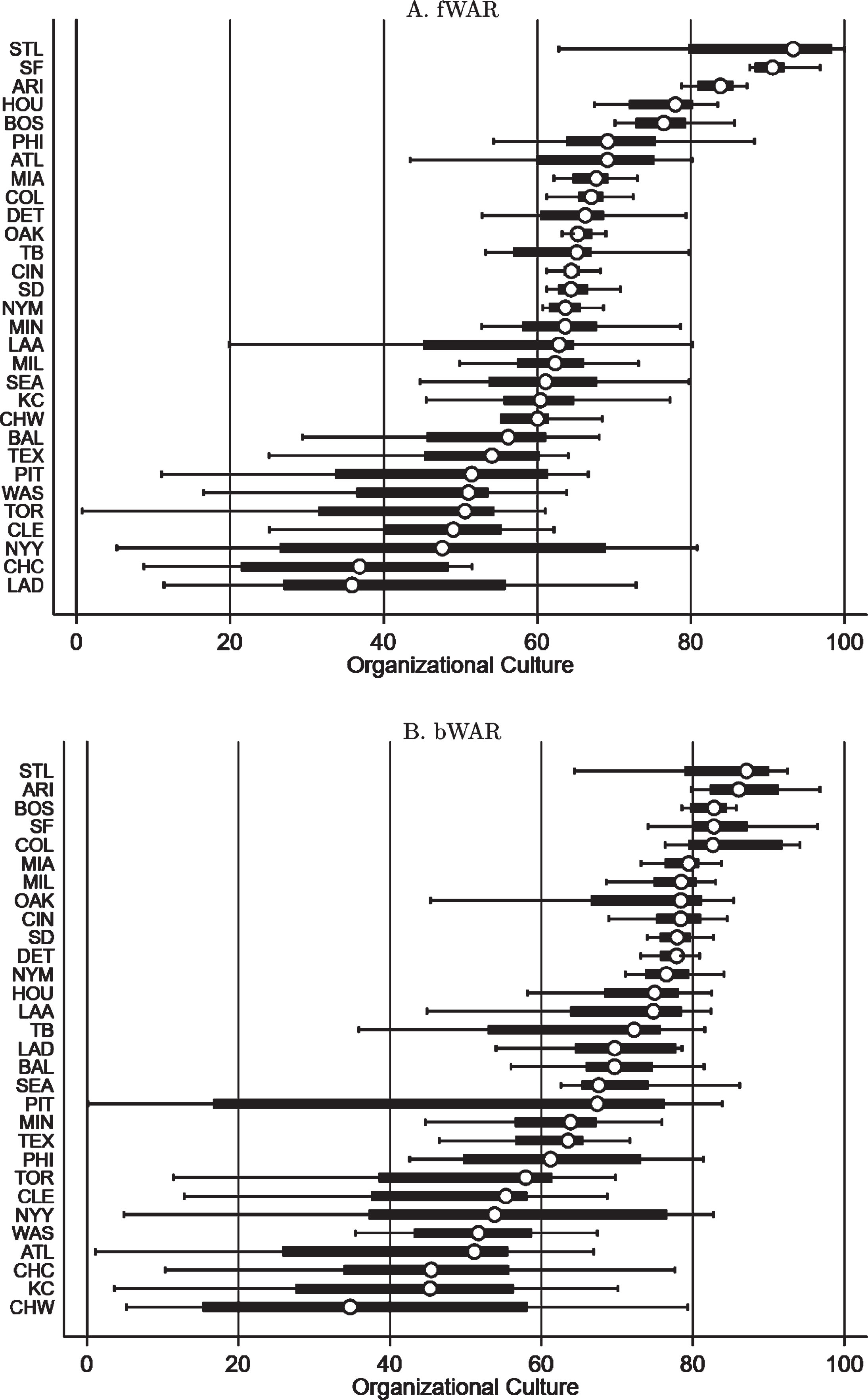
Figure 3 plots rankings from zero to 100 for all 30 MLB teams across the 1998-2016 seasons based on our estimated values of |λ| using both fWAR and bWAR data. To capture variation over time in these rankings the figure contains box and whisker plots for each organization summarizing the distribution of rankings obtained by estimating our spatial factor model “recursively” by adding one season at a time to the 1998 data. The dots in the figure correspond to the median ranking for each organization, while the bars give a sense of the interquartile range and broader sample variation over time. Certain organizations stand out along this dimension. For instance, the St. Louis Cardinals, Arizona Diamondbacks, and San Francisco Giants are in the top three of both rankings; while others do not fair nearly as well. Several organizations near the middle to bottom of the rankings, however, also exhibit a very large amount of variability over time, suggesting that for these organizations substantial changes in culture occurred during this time period.
Fig.3
Ranking of MLB organizations on the basis of our Organizational Culture metric for competing measures of wins-above-replacement (Fangraphs (fWAR) - panel A, Baseball-Reference (bWAR) - panel B). Organizations are ranked on a relative scale from 0 to 100, with 100 equal to the best organization over the 1998-2016 seasons. Dots denote the median ranking over this sample period for each organization, with box and whiskers summarizing sample variation.
4.2Team performance
If WAR measurements are indeed influenced by teammate interactions, then the regressions underlying our team productivity residuals are misspecified. Namely, WAR may be under- or over-counting the importance of individual contributions to team wins by ignoring the interactions between teammates. To adjust for this possible source of bias, we construct an alternative measure called WAR- which subtracts from the WAR of each player the portion of his productivity residual that can be explained by his teammates’ residuals. In network statistics, this is often referred to as the “in-degree” for a node.
(12)
Recall that Fig. 2 demonstrated the relative importance of adjusting WAR in this way for explaining deviations of team productivity residuals from zero. We can get a sense of the impact that this adjustment has on the productivity residual for any individual team by examining the aggregation of the differences between WAR and WAR- over teammates in each season. This is often referred to as the network’s “total-degree.” We call it “team complementarity wins-above-replacement,” or tcWAR, and scale it by
(13)
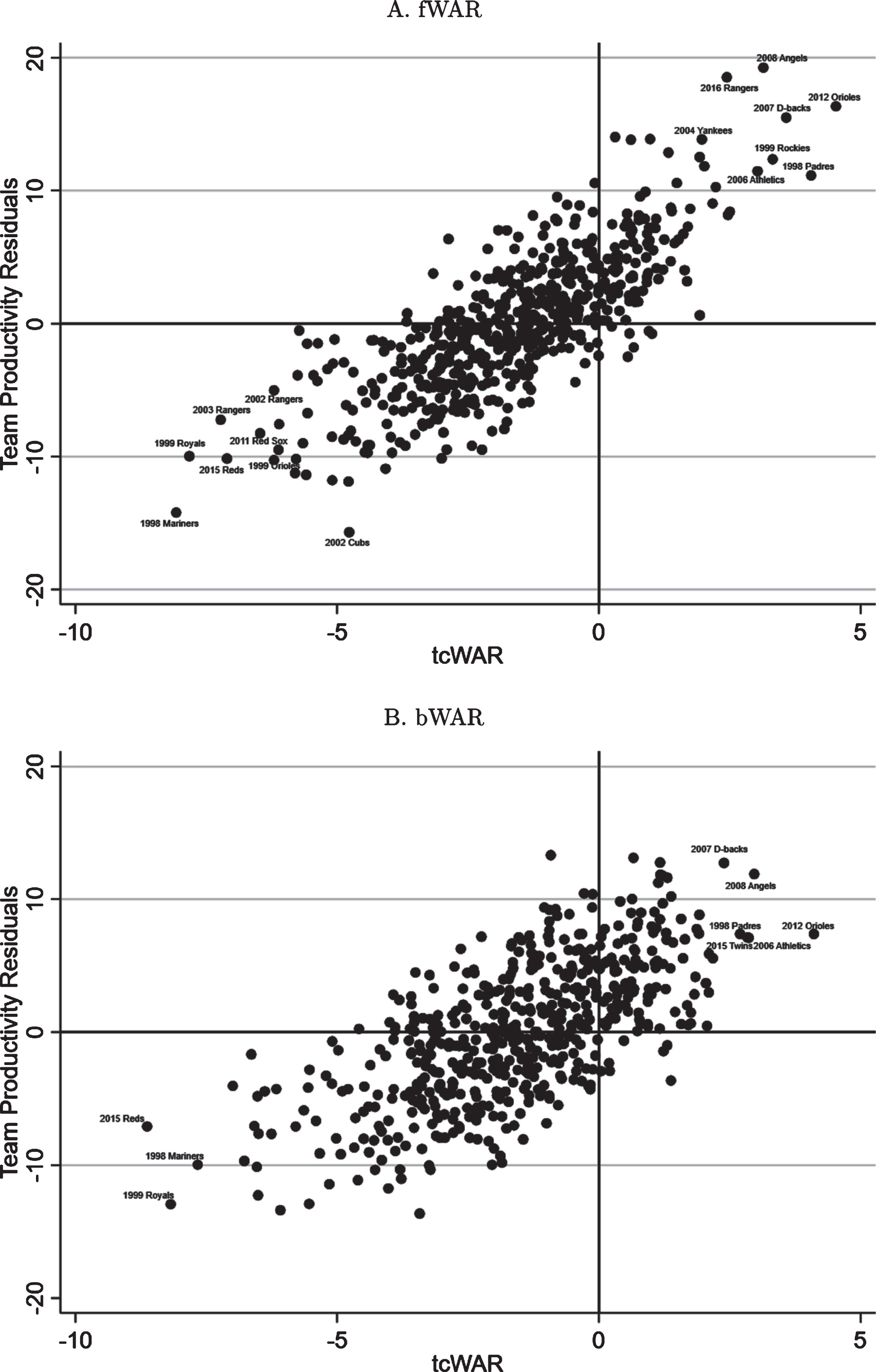
Figure 4 scatters a team’s productivity residual in each season against its tcWAR. The figure is constructed so that the x-axis coordinate (tcWAR) is equal to the number of team wins (y-axis coordinate) explained by team synergy. Some of the best and worst teams on both ends of the synergy spectrum are noted in the figure for both fWAR and bWAR results. While not identical, the teams that are singled out by both metrics on the basis of tcWAR overlap to a large degree. For instance, the 2012 Orioles, 2008 Angels, 2007 Diamondbacks, 2006 Athletics, and 1998 Padres all show up as teams with large positive tcWAR values and the 1998 Mariners, 1999 Royals, and 2015 Reds all show up as teams with large negative tcWAR values. While the size of the team productivity residuals tends to vary across fWAR and bWAR, the number of team wins that each metric attributes to team synergy remains fairly similar. For example, of the 2012 Orioles’ nearly 15 team wins above fWAR’s expectation, tcWAR attributes roughly 4 of these to good team synergy. In contrast, of the 2012 Orioles’ nearly 8 team wins above bWAR’s expectation, tcWAR attributes roughly the same number to team synergy.
Fig.4
Scatter plot of our team complementarity WAR (tcWAR) metric against our team productivity residuals for all MLB teams over the 1998-2016 seasons. Outlying team-season values referred to in the text are labeled for competing measures of wins-above-replacement (Fangraphs (fWAR) - panel A, Baseball-Reference (bWAR) - panel B).
Examining our tcWAR estimates on an organization-by-organization basis reveals that it is fairly rare for a team to over-achieve in terms of team synergy (tcWAR > 0); and, furthermore, those teams that do demonstrate very little persistence on this dimension. To confirm this, we regressed the current season’s tcWAR on the previous season’s value for the full panel of 30 MLB teams over the 1998-2016 seasons. These regressions for fWAR and bWAR data produced remarkably low estimates of first-order autocorrelation in team synergy; and, hence, exhibited very strong mean-reverting properties.1616 In this respect, our results are consistent with the notion that team synergy may be accurately described as “catching lightning in a bottle.” It is, therefore, likely to be an aspect of team performance that must be closely monitored and constantly managed by organizations.
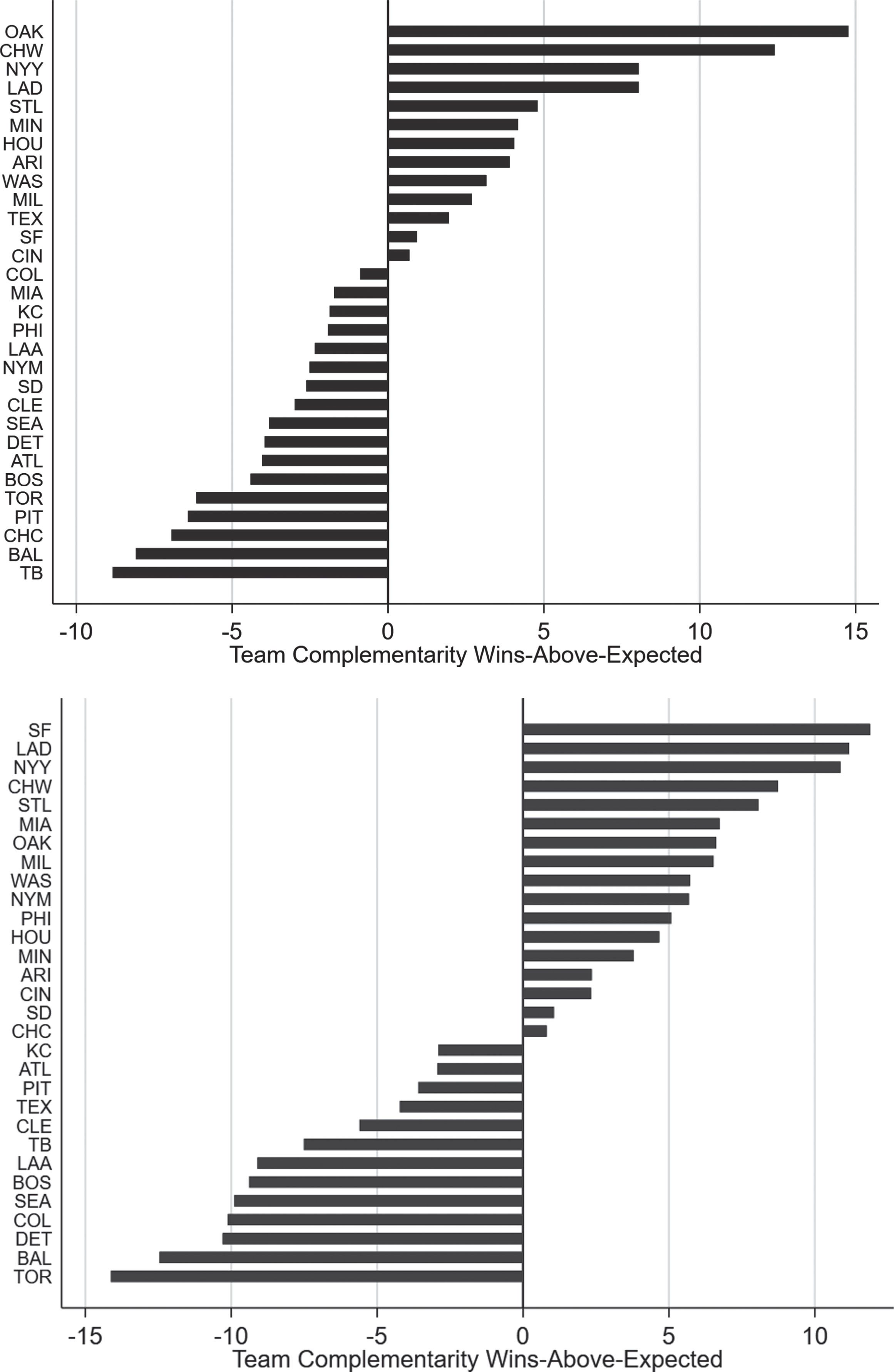
To identify organizations that have exceeded and fallen short of expectations on this dimension, we took the residuals from these regressions and summed them over time for each organization into a metric that we call “team synergy wins-above-expected.” Figure 5 presents the results of this exercise, ranking organizations from over- to under-achievers during our sample period. As with our Organizational Culture rankings, here, too, there exists some variability across fWAR and bWAR in interpreting team synergy. In some instances, the differences can be quite pronounced; as they are for the San Franciso Giants who top the bWAR rankings with nearly 10 wins above expected, but fall in the middle of the pack in the fWAR rankings with about 1 win above expected. A few organizations, however, stand out in both rankings, such as the Oakland A’s, Chicago White Sox, New York Yankees, Los Angeles Dodgers, and St. Louis Cardinals.
Fig.5
Cumulative team complementarity wins-above-expected for each MLB organization over the 1998-2016 seasons based on residuals from a regression of current season tcWAR on its previous season’s value. Panels of the figure display results for competing measures of wins-above-replacement (Fangraphs (fWAR) - panel A, Baseball-Reference (bWAR) - panel B).
The apparent lack of persistence in team synergy raises the question of what value tcWAR holds for a team or analyst. Therefore, to demonstrate its value we next show that the highly mean-reverting properties of team synergy are something that can be exploited to improve upon PECOTA’s pre-season team win projections. First, though, we consider the possibility that the information on team synergy found in tcWAR is already captured in PECOTA’s player-based projections. Table 3 contains the coefficients obtained by regressing PECOTA projections for the 2008-2016 seasons on the previous season’s projection, recursive estimates of the previous season’s tcWAR computed using only data through the previous season, and the combined previous season’s value of WAR for the current season’s roster. Interestingly, we find that at least part of what we measure in tcWAR does seem to be reflected in the PECOTA projections on either an fWAR or bWAR basis according to these regressions. This would seem to set a high bar then for tcWAR to provide any value-added over PECOTA. We show, however, that a very simple forecasting model incorporating the previous season’s team wins, the PECOTA projection, and a projected value of tcWAR based on the first-order autoregression described above can do just that.
Table 3
Team Win Projection Regressions: 2008-2016
| FanGraphs | Baseball-Reference | |||
| (1) PECOTAt | (2) Team Winst | (1) PECOTAt | (2) Team Winst | |
| PECOTAt - 1 | 0.537 | 0.560 | ||
| (0.071) | (0.069) | |||
| Team WARt-1 | 0.246 | 0.207 | ||
| (0.050) | (0.041) | |||
| tcWARt-1 | 0.260 | 0.374 | ||
| (0.123) | (0.114) | |||
| Team Winst - 1 | 0.363 | 0.315 | ||
| (0.076) | (0.073) | |||
| PECOTAt | 0.306 | 0.288 | ||
| (0.113) | (0.117) | |||
| Projected tcWARt | 16.653 | 13.554 | ||
| (2.245) | (1.619) | |||
| Constant | 29.140 | 54.450 | 28.772 | 53.024 |
| (4.360) | (5.528) | (4.391) | (5.818) | |
| R2 | 0.587 | 0.371 | 0.576 | 0.419 |
| MAE(PECOTA)–MAE(Model) | 1.251 | 1.487 | ||
| (0.426) | (0.505) | |||
| Observations | 240 | 270 | 240 | 270 |
Bootstrapped bias-corrected and accelerated standard errors clustered on team shown in parentheses based on 500 replications. Recursive estimates of tcWAR are used in specifications (1) and recursive one-step ahead projections in specifications (2). The mean absolute error (MAE) gain over PECOTA is based on a Diebold-Mariano test of equal MAE using 240 out-of-sample predictions of team wins.
To see why this is the case, Table 3 also contains the results for these regressions using the full sample of data. Even after accounting for the PECOTA projection, the regressions calculated on either an fWAR or bWAR basis still load significantly onto tcWAR, suggesting there is information in our metric that is not captured by the PECOTA forecast. Using out-of-sample one-step ahead projections from this regression, we find that it would have been possible to improve upon PECOTA pre-season projections by a statistically significant margin of roughly 1 win based on a Diebold and Mariano (1995) test of equal mean absolute error across models. While the magnitude of this improvement may seem small, for our purposes it is sufficient to demonstrate that tcWAR contains information that is not already summarized in PECOTA. We leave it to future work to determine whether or not this result can be improved upon, perhaps through a reconfiguration of PECOTA’s projection system to also account for the player complementarity effects that we discuss next.
4.3Player evaluation
We can also refine WAR as a measure of player performance by taking into account how much a player affects his teammates’ performances. Here, we add to WAR- the contribution of each player to all of his teammates’ productivity residuals, or what is referred to in network statistics as the “out-degree” of a node. We call this measure WAR+.
(14)
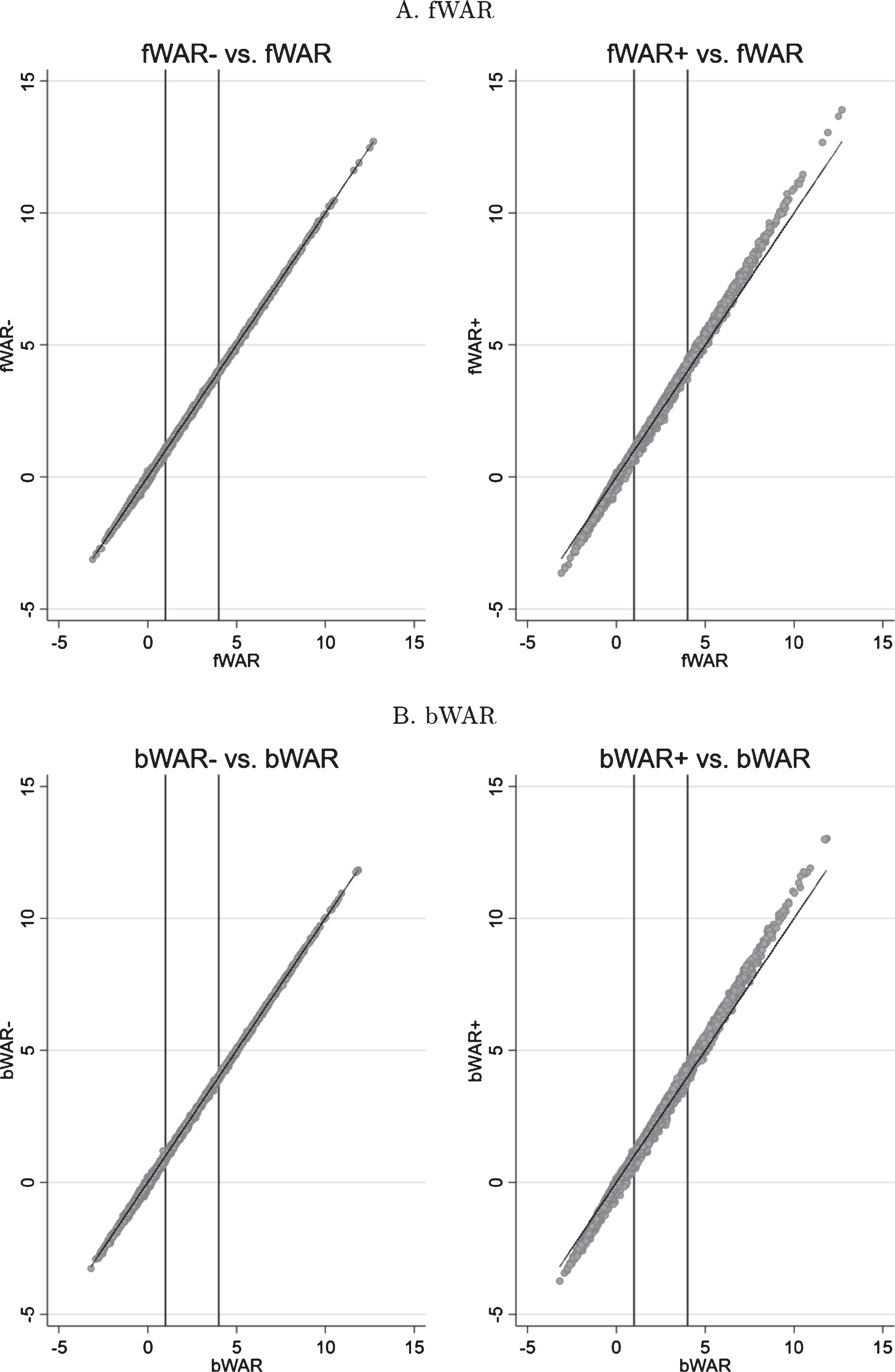
Figure 6 scatters WAR- and WAR+ versus WAR on an fWAR and bWAR basis. Interestingly, WAR- and WAR on an individual player-season basis are very highly correlated, with the plotted points clustered fairly closely around the 45 degree line. Thus, it is the aggregation of somewhat small differences at the player level that leads to the drastic reduction in the unexplained variance of team performance in Table 1 and Fig. 2. For WAR+, on the other hand, the differences are much more pronounced. In particular, our analysis suggests that WAR overestimates the relative performance of low impact (WAR < 1), and underestimates the relative performance of high impact (WAR > 4) players on team performance.1717
Fig.6
Scatter plot of competing measures of wins-above-replacement (Fangraphs (fWAR) - panel A, Baseball-Reference (bWAR - panel B) against our WAR- and WAR+ metrics for MLB players spanning the 1998-2016 seasons. Solid lines in each graph correspond with 45 degree lines, while the vertical lines denote threshold values from Fangraphs for Scrub/Role (WAR = 1) and Good/Star (fWAR = 4) players.
The difference between WAR+ and WAR can be used to evaluate players on the basis of their contribution to team performance through their impact on their teammates. In network statistics, this is what is called the “net-degree” for each node.
(15)
In keeping with our terminology above, we instead refer to it as “player complementarity wins-above-replacement,” or pcWAR. In Fig. 7, we plot the pcWAR for all player-season combinations in our dataset relative to a player’s WAR on an fWAR and bWAR basis. Notice that summing a player’s pcWAR and WAR reproduces our WAR+ metric, such that adding the x-axis and y-axis coordinates for each player-season in this figure provides a sense of his true value to his team.
Fig.7
Scatter plot of competing measures of wins-above-replacement (Fangraphs (fWAR) - panel A, Baseball-Reference (bWAR) - panel B) against our player complementarity WAR (pcWAR) metric for MLB players spanning the 1998-2016 seasons. Vertical lines denote threshold values from Fangraphs for Scrub/Role (WAR = 1) and Good/Star (WAR = 4) players.
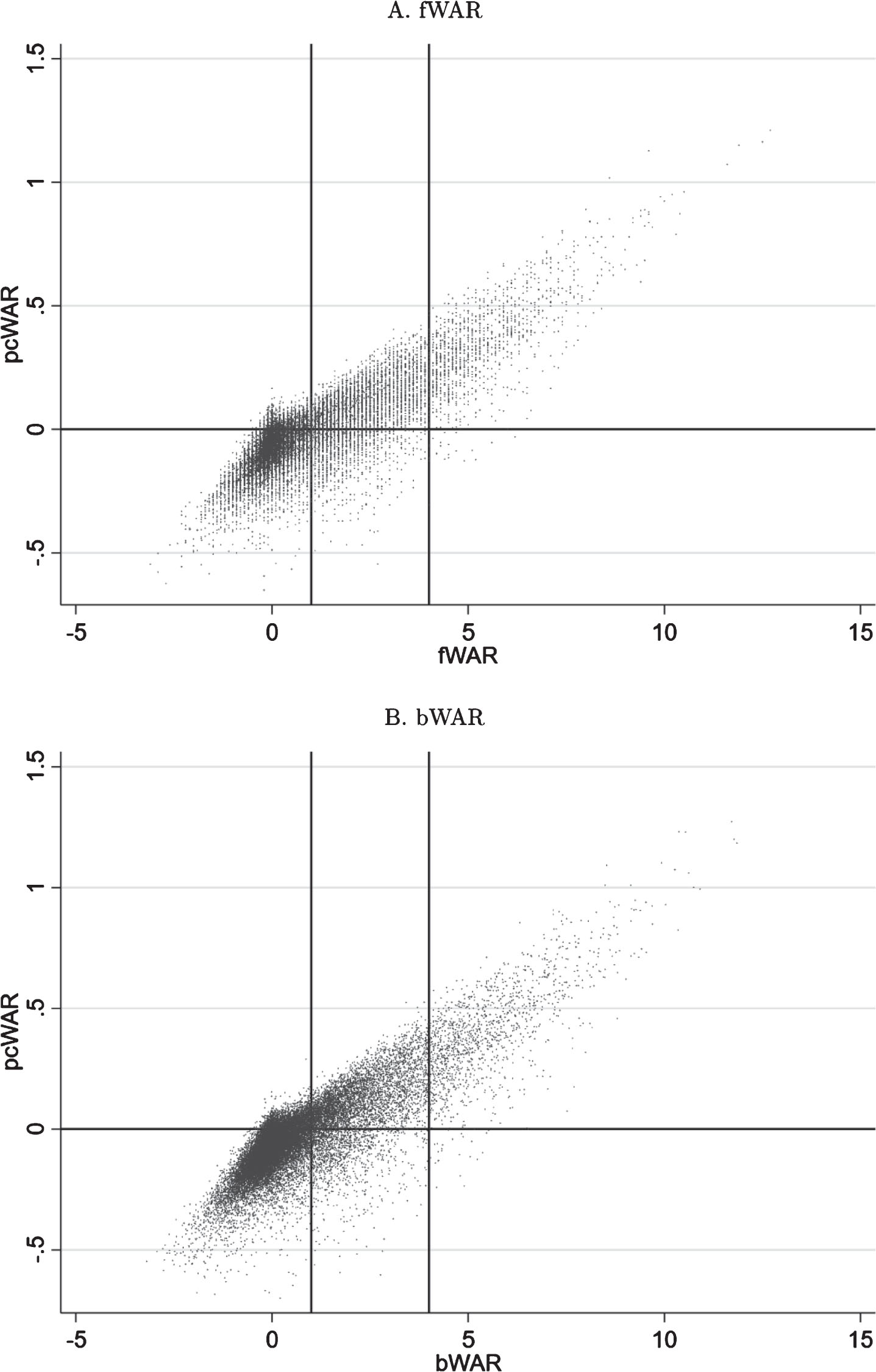
The conventional wisdom that good players make their teammates better is confirmed by our analysis of pcWAR, as Fig. 7 demonstrates a strong positive correlation exists between pcWAR and WAR for all player-season combinations in our sample. The vertical lines in the figure correspond to thresholds for WAR used by FanGraphs to distinguish Good from Star players (WAR = 4) and Scrub from Role players (WAR = 1). Star players tend to add anywhere from about 0 to 1.5 wins to their team through their indirect impact on the performance of their teammates, whereas Scrub players tend to add from about 0 to 0.5 losses to their team. In between, there exists considerable variation with players contributing from -0.5 to 0.5 wins.
The impact of Star players on their teammates likely comes through so strongly in our analysis because they are among the most talented; and, therefore, have skill sets that are just naturally likely to be more complementary to others on the team in a variety of ways. We show below, however, that even still there exists a considerable amount of diversity across these players in how much this is the case. Part of the reason for this likely reflects the team-related aspects of complementarity, i.e. the player is just a bad fit for the team as a whole, but part also boils down to the player’s ability (or willingness) to adapt to his teammates.
Figure 8 ranks all active players through the 2016 season on the basis of their career average pcWAR values.1818 The left-hand panel of the figure shows the top 25% of players on this dimension, while the right-hand panel shows the bottom 25%. Many of the top players in the game dominate our leaderboard, with Mike Trout the undisputed champion in this regard, averaging over one-half win of additional value over the course of his career. While our estimates for pcWAR may seem small at first glance in terms of win value, they are of a non-trivial economic value. With a team win valued at roughly $6 million in MLB, the value of team synergy alone for some of the game’s best players is just as high according to our pcWAR metric as what WAR would assign to a typical role player on the team (Cameron, 2014). In fact, even a player whose WAR was 0 and pcWAR was as low as 0.1 would still be worth paying the MLB minimum salary.
Fig.8
Ranking of active MLB players through the 2016 season on their career average pcWAR values broken down into contributions from player- and team-specific components and constructed from competing measures of wins-above-replacement (Fangraphs (fWAR) - panel A, Baseball-Reference (bWAR - panel B). Left-hand side of each panel displays the top 25% of rankings, while the right-hand side shows the bottom 25% of rankings.
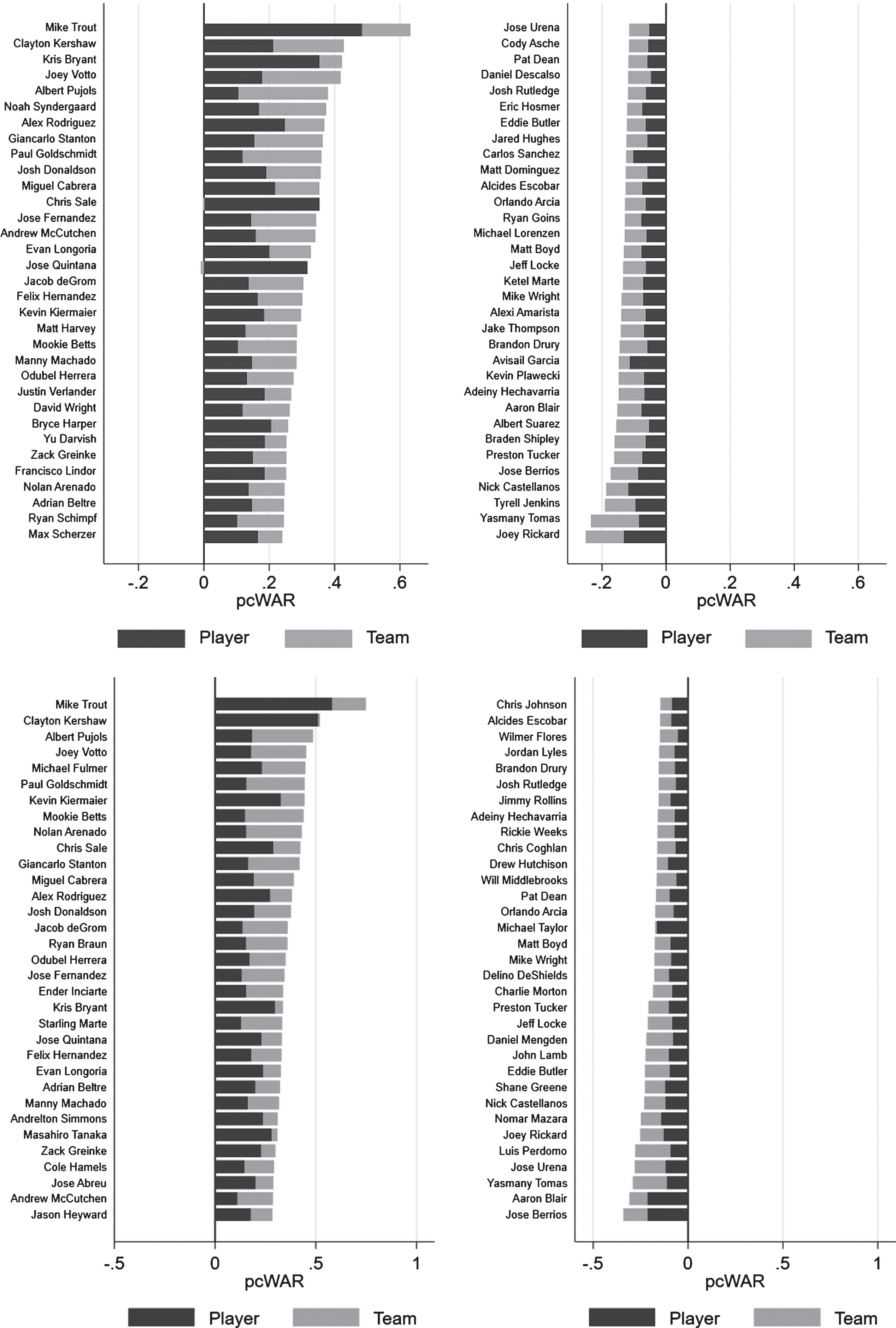
The figure also breaks down pcWAR into separate components due solely to characteristics of the player (e.g. the contributions from the “character” factor of our model) versus other contextual factors related to the team (e.g. the contributions from the “team player” factor of our model). The former component of pcWAR is potentially of value for teams looking to alter their synergy profile through trades or free agency, as it strips out any previous organizational effects. For example, a common criticism of general managers of the consideration of leadership qualities in the evaluation of another team’s player is that it is difficult to ascertain how much of a player’s past performance is the result of his previous team environment versus some innate ability (Olney, 2018). Our method allows for a disentangling of such effects.
At the player level, team synergy is also much more persistent, with pcWAR lending itself more easily to prediction than tcWAR. This can be seen in Table 4 in the coefficients of the regressions of the current season’s pcWAR on the talent level of the player (e.g. Star, Role, Scrub) based on his previous season’s WAR and its interaction with the previous season’s pcWAR value. The persistence of a player’s complementarity effects is increasing in past performance, with Star players exhibiting nearly five times the persistence as Scrub players and about 1.5 times as much as Role players. This suggests that player complementarity expectations based on past performance may be an appropriate guide for teams to judge their own players.
Table 4
pcWAR Regressions
| FanGraphs | Baseball-Reference | |||
| (1) pcWARt | (2) pcWARt | (1) pcWARt | (2) pcWARt | |
| pcWARt-1 * (WARt-1 < 1) | 0.128 | 0.044 | 0.104 | 0.045 |
| (0.015) | (0.008) | (0.013) | (0.007) | |
| pcWARt-1 * (1 ≤ WARt-1 < 4) | 0.375 | 0.168 | 0.302 | 0.161 |
| (0.022) | (0.013) | (0.024) | (0.013) | |
| pcWARt-1 * (WARt-1 ≥ 4) | 0.576 | 0.244 | 0.521 | 0.211 |
| (0.041) | (0.019) | (0.046) | (0.020) | |
| WARt-1 < 1 | –0.043 | –0.043 | ||
| (0.001) | (0.002) | |||
| 1 ≤ WARt-1 < 4 | –0.020 | –0.037 | –0.029 | –0.046 |
| (0.002) | (0.002) | (0.003) | (0.002) | |
| WARt-1 ≥ 4 | –0.039 | –0.117 | –0.049 | –0.133 |
| (0.014) | (0.008) | (0.018) | (0.009) | |
| WARt | 0.094 | 0.108 | ||
| (0.001)) | (0.001) | |||
| MLB Experiencet | -5.67e-5 | -7.16e-5 | ||
| (4.13e-6) | (4.11e-6) | |||
| Team Experiencet | -5.79e-5 | -7.18e-5 | ||
| (5.98e-6) | (7.26e-6) | |||
| League Fixed Effects | X | X | ||
| Team Fixed Effects | X | X | ||
| Manager Fixed Effects | X | X | ||
| Age-Position Interactions | X | X | ||
| R2 | 0.214 | 0.795 | 0.147 | 0.815 |
| Players | 4,112 | 4,112 | 4,112 | 4,112 |
| Observations | 20,735 | 20,735 | 20,735 | 20,735 |
Bootstrapped bias-corrected and accelerated standard errors clustered on player shown in parentheses based on 500 replications. Age-Position interactions include up to quartic terms in age. WARt-1 < 1 coefficient is absorbed in the position indicators to prevent multicollinearity in specifications (2).
Just as we did with teams, we can use these regressions to define “player complementarity wins-above-expected” by taking their residuals and summing them over a player’s career. Figure 9 plots the resulting measure against each player’s average of his previous seasons’ WAR values. The vertical lines in the figure correspond to the FanGraphs thresholds, while the horizontal lines are used to highlight the extremes of the distribution. Each dot in the figure then represents a player’s career complementarity wins-above-expected, with notable examples highlighted in order to identify players in our sample who have exceeded or fallen short of expectations on this dimension.
Fig.9
Scatter plot of individual players’ career complementarity wins-above-expected against the average of his previous season’s wins-above-replacement over the 1998-2016 seasons for competing measures (Fangraphs (fWAR) - panel A, Baseball-Reference (bWAR) - panel B). Vertical lines denote threshold values from Fangraphs for Scrub/Role (WAR = 1) and Good/Star (WAR = 4) players, with outlying player values referred to in the text labeled in each panel.
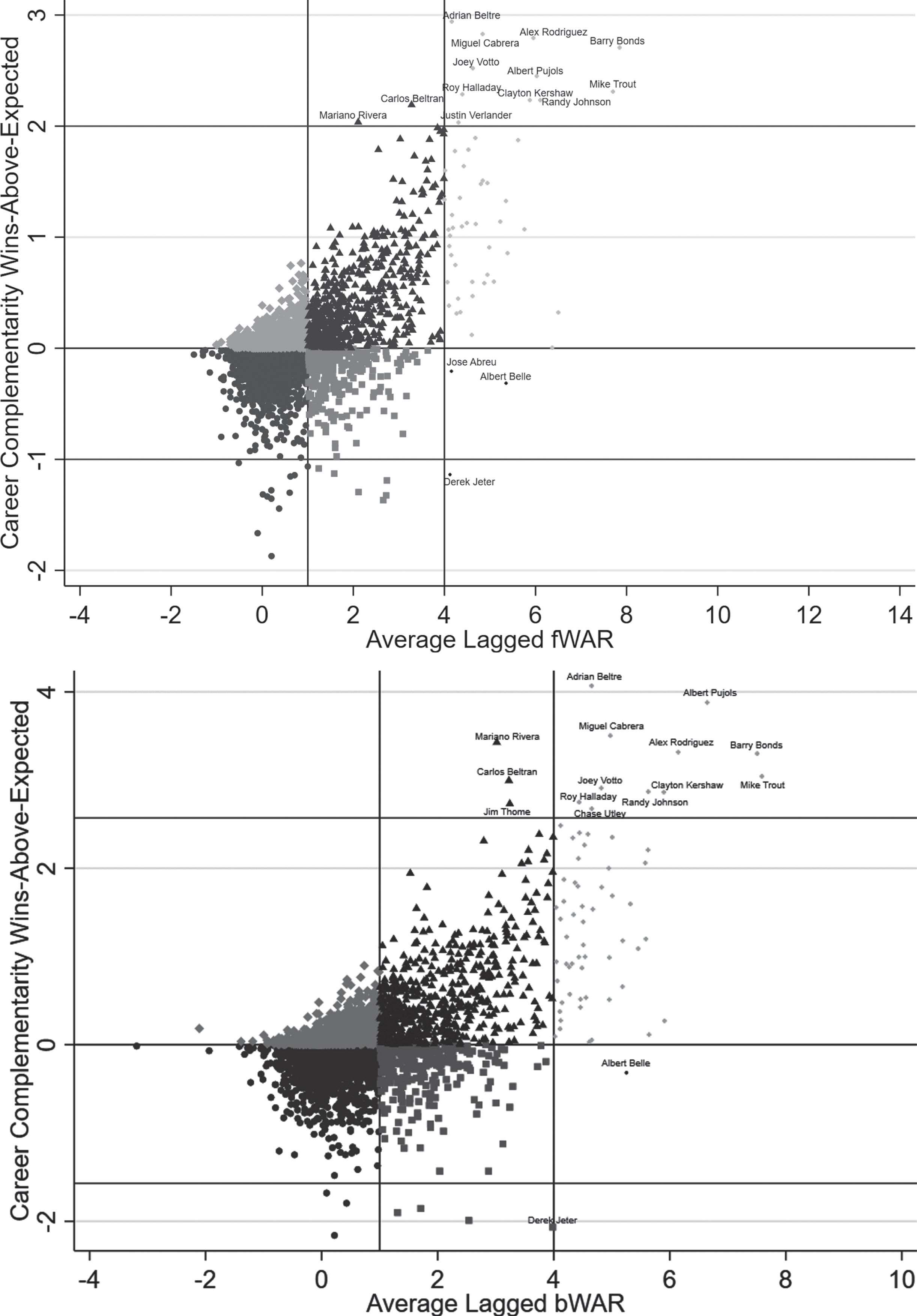
The good players make their teammates better paradigm is also highly evident in this figure, but the proximity (or lack thereof) between certain players also draws out some interesting comparisons. For instance, the early career of Clayton Kershaw and late career of Randy Johnson look very similar on this dimension whether they are measured on an fWAR or bWAR basis. In contrast, Derek Jeter represents an extreme outlier in this analysis for a Star player with a career complementarity wins-above-expected that is both negative and from four to six wins less than Adrian Beltre, the career leader during our sample period. There are also a handful of Role players according to WAR with career complementarity wins-above-expected on par with the top 10 Star players in our sample (e.g. Mariano Rivera, Carlos Beltran, and Jim Thome), and a handful of Star players that show negative career complementarity wins-above-expected (e.g. Jose Abreu, Albert Belle, and Derek Jeter) on an fWAR or bWAR basis.
5Complementarity and roster construction
Our aim in this section is to develop some additional convenient “rules-of-thumb” for MLB general managers to follow when considering team synergy in roster construction. We first explore the drivers of player complementarity by constructing age-position profiles for pcWAR conditional on player and team characteristics. These profiles then allow us to rank players on the dimension of their unobserved Intangibles. Because salary negotiation plays such an important role in roster construction, this leads naturally then to a discussion of the value of the observed and unobserved aspects of player complementarity.
5.1Age-position profiles and intangibles
We construct our conditional average age-position profiles for player complementarity by extending the pcWAR dynamic regressions discussed above according to,
(16)
where pos is an indicator variable for a player’s primary defensive position, including the designated hitter and a “utility” category for players who tend to play multiple defensive positions, age is a player’s age, X is a vector of player characteristics including WAR and controls for MLB and team games played, and Z is a vector of league, team, and manager indicator variables. The estimated coefficients of these regressions are summarized in Table 4.
Figure 10 plots our conditional average age-position pcWAR profiles with 95% confidence intervals on an fWAR and bWAR basis. The conventional wisdom that older players make for better teammates is certainly consistent with these profiles, as they tend to slope upward with age on average across almost all positions. However, we want to caution anyone from taking the results from this regression as “causal” estimates of age on team synergy, as the estimated coefficient is most likely also confounding a selection effect. In other words, having good team synergy may make it more likely for a player to remain in the game for longer.
Fig.10
Age-position player complementarity profiles based on our pcWAR metric as constructed from competing measures of wins-above-replacement (Fangraphs (fWAR) - panel A, Baseball-Reference (bWAR) - panel B). Bootstrapped bias-corrected and accelerated 95% confidence intervals clustered on player observations are shown in gray, with solid lines corresponding to average marginal effects over ages from 20-40 for each position.
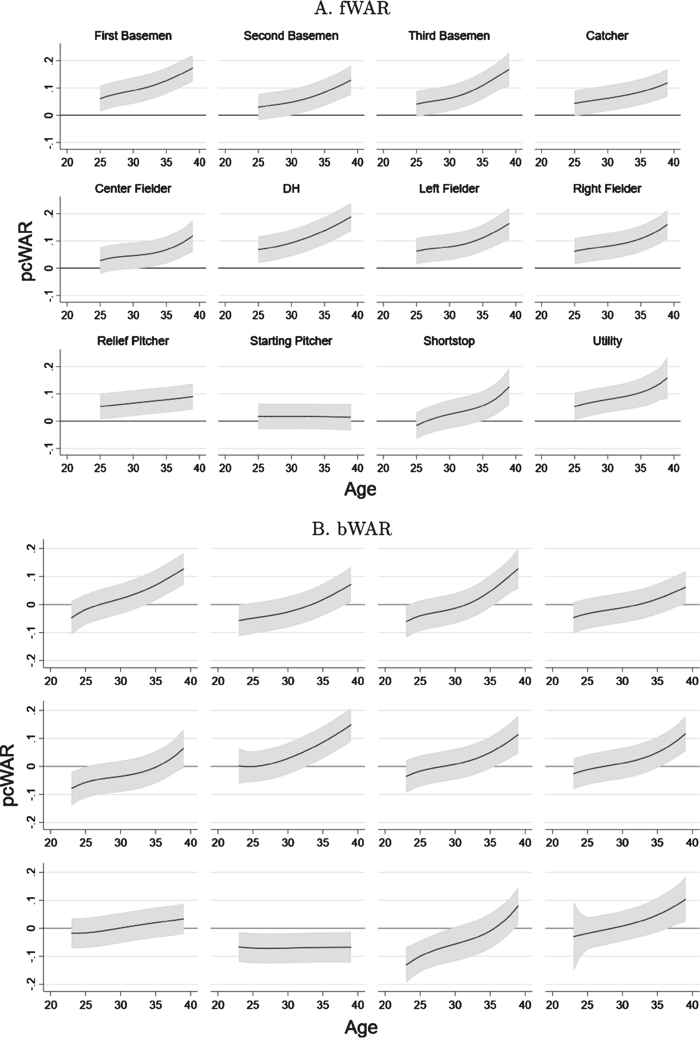
Some additional interesting patterns also emerge from this analysis. For instance, the slopes of these profiles tend to vary by position. Second basemen and catchers tend to have profiles that are less steep than other infielders; relief pitchers tend to have steeper profiles than starting pitchers; and the profiles of designated hitters and utility players tend to be among the steepest that we estimate. The level of the profiles also varies depending on whether or not they were constructed on an fWAR or bWAR basis, with complementarity effects generally more positive across all positions and ages when measured on theformer.
By conditioning these regressions on so many observable dimensions, we can also isolate the player Intangibles of team synergy. In other words, we can measure the individual contributions to team wins through player complementarities that are not associated with any covariates in the above regressions. We use the residuals, ξit, from these regressions to rank active players through the 2016 season on their career average Intangibles. Positive residuals capture players whose contributions to team synergy exceed their conditional age-position profile, whereas negative residuals correspond to players who fall short of their profile.
Figure 11 displays our Intangibles rankings, where the left-hand panel shows the top 25% of players on this dimension and the right-hand panel shows the bottom 25%.1919 Our top players are now very different than who they were for pcWAR, with the exception of Joey Votto who shows up in the top four of both rankings. Kevin Keirmaier is the undisputed active leader on this dimension of team synergy, with an average contribution of a little more than 0.1 wins coming from his Intangibles.
Fig.11
Ranking of active MLB players through the 2016 season on their career average Intangibles values constructed from competing measures of wins-above-replacement (Fangraphs (fWAR) - panel A, Baseball-Reference (bWAR - panel B). Left-hand side of each panel displays the top 25% of rankings, while the right-hand side shows the bottom 25% of rankings.
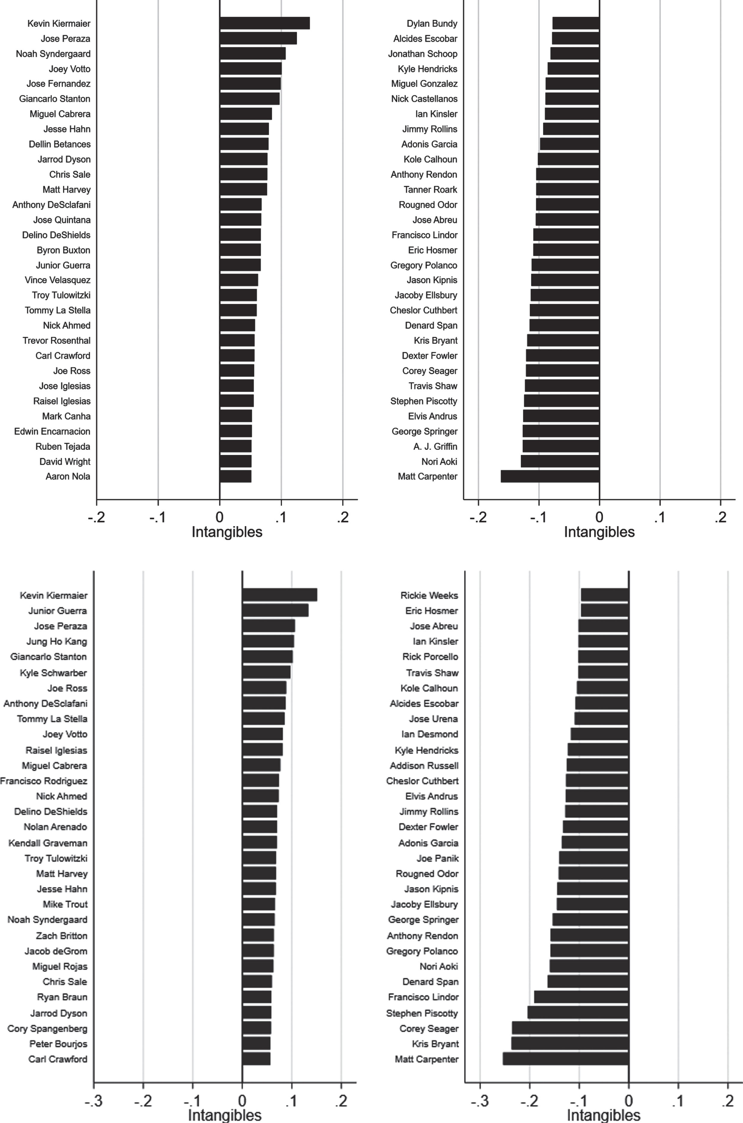
At this point, a word of caution is warranted. Many of the players who we find have negative Intangibles are the same type of player that any MLB franchise would be happy to build their team around. In other words, depending on a player’s position, his age, and current manager, etc., he could still have a strong positive influence on his teammates even despite a negative Intangibles measure. A more appropriate interpretation of the rankings in Fig. 11 is then that they provide an indication of those players who have a knack for exceeding expectations on the dimension of team synergy. We call this the “David RossEffect.”
The esteem with which the 2016 World Champion Chicago Cubs held their teammate David Ross and his contribution to their success has by now become well known. The ability of a team to identify players like him is, therefore, a potential source of competitive advantage that is made possible by our player complementarity metrics. What makes David Ross uniquely suited to our analysis is that, as a back-up catcher, his WAR defines him as a role player; but, as a teammate, he is routinely characterized as someone who makes everyone around him better. We are able to provide evidence to support these claims with our metrics.
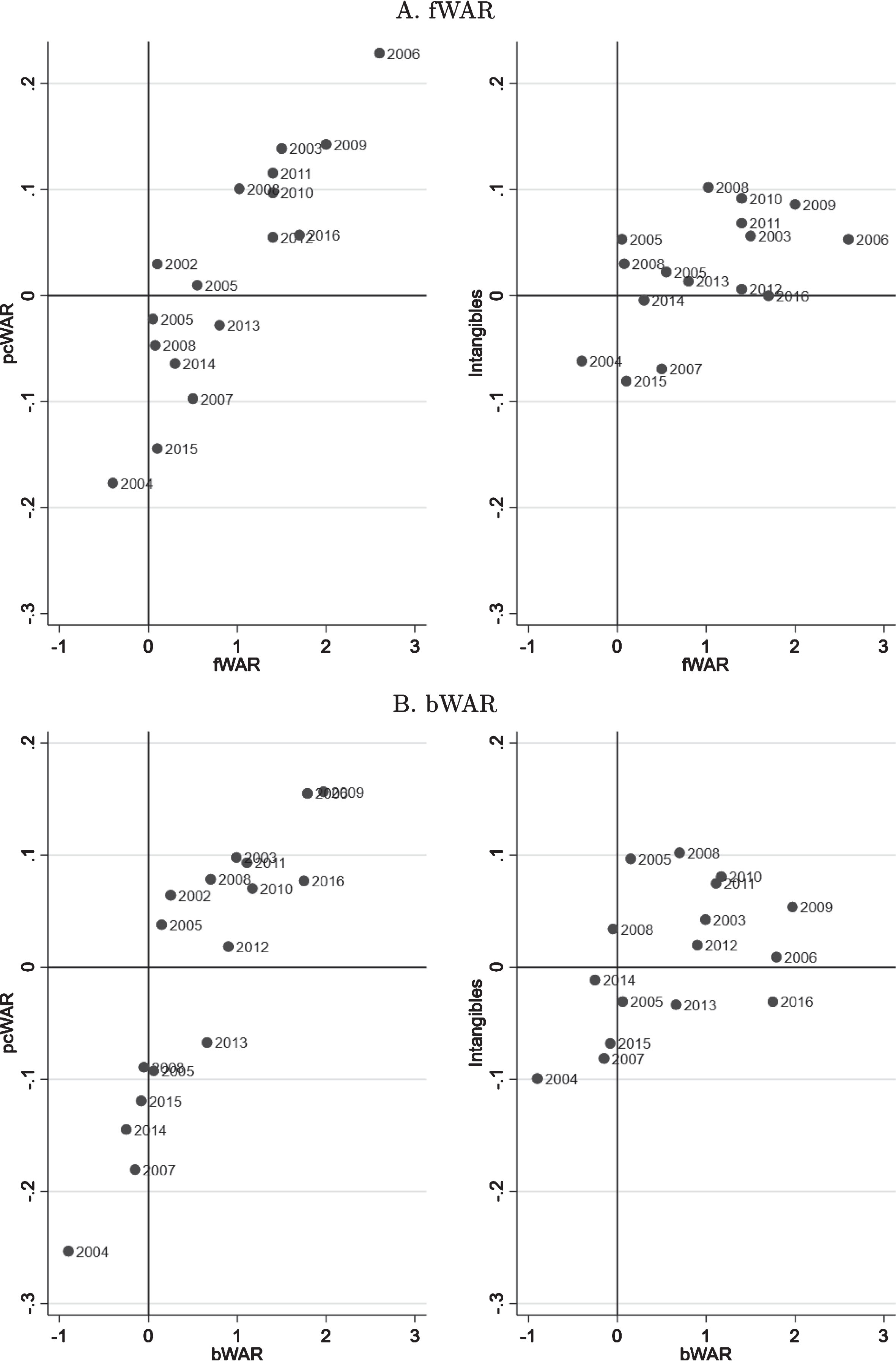
Figure 12 plots the pcWAR and Intangibles values for David Ross through the 2016 season against his WAR values. More than one labeled instance of a season occurs whenever he was traded. For most of his career, and across several different teams, David Ross exhibited the sort of beneficial relationship with his teammates that his reputation attests to, evidenced by his mostly positive pcWAR values. Furthermore, his Intangibles reveal a player who tended to outperform his age-position profile even at low levels of WAR and with limited playing time.
Fig.12
Scatter plot of pcWAR values against competing measures of wins-above-replacement (Fangraphs (fWAR) - panel A, Baseball-Reference (bWAR - panel B) for David Ross in each season of his career. More than one value appears for seasons where David Ross was traded to another team in-season.
Players such as David Ross are true “diamonds-in-the-rough” according to our analysis, with their full impact on team performance likely to fly under the radar according to traditional performance metrics. Given how rare that we find that this type of player is in our analysis, one might expect that MLB teams would be willing to pay a premium for their services. For example, others have already documented the importance of wins-above-replacement in pricing player services in MLB.2020 For this reason, we might expect our pcWAR metric to also be priced into player compensation. Whether or not this extends to a player’s Intangibles, which are much more difficult to observe than age, position, and the other variables that we condition on, is unclear.
5.2Putting a price on complementarity
To see how MLB teams have historically valued player complementarity, we run player-level regressions of log annual salary adjusted for inflation (using the U.S. Consumer Price Index) as our dependent variable on a player’s career WAR and pcWAR through the previous season.2121 This regression takes the following form,
(17)
where pos is an indicator variable for a players’ primary defensive position, including the designated hitter and a “utility” category for players who tend to play multiple defensive positions; age is a player’s age on January 1st of the year in which season t occurs; teamExp indicates the number of seasons the player has appeared in with his current team prior to the current season; mlbExp is the number of MLB games in which the player has appeared through the previous season; FA is an indicator variable which takes on one of three values denoting whether a player is in the pre-arbitration (0–2 years of service), arbitration-eligible (3–5 years), or free agent-eligible (6+ years) stage of his career; and αi is a player fixed effect.
The use of a player fixed effect focuses our analysis on the variation “within” player salary histories. For this reason, we restrict our sample of players to only those with careers that began at some point during the 1998-2016 seasons. As we will soon explain, the inclusion of the FA indicator variable serves to capture important differences in how player salaries are determined throughout a career based on the labor market structure of MLB and changes in the bargaining power of players according to service time.2222 We interact this variable with teamExp to then capture the impacts of trades and other reasons for team changes on service time and player salaries. The inclusion of pos and its interaction with age and experience then serves to capture any nonlinear variation in how players’ career earnings trajectories vary across defensive positions.
We are primarily interested in obtaining estimates for γ and β, the coefficients on career WAR and pcWAR, respectively. Interacting these variables with our service time-status indicator allows us to estimate how these skills may be differentially priced over a player’s career. As the first column of Table 5 shows, cumulative WAR is indeed priced differentially throughout a player’s career. During the pre-arbitration stage of a player’s career, a one win-above-replacement increase in career WAR through the previous season leads, on average, to a statistically significant earnings increase in the current season of 10-12 percent. For a player in the arbitration-eligible portion of his career, this increases slightly to 14 percent. Finally, players with six or more years of MLB service time see an average increase in earnings of 4-5 percent for each additional unit of career wins-above-replacement.
Table 5
Player Salary Regressions
| FanGraphs | Baseball-Reference | ||||
| (1) log(Salary) | (2) log(Salary) | (1) log(Salary) | (2) log(Salary) | ||
| FA0*Career WAR | 0.10*** | 0.09*** | 0.12*** | 0.10*** | |
| (0.02) | (0.01) | (0.02) | (0.01) | ||
| FA1*Career WAR | 0.14*** | 0.13*** | 0.14*** | 0.13*** | |
| (0.01) | (0.01) | (0.01) | (0.01) | ||
| FA2*Career WAR | 0.04*** | 0.02** | 0.05*** | 0.02*** | |
| (0.01) | (0.01) | (0.01) | (0.01) | ||
| FA0*Career pcWAR | -0.20 | -0.31** | |||
| (0.16) | (0.14) | ||||
| FA1*Career pcWAR | -0.50*** | -0.54*** | |||
| (0.06) | (0.05) | ||||
| FA2*Career pcWAR | 0.12** | 0.01 | |||
| (0.06) | (0.05) | ||||
| FA1*Career (pcWAR - ξ) | -0.46*** | -0.44*** | |||
| (0.07) | (0.07) | ||||
| FA2*Career (pcWAR - ξ) | 0.47*** | 0.31*** | |||
| (0.07) | (0.06) | ||||
| FA1*Career ξ | -0.31*** | -0.38*** | |||
| (0.09) | (0.08) | ||||
| FA2*Career ξ | -0.35*** | -0.37*** | |||
| (0.08) | (0.07) | ||||
| Contract Status Indicator (FA) | X | X | X | X | |
| FA-Team Experience Interactions | X | X | X | X | |
| Position Indicator | X | X | X | X | |
| Age-Position Interactions | X | X | X | X | |
| Position-MLB Experience Interactions | X | X | X | X | |
| Position-MLB Experience2 Interactions | X | X | X | X | |
| Player Fixed Effects | X | X | X | X | |
| R2 | 0.86 | 0.86 | 0.86 | 0.86 | |
| Players | 4,117 | 4,117 | 4,117 | 4,117 | |
| Observations | 18,114 | 18,114 | 18,114 | 18,114 | |
*** p<0.01, ** p<0.05, * p<0.1 Select variable estimates reported. Specifications include a contract status indicator (FA) and its interaction with years with current team along with a position indicator and its interactions with age, games of MLB experience, and experience squared in addition to player fixed effects. FA0 interactions with pcWAR - ξ and ξ are absorbed to prevent multicollinearity in specifications (2). Bootstrapped bias-corrected and accelerated standard errors clustered on player shown in parentheses based on 500 replications.
To understand the pricing pattern demonstrated in this result, it is useful to consider the bargaining position of the player. The pre-arbitration period corresponds to a player’s first three years of service time, measured by days spent on the 25-man roster of any MLB team. Unless released or traded, players are bound to the team that drafted them during this period. The vast majority of these players earn either a minimum salary determined by collective bargaining between MLB and the MLB Players Association or a somewhat higher salary on a season-by-season basis that is at the discretion of the team. Performance and salary are, therefore, likely to be only somewhat correlated during this time. Furthermore, even if a player were to sign a long-term contract during this time, they lack the bargaining power they would have if their services were being priced by the entire league, an economic situation referred to as monopsony.
If a player still has not signed a long-term contract after three years of service, they become eligible for salary arbitration, whereby the player and team submit proposed salaries to an independent third party that makes a binding determination on the player’s salary, largely on the basis of similar player performances.2323 Though players still have limited bargaining power during this period, the slight increase in the return to cumulative WAR that we observe is consistent with their improved bargaining position afforded by the arbitration process. When a player has not signed a long-term contract after accruing six or more years of MLB service time, he becomes eligible to sign with any team as a free agent.
Once a player enters free agency, it is much more common for him to sign a multi-year contract. Multi-year contracts add a further complication to our regression, since their pricing reflects a weighted combination of both past and expected future performances. This could largely explain the smaller coefficient that we find on cumulative fWAR during free agency. However, the competitive landscape of free agency may also force teams to consider a broader range of factors as they submit contract offers to players. In fact, our estimated regression coefficients on cumulative pcWAR suggest that a player’s complementary skills are perhaps one of the additional things considered.
The specifications marked (1) in Table 5 show that cumulative pcWAR is also priced differentially throughout a player’s career. The effect on earnings of a one win-above replacement increase in career pcWAR is large, negative, and statistically significant (with the exception of pre-arbitration players on a bWAR basis) in the pre-arbitration and arbitration-eligible periods. This suggests that the lack of competitive pressure in these years allows teams to avoid compensating players for their complementary skills. However, this effect reverses once a player becomes eligible for free agency, as the same increase in pcWAR now leads to a small salary gain that is only statistically significant on an fWAR basis.
It may seem counterintuitive that the marginal return to a unit increase in cumulative pcWAR is roughly on par or higher than that for a unit increase in cumulative WAR during free agency. However, as a relatively scarce resource (its standard deviation is nearly 15 times smaller than cumulative fWAR or bWAR), it makes sense that cumulative pcWAR is priced as such on the margin. That said, it could also just as easily be the case that what we find reflects a team’s pricing of some of pcWAR’s underlying correlates. For instance, if MLB teams follow the conventional wisdom that high-performing players will have the biggest synergy effects, they may simply pay more for individuals who they expect will rank highly in the future on metrics such as fWAR and bWAR. The coefficient on cumulative pcWAR would then reflect this fact.
To investigate this possibility, we run an alternative earnings regression that instead considers separately our Intangibles measure (i.e. ξ) and the observed component of pcWAR (i.e. pcWAR - ξ). These results, marked as specifications (2) in Table 5, show that the two individual components of cumulative pcWAR are indeed priced differently in free agency (i.e. their coefficients have opposite signs) and in a similar fashion across fWAR and bWAR. A player with positive career Intangibles would be undervalued relative to his contribution to the team; and, conversely a player with negative career Intangibles would be overvalued. In contrast, the observed component of cumulative pcWAR for either player would still be appropriately valued. This result suggests an important application for our metrics. Though teams appear to value their players’ complementary skills, they clearly “misprice” their Intangibles. This is most likely because they are not easily observed and, therefore, difficult to evaluate in an efficient enough manner in which to price them.
6Conclusion
In this paper, we outlined a methodology for quantifying how a player may influence his team’s performance outside of his direct contribution measured by advanced individual performance metrics like wins-above-replacement. We introduced in the process WAR-, WAR+, tcWAR, and pcWAR as new advanced metrics that quantify a team’s synergy, or the indirect effects of players on their teammates and team performance, while providing an intuitive analog to FanGraph’s and Baseball-Reference’s well-documented fWAR and bWAR metrics. With these new metrics, we then outlined the importance of accounting for player interactions in explaining team performance differentials unexplained by WAR.
With tcWAR, we further demonstrated that team synergy is difficult to preserve, making it an aspect of team performance that must be closely monitored and constantly managed. We also examined the organizational aspects of team synergy, ranking organizations on their ability to reinforce positive or minimize negative interactions between teammates, as well as preserve team synergy over time. Furthermore, we showed how tcWAR’s mean-reverting properties could be used to improve upon PECOTA pre-season projections of team wins.
At the player level, we found more persistence in the aspects of player complementarity that contribute to team synergy, particularly for star players, and we documented how pcWAR could be used to guide team decision-making for its own players and in trades and free agency by separating out the player-specific and team-related elements of synergy. We also developed convenient “rules-of-thumb” for general managers to follow when considering team synergy in roster construction, demonstrating that star and older players tend to make for good teammates and that the rate of development of players’ complementary skills varies by position.
By conditioning on a large set of observable team and player characteristics, we were also able to isolate a player’s Intangibles, defined by whether or not their pcWAR value exceeds or falls short of these characteristics. This allowed us to quantify what we call the “David Ross Effect,” so named after the back-up catcher who consistently outperformed his observable characteristics for much of his career. Furthermore, we demonstrated that MLB teams have in the past placed too low of a value on the Intangibles aspect of team synergy than the value of a win would suggest is appropriate.
These results paint a clear picture of the role of team synergy in MLB. Despite having a large influence on team outcomes, our analysis suggests that most of the predictable component of this factor year-to-year is concentrated in the star players that are already heavily sought after in the free agent market. Alternatively, the players whose intangibles are likely to be underpriced are also those whose intangibles are also less likely to be persistent from year-to-year. Given these facts, it’s understandable why general managers in MLB are reluctant to place too much of an emphasis on the indirect aspects of player performance (Olney, 2018). That said, our analysis also casts doubt on a simple strategy of stockpiling star players as being an effective way to maintain a team’s production in favor of a more nuanced view of team performance.
Our efforts largely leveraged the playing time of individual players to explain teammate interactions and their impact on team performance. As a consequence, what is still left to understand is how to separately isolate the effect of players on their teammates and team performance through their off-the-field interactions that often get characterized as “chemistry.” Insofar as the latter are also reflected in a team winning more games than its collective individual performances would suggest, then they may also be captured by our methodology. While we recognize that our focus on the complementarity of player skill sets may not be how others view chemistry, it is, however, consistent with the conventional wisdom that chemistry is anything that makes teams better than they otherwise would be as purely substitutable individuals. In future work, we plan to continue to push the envelope with these methods in order to better capture these other aspects of team synergy as well.
Appendices
7
7Appendix
7.1Data
Our data comprise 26,170 player-season observations consisting of 5,199 players over the 1998-2016 seasons. Nearly all players who participated in an MLB game during the 1998-2016 seasons appear in our analysis. The only exceptions are players who appeared in a game but failed to record an at-bat or an out. WAR data come from the online databases at fangraphs.com and baseball-reference.com, and lineup information was constructed using the game-by-game data maintained at chadwick-bureau.com. PECOTA projections were taken from baseballprospectus.com. All additional player, team, and performance information come from the databases maintained by Sean Lahman at seanlahman.com. While the Lahman database allows us to observe performance data by team for players that change teams within a season, FanGraphs only publishes fWAR at the season level of observation. In these cases, we divide a player’s season fWAR proportionally by his appearances for his respective teams, following the appearance weighting described in the main text. Thus, our dataset includes multiple observations within seasons for such players corresponding to each team on which they appear. This is not a problem for Baseball-Reference’s bWARdata.
The regression analysis presented in sections 4.1 and 4.3 uses several additional covariates that we construct from FanGraphs and the Lahman database. Our position indicators correspond to the position that the Lahman database indicates as the primary position for each player. Age is simply defined as the difference between the season year and the player’s birth year. Team and league indicators are pulled directly from the Lahman database, while we generate running totals for a players’ appearances in MLB and with their current team to control for experience and team tenure. Finally, manager indicators correspond to each team’s manager on opening day, thus ignoring managerial changes during theseason.
7.2Estimating the spatial factor model
In matrix form, a spatial factor model can be written as
(18)
where Y is an IT × N matrix of outcomes, Ω is an IT × IT matrix of spatiotemporal weights, F is an IT × K matrix of common factors, Λ is an K × N matrix of factor loadings, and ɛ is an IT × N matrix of idiosyncratic determinants of Y. This equation can be viewed as the reduced form of a panel spatial autoregression, or SAR. To see this, consider the following representation of a panel SAR
(19)
where Y is a IT × N matrix of outcomes, A is a IT × IT network matrix, ρ is a scalar parameter, and υ is an IT × IT matrix of residuals. Re-arranging the elements of equation 19, it can be rewritten
Defining Ω ≡ (I - ρA) -1 and assuming the approximate common factor structure υ = FΛ + ɛ, Equation 19 is shown to be equivalent to Equation 18.
Estimation then proceeds in two stages. In the first stage, we obtain an estimate of ρ by maximum likelihood after imposing that the rows of the network matrix A sum to 1 and restricting its value to fall between -1 and 1. Combined, these normalizations satisfy the sufficient condition for Ω to ensure that (I - ρA) be strictly diagonally dominant, i.e. |1 - ρAii| ≥ ∑j≠i| - ρAij| . Given our estimate of ρ, we then proceed with spatial principal components analysis in the second stage assuming two common factors and appropriate scale and sign normalizations on Λ. For the latter, we scale the factor loadings such that ΛΛ′ = I; while for the former, we restrict the non-unit vector rows of Λ to sum to zero.
Factor loading restrictions are handled in estimation by the expectation-maximization (EM) algorithm developed in Dempster et al. (1977), Shumway and Stoffer (1982), and Watson and Engle (1983) extended to include factor loading restrictions by Reis and Watson (2010). To get a sense of how the EM algorithm operates in our case, consider the following: If the factors were known, then the factor loadings could be consistently estimated by a weighted least squares (WLS) regression of the form
(20)
Similarly, if the factor loadings were known, the factors are consistently estimated by
(21)
Given an initial estimate of Λ or F and a scale normalization, the EM algorithm iterates between these two WLS regressions until the sum of squared errors for Equation 18 is minimized, imposing the factor loading restrictions at each iteration.
While the approximate factor structure we assume here is necessary for the EM algorithm to run, we can still use it to obtain the exact factor structure of our model by setting a convergence criterion which brings the sum of squared errors arbitrarily close to zero for a given number of common factors. This is achieved quite easily with our two factor model using a criterion which stops the algorithm when successive differences in the sum of squared errors areless than 1e-6.
Notes
1 For example, as good as Tom Brady was for the 2017 Super Bowl winning Patriots, arguably the defining play in that year’s Super Bowl came while he was not even on the field, and instead when the only quarterback with a higher rating that year was. Matt Ryan, the quarterback for the losing team in that year’s Super Bowl, had a QB rating of 117.1 compared to Tom Brady’s year-end QB rating of 112.2. Arguably, one of the most pivotal plays in one of the most historic comeback wins in football history came when Matt Ryan was sacked by the Patriot’s defense and lost the football on a critical third down play in the fourth quarter.
2 Similar frameworks have also been used outside of sports; for instance, in capturing how spatial input-output relationships generate productivity co-movement across sectors of the U.S. economy (Conley and Dupor, 2003)
3 FanGraphs (2016b) provides a summary of potential shortcomings.
4 Details on the data and their sources can be found in the Appendix.
5 The isoquants used in this figure all are particular instances of the constant elasticity of substitution (CES) production function. Consequently, implicit in this figure is the assumption that the appropriate normalization constant was used to reflect the particular elasticity of substitution under study.
6 Keller (2014b,a) conducted a similar analysis in his examination of WAR
7 See Solow (1957) for details on the Solow residual.
8 Both the fWAR and bWAR estimates are within two standard deviations of 1.
9 See FanGraphs (2016c) and Baseball-Reference (2013) for more information on the construction of fWAR and bWAR
Acknowledgments
The authors wish to thank the editors and anonymous reviewers as well as participants of the 2017 MIT Sloan Sports Analytics Conference for their helpful comments and suggestions. R. Andrew Butters acknowledges the generous funding of the Kelley School of Business at Indiana University.
References
1 | Arcidiacono, P. , Kinsler, J. and Price, J. , (2017) , Productivity spillovers in team production: Evidence from professional basketball, Journal of Labor Economics, 35: (1), 191–225. |
2 | Baseball-Reference (2013) , Baseball-reference.com WAR explained. https://www.baseball-reference.com/about/war_explained.shtml. |
3 | Baseball-Reference (2017) , Position player war calculations and details. https://www.baseball-reference.com/about/war_explained.shtml. |
4 | Cameron, D. (2013) , Unifying replacement level. http://www.fangraphs.com/blogs/unifying-replacement-level/. |
5 | Cameron, D. (2014) , The cost of a win in the 2014 offseason. http://www.fangraphs.com/blogs/the-cost-of-a-win-in-the-2014-off-season/. |
6 | Cameron, D. (2017) , Putting WAR in context: A response to Bill James. https://www.fangraphs.com/blogs/putting-war-in-context-a-response-to-bill-james/. |
7 | Carleton, R.A. (2013) , Is Brandon Inge worth 10 wins behind closed doors? http://www.baseballprospectus.com/article.php?articleid=19944. |
8 | Conley, T.G. and Dupor, B. (2003) , A spatial analysis of sectoral complementarity, Journal of Political Economy 111: (2), 311–352. |
9 | Dempster, A.P. , Laird, N.M. and Rubin, D.B. (1977) , Maximum likelihood from incomplete data via the EM algorithm, Journal of Royal Statistical Society 39: (1), 1–38. |
10 | Demsar, U. , Harris, P. , Brunsdon, C. , Fortheringham, A.S. and McLoone, S. (2012) , Principal Component Analysis on Spatial Data: An Overview, Annals of the Association of American Geographers. |
11 | Diebold, F.X. and Mariano, R.S. (1995) , Comparing predictive accuracy, Journal of Business & Economic Statistics 13: (3), 253–63. |
12 | FanGraphs (2016) a, Positional adjustment. http://www.fangraphs.com/library/misc/war/positional-adjustment/. |
13 | FanGraphs (2016) b, WAR misconceptions. http://www.fangraphs.com/library/war/limitations-war/. |
14 | FanGraphs (2016) c, What is WAR? http://www.fangraphs.com/library/misc/war/. |
15 | FanGraphs (2017) , Super Two. http://www.fangraphs.com/library/business/super-two/. |
16 | Gould, E.D. and Winter, E. (2009) , Interactions between workers and the technology of production: Evidence from professional baseball, Review of Economics and Statistics 91: (1), 188–200. |
17 | Guggenheim, E. (2004) , Miracle, Buena Vista. |
18 | Hicks, J.R. (1932) , The Theory of Wages, London: Macmillan. |
19 | Jackson, M.O. (2008) , Social and Economic Networks, Princeton University Press. |
20 | James, B. ((2017) ), Judge and Altuve. https://www.billjamesonline.com/judge_and_altuve/. |
21 | Keller, J.J. (2014) a, In defense of WAR: My response to Jeff Passan. http://fansided.com/2014/09/11/defense-war-response-jeff-passan/. |
22 | Keller, J.J. (2014) b, MLB: An update on the correlation between fWAR and wins. http://statliners.com/2014/11/21/mlb-update-correlation-fwar-wins/. |
23 | Levine, B. (2015) , Measuring team chemistry with social science theory. http://www.fangraphs.com/community/measuring-team-chemistry-with-social-science-theory/. |
24 | Miller, S. (2016) , Going to WAR: The mystery of Robbie Ray. http://www.espn.com/mlb/story/_/id/18114272/miller-going-war-mystery-robbie-ray. |
25 | Mincer, J. (1974) , Schooling, Experience and Earnings, National Bureau of Economic Research. |
26 | Olney, B. (2018) , How do teams value leadership on the free-agent market? Not as much as you’d think. http://www.espn.com/blog/buster-olney/insider/post/_/id/18083/olney-how-do-teams-value-leadership-on-the-free-agent-market-not-as-much-as-youd-think. |
27 | Paine, N. (2015) , Bryce Harper should have made $73 million more. https://fivethirtyeight.com/features/bryce-harper-nl-mvp-mlb/. |
28 | Passan, J. (2014) , Why WAR doesn’t always add up. http://sports.yahoo.com/news/10-degrees--why-war-doesn-t-always-add-up-030133203.html. |
29 | Phillips, J. (2014) , Chemistry 162. http://insider.espn.com/mlb/story/_/id/10628418/mlb-division-previews-based-formula-clubhouse-chemistry-espn-magazine. |
30 | Reis, R. and Watson, M.W. (2010) , Relative goods price, pure ination, and the Phillips correlation, American Economic Journal: Macroeconomics 2: (3), 128–157. |
31 | Robinson, J. (1933) , The Economics of Imperfect Competition, London: Macmillan. |
32 | Schrage, M. (2014) , Team chemistry is the new holy grail of performance analytics. https://hbr.org/2014/03/team-chemistry-is-the-new-holy-grail-of-performance-analytics. |
33 | Shumway, R.H. and Stoffer, D. (1982) , An approach to time series smoothing and forecasting using the EM algorithm, Journal of Time Series Analysis 3: (4), 253–264. |
34 | Solow, R. (1957) , Technical change and the aggregate production function, Review of Economics and Statistics 38: , 312–320. |
35 | Sullivan, J. (2015) , Why we feel how we feel about Clutch. http://www.fangraphs.com/blogs/why-we-feel-how-we-feel-about-clutch/. |
36 | Swartz, M. (2016) , The linearity of cost per win. https://www.fangraphs.com/blogs/the-linearity-of-cost-per-win/. |
37 | SyncStrength (2016) , Measuring team chemistry using player biology. http://www.syncstrength.com/team_chemistry/. |
38 | Tango, T. , Lichtman, M . and Dolphin, A. (2007) , The Book: Playing the Percentages in Baseball, TMA Press. |
39 | Watson, M.W. and Engle, R.F. (1983) , Alternative algorithms for the estimation of dynamic factor, MIMIC and varying coefficient regression models, Journal of Econometrics 23: , 385–400. |
40 | Willis, A. (2017) , Passing the chemistry test. http://www.slate.com/articles/sports/sports_nut/2017/05/team_chemistry_is_hard_to_quantify_when_will_sports_teams_figure_it_out.html. |


