
The Shrinkage of the Pythagorean exponents
Abstract
The Pythagorean expectation is a formula designed by Bill James in the 1980s for estimating the number of games that a baseball team is expected to win. The formula has since been applied in basketball, hockey, football, and soccer. When used to assess National Basketball Association (NBA) teams, the optimal Pythagorean exponent is generally believed to be between 14 and 17. In this study, we empirically investigated the accuracy of the formula in the NBA by using data from the 1993-1994 to 2013-2014 seasons. This study confirmed the results of previous studies, which found that the Pythagorean exponent is slightly higher than 14 in the fit scenario, in which the strengths and winning percentage of a team are calculated using data from the same period. However, to predict future winning percentages according to the current evaluations of team strengths, the optimal Pythagorean exponent in the prediction scenario decreases substantially from 14. The shrinkage factor varies from 0.5 early in the season to nearly 1 toward the end of the season. Two main reasons exist for the decrease: the current evaluated strengths correlate with the current winning percentage more strongly than they do with the future winning percentage, and the scales of strengths evaluated in the early or middle part of a season tend to exceed those evaluated at the end of the season because of the evening out of randomness or the law of averages. The prediction accuracy decreases with time over a season. Four measurements of strength were investigated and the ratio of total points scored to total points allowed was the most useful predictor. Point difference exhibited nearly the same accuracy, whereas the ratio of games won to games lost was somewhat less accurate. An explanation of Dean Oliver’s choice of 16.5 as the Pythagorean exponent is offered.
1Introduction
The Pythagorean exponent, designed by James (1980) and updated by Cochran (2008) for use in baseball, was a major development in the prediction of sports event outcomes. The formula was later modified for basketball (Oliver, 2004), football (Schatz, 2003), soccer (Hamilton, 2011) and hockey (Dayaratna and Miller, 2013; Cochran and Blackstock, 2009), and mathematically justified (Miller, 2007). The Pythagorean formula emphasizes that the ratio of a team’s total points scored (TPS) to total points allowed (TPA) may reflect the overall strength of a team more accurately than does the ratio of total games won to total games lost. The Pythagorean formula yields the following expected winning percentage (EWP):
(1)
The Pythagorean formula, a focus of sports-related academic research, is also popular among the general public. For example, ESPN, among other major sports news agencies, regularly posts Pythagorean-calculated EWPs on its website (espn.go.com/nba/stats/rpi). The popularity of the formula stems from its simplicity and relative accuracy. Although marginal improvements in accuracy may be achieved by incorporating, for example, home advantages or strength of schedules, the simple version of the formula given in (1) continues to be the most widely used. This formula has not changed because it is a simpler and more accurate strength measurement than is the current winning percentage.
A major difficulty in applying the formula is determining the Pythagorean exponent, which varies considerably between sports. Even in the same sport, different leagues or eras can require varying Pythagorean exponents. James (1980) calculated the Pythagorean exponent to be 2 for Major League Baseball (MLB), which is why it is called the Pythagorean exponent. The optimal value was later calculated to be 1.82-1.86 (James, 1982; Davenport and Woolner, 1999; Miller, 2007; Cochran, 2008; Tung, 2010). For hockey, Cochran and Blackstock (2009) estimated the Pythagorean exponent to be 1.927, whereas Dayaratna and Miller (2013) estimated it to be slightly higher than 2. Their extensive statistical tests showed that the Pythagorean formula is just as applicable to hockey as it is to baseball. For the National Basketball Association (NBA), Oliver (2004) analyzed data from the 1990s and calculated the exponent to be 13-14, whereas basketball-reference.com uses 14. Since 2007, ESPN has agreed with Oliver’s assessment of the optimal Pythagorean exponent for the NBA as being 16.5, arguing that a higher Pythagorean exponent more accurately reflects the teams at the top and bottom of the standings and loses little accuracy for the other teams. However, Kubatko (2013) performed a detailed decade-by-decade study, beginning from the 1940s, and concluded that “[a]n exponent of 16.5 does not produce the lowest RMSE in any decade,” and that “[u]nless there is a major change in the way the game is played, using a Pythagorean model with an exponent of 14 is just fine for the modern era, in particular because the structure is already ingrained in the minds of most analysts.” Rosenfeld et al. (2010) used data from 14 more recent seasons and found the optimal value to be 14.05. They also calculated the optimal Pythagorean exponent for predicting overtime winners to be 9.22. Further discussion of the exponent can be found in reports by Oliver (1991, 1996), Kubatko et al. (2007), and Rosenfeld et al. (2010).
This paper discusses determining the optimal Pythagorean exponent for the NBA by statistically analyzing data from 21 seasons (1993-1994 to 2013-2014). Every Pythagorean exponent reported in the literature is computed for a scenario called “fit”, in which team strengths are calculated according to data from the same period, typically of one or several seasons, from which data is used to calculate the win-loss ratio of the team. However, this paper primarily discusses a scenario called “prediction”, in which strengths are calculated according to the performance of the team from the beginning of a season and are compared against the future win-loss ratio of the games remaining in the season. The main aim of this study was to determine an optimal Pythagorean exponent according to current strengths for predicting future winning percentages. For ease of presentation, “training period” is used to refer to when strengths are evaluated, and “test period” is used to refer to when the winning percentages or win-loss ratios are calculated. In the fit scenario, the two periods occur simultaneously.
For the sake of comparison, three additional measurements were selected to evaluate team strengths, each on the same level of simplicity as the ratio of TPS to TPA. Each measurement was calculated according to training period data. Larger strengths indicate stronger teams. Logarithms are used to ensure that the zero values of the strengths indicate average teams, rendering comparisons easier to perform and the values easier to use in the least-squares fit. All logarithms used in this paper are natural logarithms and all averages refer to arithmetic averages. The four measurements of strength are as follows:
Point ratio (PtR): The logarithm of the ratio of a team’s TPS to its TPA, abbreviated as PtR:
Point difference (PtD): A team’s mean points scored per game (MPS) minus the mean points allowed per game (MPA) divided by 100, abbreviated as PtD:
Ratio of offensive/defensive ratings (ODR): The logarithm of the ratio of a team’s mean offensive rating per game (MORtg) to the mean defensive rating per game (MDRtg), abbreviated as ODR:
Specifically, the mean offensive (defensive) rating per game is the average of the individual offensive (defensive) ratings of each game, and the offensive (defensive) rating of a game is the points scored (allowed) times 100 and divided by the number of possessions of the game.
Win-loss ratio (WLR): The logarithm of a team’s win-loss ratio, abbreviated as WLR:
The response variable is the logarithm of the win-loss ratio of a team in the test period. In the fit scenario, the response is identical to WLR because the training and test periods are identical. The Pythagorean exponent in the literature pertains to PtR. PtD is the average point difference per game, which is multiplied by a factor of 0.01 to align it with PtR, primarily because the points of a team in an NBA game are typically ranked on a scale of 100. Consequently, the Pythagorean exponents for PtR and PtD are easily comparable. PtR and ODR may appear similar but differ greatly. PtR can be expressed equivalently as the logarithm of the total offensive rating of a team against the total offensive rating of its opponent (Kubatko et al. 2007) in the training period, whereas the offensive rating of a team during a specific period of time is the TPS times 100, divided by total possessions during that period.
The conventional approach of ordinary least-squares described in the literature (Oliver, 2004; Rosenfeld et al. 2010; Kubatko, 2013) was adopted to determine the Pythagorean exponents. The results produced using this method allow for direct comparisons with the results in the literature. For team-season i, let yi = log(pi/(1 - pi)) be the response and xi be a strength measurement. Here, pi is the winning percentage in the test period. The linear model without intercept is
(2)
The conventional Pythagorean exponent refers only to the exponent for PtR in the fit scenario, but the term “Pythagorean exponent” is adopted for the estimates in (2) for all strength measurements in both the fit and prediction scenarios.
The main findings of this study were as follows:
1. To predict the future winning percentage for the remaining games in a season, the Pythagorean exponent should be shrunk to obtain a more accurate prediction.
2. The shrinkage was substantial in the early parts of a season, but gradually subsided toward the end of the season.
3. Prediction became generally less accurate toward the end of a season.
4. For the fit scenario, the Pythagorean exponent was calculated using the 21 most recent seasons of data to be 14.01, confirming reports in the literature, and PtR, PtD and ODR were more accurate strength measurements than WLR.
Findings 1-3 are explained by the law of large numbers; in other words, the variance of the sample average decreases when sample size increases.
The data used in this study were downloaded from www.basketball-reference.com, which offers the offensive ratings of a team and its opponent for every game. Thus, in this study, estimating the possessions for each game was unnecessary.
The sizes of the Pythagorean exponents affect the prediction of winning percentage, which, for easier understanding, can be translated into number of games won over a season of 82 games. Consider using PtR as the strength measurement. The following table lists the prediction of games won out of a total of 82 games for PtR at 0, 0.0235, 0.0470, 0.705 and 0.0940 and the Pythagorean exponents at 10, 12, 14, 16.
If a team has zero PtR, meaning that its total points scored is exactly same as its total points allowed, the prediction of winning games is 41, half of 82, whatever the Pythagorean exponents are. If a team has excellent PtR, such as 0.094, then the prediction of number of games won based on different Pythagorean exponents can be different by as many as 8 games, which is quite substantial.
2Fit scenario exponents
One goal of this study was to confirm the results of Oliver (2004), Rosenfeld et al. (2010), Kubatko (2013) and others by using data from the 1993-1994 to 2013-2014 NBA seasons. For exploratory purposes, the summary statistics of the four strength measurements and the response with all 21 seasons combined were collected (WLR was identical to the response). The combined data comprises n = 615 observations, each of which represents one team-season and contains values of the four strengths and one response. Two seasons comprised 27 teams, 9 seasons comprised 29 teams, and 10 seasons comprised 30 teams. Data for the same team in different seasons are treated as separate observations.
The means of these strength measurements, compared according to their scales of standard deviation, were near 0. In all training or test periods in this study, the relevant means were all nonsignificant.
All correlations in this paper refer to the Pearson correlation coefficients. These correlations were close to 1. Table 4 shows the least squares fit of the response using each of the four strength measurements.
The Pythagorean exponent for PtR, 14.01, was considerably close to the Pythagorean exponent in the literature, 14.05 (Rosenfeld et al., 2010). PtD and ODR produced close Pythagorean exponents. Because WLR was identical to the response, its Pythagorean exponent was 1. The second and third rows indicate the standard error and confidence intervals for the respective Pythagorean exponent estimates. The fourth row shows the R-squared of the fits. Because estimating the winning percentage by using the Pythagorean formula is of the most interest, the fifth row indicates the mean squared error for estimating the winning percentage, which was calculated as follows:
(3)
For example, the mean squared error of PtR was 0.0013, suggesting that the standard error for estimating the winning percentage was 0.036 (the square root of 0.0013). The error for the fit using WLR was 0, because WLR was identical to the response in the fit scenario.
The variation of the Pythagorean exponents for each season is plotted in Fig. 1.
In the fit scenario, the Pythagorean exponent for each individual season was calculated using data from only that season. Season 1 denotes the 1993-1994 season and season 21 denotes the 2013-2014 season. PtR, PtD and ODR had considerably close exponents. The exponent of WLR was always 1.
Figure 2 shows the mean squared errors for estimating winning percentage by season.
PtR, PtD and ODR were about equally accurate in approximating the winning percentage by using the Pythagorean formula.
Table 5 summarizes season-by-season Pythago-rean exponents.
For each strength measurement, the average of the season-by-season Pythagorean exponents was near the Pythagorean exponent calculated with all 21 seasons combined (first row of Table 4).
3Prediction scenario exponents
This section considers the prediction scenario and examines predicting future winning percentages for the remaining games in a season by analyzing current evaluated strengths. Because team performance can vary substantially across seasons, only data from the current season were used. The current time t within a season was defined as the proportion of the season that had been played. The training period was from 0 to t and the test period was from t to 1. The current time t ranged from 0.2 to 0.9 to avoid the shortage of data at the beginnings and ends of seasons. For simplicity of presentation, all 21 seasons are combined in the empirical results in this section.
The correlation between current strength measurements and future winning percentage is plotted in Fig. 3a.
Compared with those presented in the fit scenario (final row of Table 3), the correlations in the prediction scenario were much lower, with the highest near 0.8 and the lowest near 0.5. The lower correlation was expected to generate smaller Pythagorean exponents. The manner in which the correlations between the four strength measurements with future winning percentages decreased toward the end of the season was particularly interesting and may not be completely explained by the shortage of test data. To investigate the reason for the decrease in correlation, the teams were divided into three tiers: top, middle, and bottom, each approximately equal in size. The top tier teams were those with the highest current winning percentages and the bottom tier teams were those with lowest current winning percentages.
Figures 3b and 3c show the correlation of PtR and WLR with future winning percentage for each tier. The figures indicate that the correlation generally decreased as a season progressed, which agrees with Fig. 3a. Unexpectedly, however, the correlation decreased the most for the top tier. One possible reason for this is that top tier teams that cannot change playoff positions can afford to rest their starters for the upcoming playoffs. Thus, the performance of these teams toward the end of a season becomes harder to predict.
Next, ordinary least-squares fit was performed to determine the response against each of the four strength measurements throughout the season. The graph in Fig. 4a illustrates a crucial finding regarding the Pythagorean exponents for prediction.
In Fig. 4b, the relative Pythagorean exponents at time t are the Pythagorean exponents at time t divided by those at time 0.2. This figure highlights the variation of Pythagorean exponents along with time relative to the benchmark at time 0.2. Overall, the exponents were considerably smaller than those in the fit scenario (Fig. 4a and Table 5). The exponents of WLR (in blue) ranged between 0.49 and 0.93 and increased in a nearly linear fashion (Table 8) as opposed to the constant of 1 in the fit scenario. In the prediction scenario, using 1 as the Pythagorean exponent for WLR was identical to using the current winning percentage to predict future winning percentage for the remainder of the season. However, the shrinkage (Fig. 4b and Table 8) demonstrated that using the current winning percentage to predict the future winning percentage may not be ideal. Additionally, Pythagorean exponents appeared to generally increase over time in a season. Further explanation is presented in the next section.
Table 6 summarizes the Pythagorean exponents over time in a season.
Figures 5a-5c indicate the variation of prediction accuracy, as measured using the mean squared error (3). Future winning percentage pi was calculated in the test period (t, 1] and the strength measurement xi was calculated in the training period [0, t]. Prediction accuracy decreased toward the end of the season, a counter-intuitive phenomenon for which the next section posits explanations.
Figures 5b and 5c present the mean squared error of predictions according to PtR and WLR for each tier. Our approach produced less accurate predictions for the middle tier, possibly because games involving teams in this tier are more competitive.
4The shrinkage and an explanation
To illustrate the shrinkage phenomenon in the prediction scenario, we defined a shrinkage factor as follows. For a given strength measurement at a specific time in a season,
The standard error values are of the estimated Pythagorean exponents. The mean squared error values were calculated using (3) with the estimated Pythagorean exponents, and the MSE.14, MSE.16.5 and MSE.1 values were the mean squared errors calculated using exponents of 14, 16.5 and 1, respectively. The estimated Pythagorean exponents produced more accurate predictions in all scenarios, as expected. The improvement is substantial early in the season but gradually subsides toward the end of the season as the shrinkage factor increases toward 1. For PtR, which is based on the ratio of points scored to points allowed, the conventional choice of 14 was optimal in the fit scenario but had to be shrank further for the purpose of prediction. For WLR, which was based on the current win-loss ratio, the seemingly natural choice of 1, the equivalent of predicting the future winning percentage by using the current winning percentage, was less accurate than the shrunk Pythagorean exponent, particularly early in the season. Furthermore, the prediction accuracy decreased toward the end of a season (Fig. 5).
The variations of the shrinkage factors of the Pythagorean exponents over time in season for all four strength measurements are plotted in Fig. 6.
What causes the shrinkage? The following explanation is presented in a general context of predictive regression modeling. Let (y1i, x1i) , i = 1, . . . , T, be the historical data of responses and covariates, and (y2i, x2i) , i = 1, . . . , T, be the future data of responses and covariates, obeying the model
The regression coefficient based on the future responses and the historical covariates is
The shrinkage of the regression coefficient occurred when
To understand why the shrinkage factors were smaller early in the season and tended to increase over time, consider the following ideal case for the purpose of illustration. For team-season i, assume the team wins every game with probability qi, which is constant for all games in the season. Let zit be the winning percentage for the nit games played during [0, t] and yit be the winning percentage for the mit games played during (t, 1]. Subsequently, zit has mean qi and variance qi (1 - qi)/nit and yit has mean qi and variance qi (1 - qi)/mit. Moreover, zit and yit are independent. Then,
which increases over time t because nit increases over time t. The main reason for the increase of the Pythagorean exponents over time is the decrease of the denominator, the sum of squares of the strength measurements in the historical data over time because more games are played as time progresses. Conversely, the numerator in the expression of the Pythagorean exponents does not have obvious directional variation because of the independence of the randomness in the historical and future data. Analogous to the decrease of the sum of squares of strength measurements in the historical data, the sum of squares of the responses in the future data increases over time because fewer games remain to be played in the future as time progresses toward the end of a season.
The empirical evidence of the decrease of the four squared strength measurements over time in a season is shown in Fig. 7. Each curve illustrates the change in the ratio of the average of the squares of the strengths of all team seasons at time t to that at time 0.2. Empirical evidence of the increase of the squared response is shown in Fig. 8. The variation of the cross product of the strength measurements with the response over time is shown in Fig. 9, which is less directional than those of the squared strength measurements and the squared responses.
Prediction error increased with time, as shown in Fig. 5 and Tables 7 and 8, because of the magnified randomness of the responses, which caused the increase illustrated in Fig. 8.
The Pythagorean exponents depend on the quantity of historical data used for prediction. The shrinkage phenomenon is fundamental to prediction analysis but may often be ignored by practitioners. In a related predictive context, the theory behind this phenomenon was reported by Mukherjee and Johnstone (2015).
5Accounting for the strengths of opponents
A full comparison of various prediction methods is out of the scope of this paper. This section studies some adjustments of the Pythagorean prediction by incorporating other factors, such as the strength of schedule (SOS), and demonstrates a comparison with the prediction based on the Bradley-Terry model.
The SOS is a a widely used index to account for the strength of opponents. Because match outcomes depend on the quality of opponents, adjusting the strength of a team by using its SOS is natural. A commonly used definition of SOS is two-thirds of the average strength of the opponents of a team plus one-third of the average strength of a team’s opponent’s opponents.When the strength of a team is adjusted using its SOS, ambiguity exists in determining the weights for the performance of a team and for its SOS. The ESPN and NBA use the ratings percentage index (RPI), in which 0.25 is used as the weight for a team’s own performance and 0.75 is used for its SOS. However, the RPI lacks theoretical justification from a statistical standpoint.
Because no universal agreement exists on the optimal weights, in the following calculation, three levels of weights, 0.25, 0.5, and 0.75, are used for the performance of a team and, respectively, 0.75, 0.5, and 0.25 for its SOS, creating the adjusted strength measurements PtR and WLR. Tables 9 and 10 show the Pythagorean.25 and MSE.25, which are, respectively, the Pythagorean exponent and mean squared error for predicting the future winning percentage according to the adjusted PtR and WLR with weight level 0.25 for a team’s own performance. Analogous interpretation applies to Pythagorean.50, MSE.50, Pythagorean.75, and MSE.75.
Compared with the mean squared errors in Tables 7 and 8, which were based on PtR and WLR without adjustment for SOS, the mean squared errors after SOS adjustment were only slightly smaller. This mild decrease suggests that adjusting for SOS produces little improvement in prediction accuracy. This may be because NBA match schedules are more balanced than some other associations, such as the National Collegiate Athletic Association.
Tables 9 and 10 show that the Pythagorean exponents for the adjusted strengths all exhibited an increasing pattern over time. This agrees with the pattern of the Pythagorean exponents reported in Tables 7 and 8.
Some statistical models have built-in adjustments for the strength of opponents. The Bradley-Terry model is one of the most popular models in the study of paired comparison. The model specifies the probability of team i defeating team j as 1/(1 + exp(- λi + λj)), where λi and λj can be viewed as measurements of the strengths of teams i and j, respectively. Given current match results, these team strengths, conveniently called Bradley-Terry strengths, can be estimated using the typical maximum likelihood method. For identifiability, the average of the Bradley-Terry strengths was set to be zero. The Pythagorean exponent for the Bradley-Terry strength in the fit scenario with all 21 NBA seasons data was calculated to be 0.9138. The following table lists the main results.
Similarly, the MSE.0.9 is the mean squared error of prediction when using 0.9, an approximation of 0.9138, as the Pythagorean exponent. In the prediction scenario, the Pythagorean exponents were substantially shrunk from 0.9138. Moreover, as indicated by comparing the mean squared errors with those in Tables 7 and 8, the Bradley-Terry strength did not produce obvious improvement of prediction accuracy over the strength measurement PtR, the focus of this paper.
Prediction of the binary outcome, home win or away win, of a forthcoming match is an interesting subject. The Pythagorean formula given in (1) for the EWP can be viewed as an estimate of the team’s winning probability against the league. For PtR, PtD, ODR and WLR, Oliver (1996) can be followed to derive the probability of home team i defeating away team j as
In Table 12, the accuracy is the total number of correct predictions divided by 17184, the total number of predictions. The deviance is defined as -2 times the average of log of the predicted probabilities of the outcomes that actually occurred. The first two rows of Table 12 do not consider home advantage (h = 0.5) whereas the last two rows do (h = 0.6). These strengths are close to each other in their prediction accuracy for individual matches.
6Discussion and conclusion
This study provided evidence that PtR, the ratio of TPS to TPA, was an accurate predictor considered in this paper. PtD and ODR are respectively based on point difference and offensive/defensive ratings and performed nearly as effectively as did PtR. The current winning percentage or win-loss ratio performed less accurately than did PtR, probably because it contained less information than the other predictors about the matches played.
The most noteworthy finding is the shrinkage phenomenon of the Pythagorean exponents, which raises two questions: Should the Pythagorean exponent be shrunk from 14 to, for example, 10 or lower, or should 16.5 be used according to Oliver and ESPN? This is a matter of difference between group and individual inference.
To understand the shrinkage phenomenon more clearly, the concrete example involving baseball provided by Efron (2010, pp. 7-10) can be considered. To estimate the future batting averages of 18 MLB players according to their past batting averages in the 1970 season, the estimators decreased substantially toward the average of all 18 players. This method significantly increases the overall accuracy of predictions for all players. An intuitive understanding of the compensation between strongly and poorly performing players is that strong or weak performances in the past may have been due to good or bad luck. The stronger or weaker performances may involve more good or bad luck. In this situation, good and bad luck are positive and negative randomness, respectively. To more accurately predict future events, unpredictable luck should be removed, resulting in the shrinkage phenomenon. This example illustrates the law of “regression to mean”: teams overachieving in the past tend to revert to their typical performances in the future, and likewise for teams underachieving in the past. As indicated by Efron (2010), in the baseball example, the strongest- and weakest-performing players may be adjusted excessively toward the average. This can be avoided by using different shrinkage factors for each player, shrinking less for extraordinarily strong or weak players. However, the actual application of different shrinkages can be overly complicated and beyond the scope of this paper. When the Pythagorean exponent is applied to NBA teams, an effective method is selecting different shrinkages for different purposes. For example, to predict the future winning percentage of each individual team and achieve the highest overall prediction accuracy, shrinkage is recommended, particularly early in a season. Similar to the baseball example, shrinkage can be excessive for extremely strongly or poorly performing teams. In such instances, mild or no shrinkage should be used. In this regard, the insight of Oliver is acknowledged.
Notably, all of the aforementioned studies can be performed using a normality-based model; in other words, a model based on the normal distribution rather than on the logit distribution, such as the model discussed in this paper. The results of both models are similar. Another challenge is predicting the outcome of an individual game. The main difficulty of which lies in the time-varying nature of team strengths, the appropriate calibration of the offensive and defensive strengths of a team according to numerous factors, and correctly modeling the win-loss outcome. The Pythagorean estimation of expected wins is not designed primarily for this purpose; its popularity lies in its simplicity. Nevertheless, as shown in Section 5, this estimation can be fairly easily adapted, as described by Oliver (1996), to incorporate home advantage for estimating the win-loss probability of a particular game.
References
1 | Basketball-Reference.com. http://www.basketball-reference.com/about/glossary.html#wins_pyth. |
2 | Dayaratna K., Miller S.J., (2012) /(2013) . The Pythagorean win-loss formula and hockey: A statistical justification for using the classic baseball formula as an evaluative tool in hockey. The Hockey Association Journal, 193–209. |
3 | Cochran J., (2008) . The optimal value and potential alternatives of bill james pythagorean method of baseball. STATOR 8: (2). |
4 | Cochran J., Blackstock R., (2009) . Pythagoras and the national hockey league. Journal of Quantitative Analysis in Sports 5: (2). |
5 | Davenport C., Woolner K., (1999) . Revisiting the Pythagorean Theorem: Putting Bill James’ Pythagorean Theorem to the Test, Baseball Prospectus, http://www.baseballprospectus.com/article.php?articleid=342. |
6 | Efron B., (2010) . Large Scale Inference. Cambridge monograph. ESPN.com. http://sports.espn.go.com/nba/stats/. |
7 | Hamilton H.H., (2011) . An extension of the pythagorean expectation for association football. Journal of Quantitative Analysis in Sports 7: (2). |
8 | James B., (1980) . The Bill James Abstract. Self-published. |
9 | James B., (1982) . The Bill James Abstract. Ballantine Books. |
10 | Kubatko J., http://statitudes.com/blog/2013/09/09/pythagoras-of-the-hardwood/. |
11 | Kubatko J., http://insider.espn.go.com/nba/story//id/9680310/projecting-2013-14-win-totals-last-season-outlier-teams-nba (2013) . |
12 | Kubatko J., Oliver D., Pelton K., Rosenbaum D., (2007) . A starting point for analyzing basketball statistics. Journal of Quantitative Analysis in Sports, 3: (3). |
13 | Miller S.J. ((2007) ). A derivation of the pythagorean won-loss formula in baseball. Chance Magazine, 20: . |
14 | Mukherjee G., Johnstone I.M., (2015) . Exact minmax estiamtion of the predictive density in sparse gaussian models. Annals of Statistics, 43: (3), 937C961. |
15 | Oliver D., (1996) . Established methods. Journal of Basketball Studies, http://www.rawbw.com/deano/methdesc.html#pyth. |
16 | Oliver D., (1991) . New measurements techniques and a binomial model of the game of basketball. Journal of Basketball Studies, http://www.rawbw.com/deano/articles/bbalpyth.html. |
17 | Oliver D., (2004) . Basketball On Paper. Dulles, Virginia, Brasseys Inc., 252–253. |
18 | Rosenfeld J., Fischer J., Adler D., Morris C., (2010) . Predicting Overtime with the Pythagorean Formula Journal of Quantitative Analysis in Sports 6: (2). |
19 | Schatz A., (2003) . Pythagoras on the Gridiron. Football Outsiders. http://www.footballoutsiders.com/stat-analysis//pythagoras-gridiron. |
20 | Tung D., (2010) . Confidence Intervals for the Pythagorean Formula in Baseball. rxiv.org. |
Figures and Tables
Fig.1
The Pythagorean exponents over the seasons.
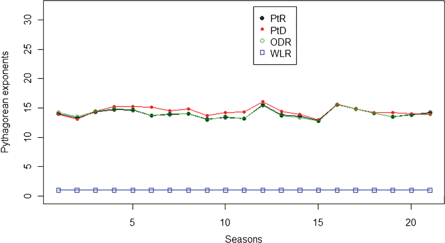
Fig.2
Mean squared error for estimating winning percentage
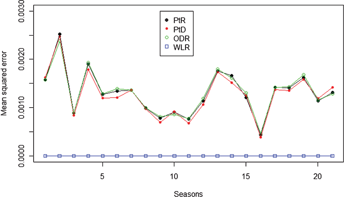
Fig.3
a) Correlation of the strengths with future winning percentage, b) Correlation of log-points ratio with future winning percentage, c) Correlation of log-win-loss ratio with future winning percentage.
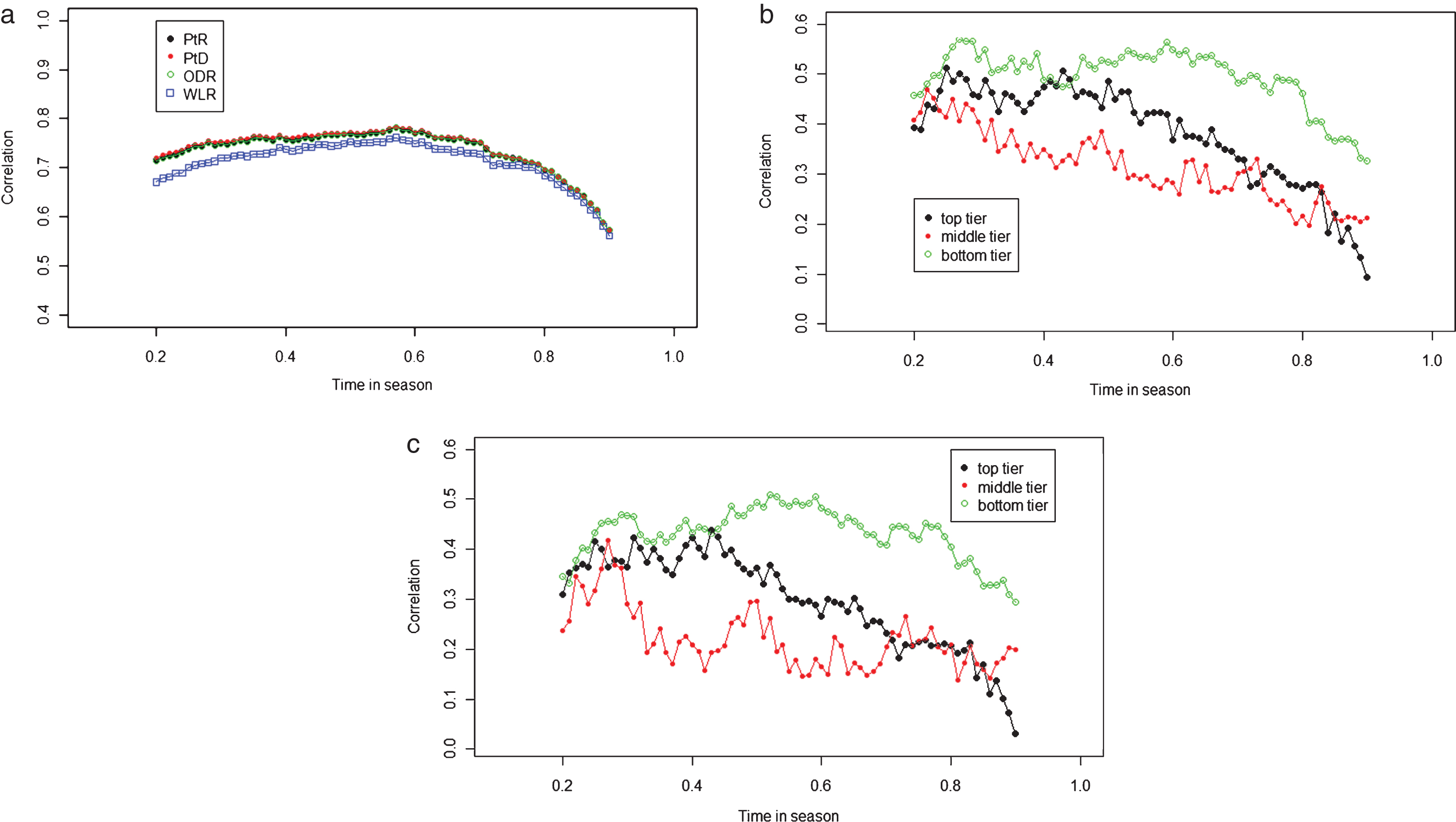
Fig.4
a) Pythagorean exponents for prediction, b) Relative Pythagorean exponents for prediction.
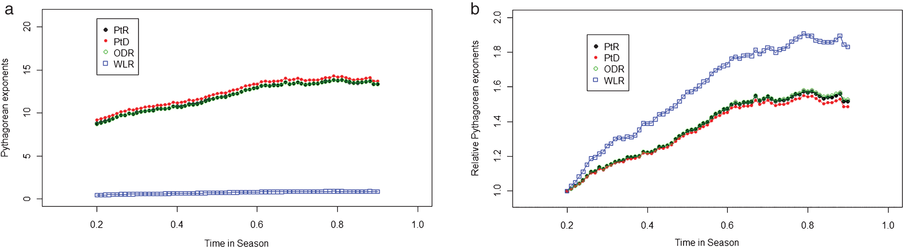
Fig.5
a) Mean squared error of prediction, b) Mean squared error of prediction based on points ratio, c) Mean squared error of prediction based on win-loss ratio.
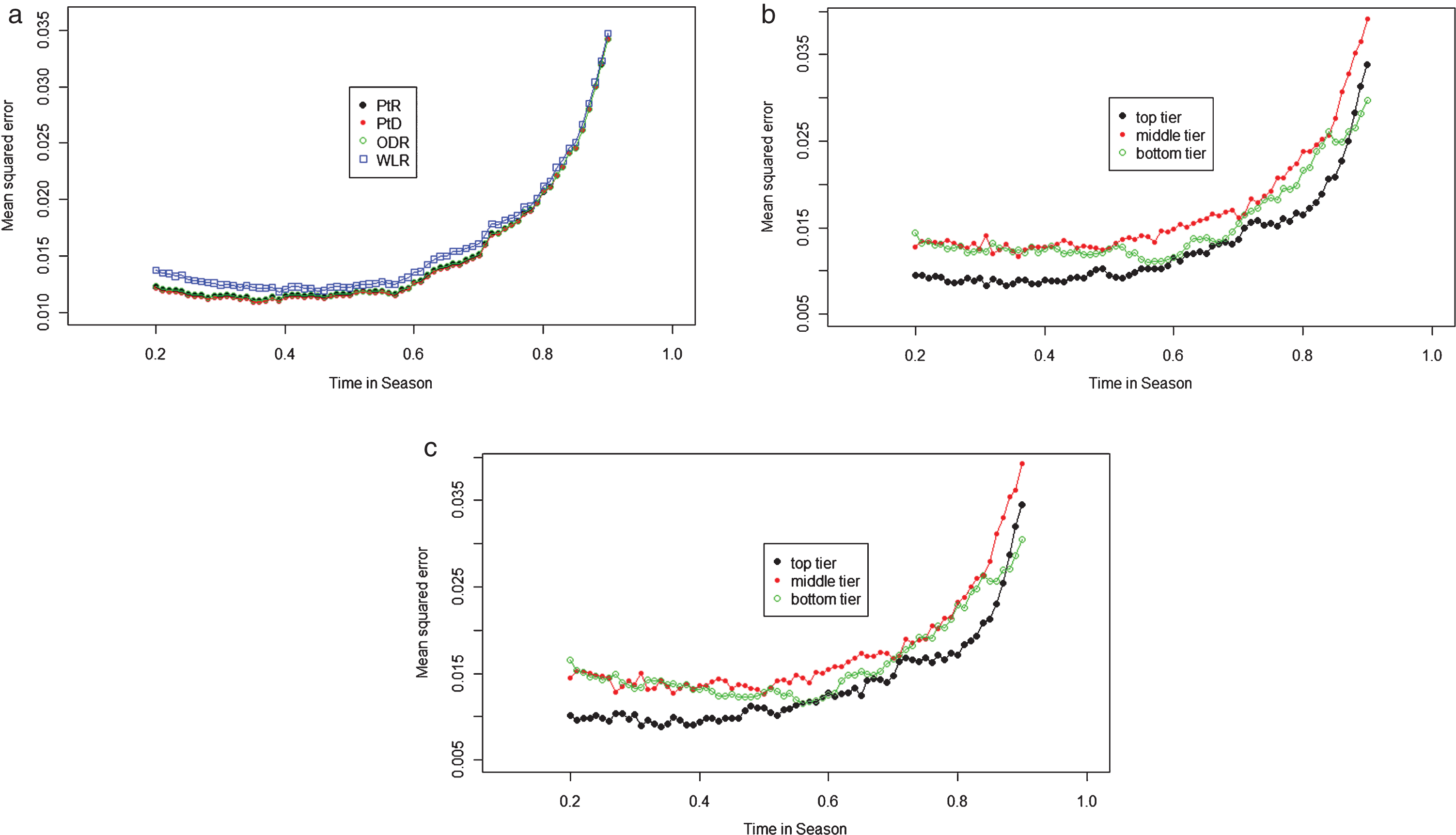
Fig.6
The shrinkage factor of the Pythagorean exponents
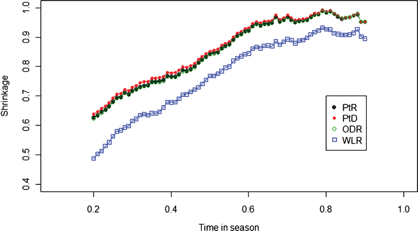
Fig.7
Relative mean squared strengths over times in season.
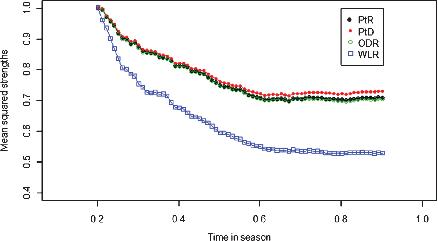
Fig.8
Mean squared logarithm of future win-loss ratio.
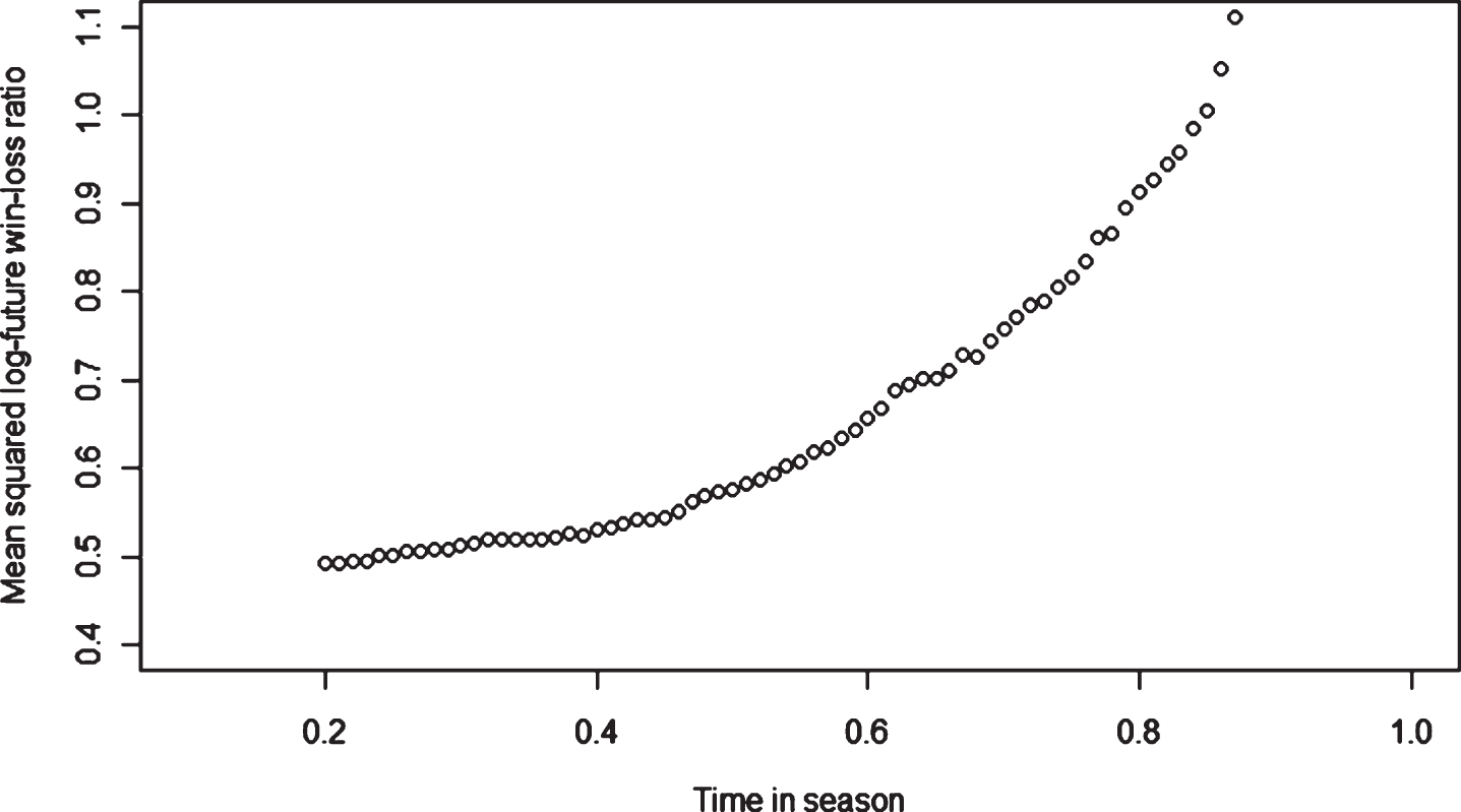
Fig.9
Relative cross product over time in season.
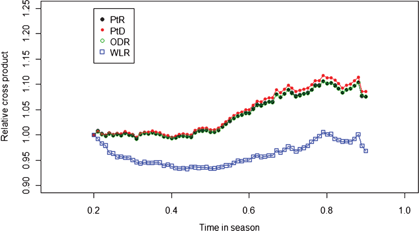
Table 1
Predicted numbers of games won with different Pythagorean exponents and PtR
| Pythagorean exponents | ||||
| PtR | 10 | 12 | 14 | 16 |
| 0 | 41.0 | 41.0 | 41.0 | 41.0 |
| 0.0235 | 45.8 | 46.7 | 47.7 | 48.6 |
| 0.0470 | 50.5 | 52.3 | 54.0 | 55.7 |
| 0.0705 | 54.9 | 57.4 | 59.7 | 61.9 |
| 0.0940 | 59.0 | 61.9 | 64.7 | 67.1 |
Table 2
Summary of the strength measurements with all 21 seasons combined
| PtR | PtD | ODR | WLR (Response) | |
| Mean | 0.000 | 0.000 | –0.000 | –0.006 |
| Standard deviation | 0.047 | 0.046 | 0.047 | 0.687 |
Table 3
Correlation matrix of the strength measurements with all 21seasons combined
| PtR | PtD | ODR | WLR (Response) | |
| PtR | 1.000 | 0.999 | 1.000 | 0.971 |
| PtD | 0.999 | 1.000 | 0.999 | 0.971 |
| ODR | 1.000 | 0.999 | 1.000 | 0.970 |
| WLR (Response) | 0.971 | 0.971 | 0.970 | 1.000 |
| Winning percentage | 0.971 | 0.972 | 0.971 | 0.998 |
Table 4
Pythagorean exponents and least squares fit with all 21 seasons combined
| PtR | PtD | ODR | WLR | |
| Pythagorean | 14.01 | 14.38 | 14.02 | 1 |
| exponents | ||||
| Standard error | 0.140 | 0.142 | 0.141 | 0 |
| 95% confidence | [13.73, | [14.10, | [13.74, | [1,1] |
| interval | 14.28] | 14.66] | 14.30] | |
| R-squared | 0.941 | 0.943 | 0.942 | 1 |
| Mean squared | 0.0013 | 0.0013 | 0.0013 | 0 |
| error |
Table 5
Summary of the season-by-season Pythagorean exponents across 21 seasons
| PtR | PtD | ODR | WLR | |
| Mean | 13.99 | 14.39 | 14.00 | 1 |
| Median | 13.85 | 14.26 | 13.98 | 1 |
| Minimum | 12.86 | 12.97 | 12.77 | 1 |
| Maximum | 15.52 | 16.08 | 15.50 | 1 |
| Standard deviation | 0.718 | 0.774 | 0.740 | 0 |
Table 6
Summary statistics of the Pythagorean exponents over time in a season
| PtR | PtD | ODR | WLR | |
| Mean | 11.96 | 12.40 | 11.95 | 0.772 |
| Median | 12.26 | 12.71 | 12.25 | 0.800 |
| Minimum | 8.780 | 9.203 | 8.750 | 0.488 |
| Maximum | 13.83 | 14.27 | 13.84 | 0.932 |
| Standard deviation | 1.575 | 1.570 | 1.580 | 0.132 |
Table 7
The shrinkage and mean squared errors of prediction for PtR
| Time in season | 0.2 | 0.3 | 0.4 | 0.5 | 0.6 | 0.7 | 0.8 | 0.9 |
| Pythagorean | 8.7804 | 10.049 | 10.733 | 11.804 | 12.926 | 13.559 | 13.763 | 13.319 |
| Standard error | 0.3490 | 0.3608 | 0.3750 | 0.4004 | 0.4398 | 0.4904 | 0.5866 | 0.7854 |
| Shrinkage factor | 0.6267 | 0.7173 | 0.7661 | 0.8426 | 0.9227 | 0.9679 | 0.9824 | 0.9507 |
| Mean squared error | 0.0123 | 0.0114 | 0.0114 | 0.0116 | 0.0127 | 0.0151 | 0.0207 | 0.0341 |
| MSE.14 | 0.0159 | 0.0134 | 0.0127 | 0.0123 | 0.0129 | 0.0152 | 0.0208 | 0.0344 |
| MSE.16.5 | 0.0192 | 0.0161 | 0.0150 | 0.0139 | 0.0141 | 0.0162 | 0.0219 | 0.0359 |
Table 8
The shrinkage and mean squared errors of prediction for WLR
| Time in season | 0.2 | 0.3 | 0.4 | 0.5 | 0.6 | 0.7 | 0.8 | 0.9 |
| Pythagorean | 0.4887 | 0.6163 | 0.6789 | 0.7676 | 0.8444 | 0.8927 | 0.9261 | 0.8945 |
| Standard error | 0.0220 | 0.0242 | 0.0253 | 0.0275 | 0.0308 | 0.0348 | 0.0408 | 0.0545 |
| Shrinkage factor | 0.4887 | 0.6163 | 0.6789 | 0.7676 | 0.8444 | 0.8927 | 0.9261 | 0.8945 |
| Mean squared error | 0.0138 | 0.0125 | 0.0121 | 0.0122 | 0.0136 | 0.0161 | 0.0212 | 0.0347 |
| MSE.1 | 0.0211 | 0.0161 | 0.0144 | 0.0134 | 0.0142 | 0.0165 | 0.0215 | 0.0352 |
Table 9
Pythagorean exponents and prediction for adjusted PtR
| Time in season | 0.2 | 0.3 | 0.4 | 0.5 | 0.6 | 0.7 | 0.8 | 0.9 |
| Pythagorean.25 | 37.935 | 43.552 | 45.829 | 50.262 | 54.842 | 57.866 | 59.014 | 56.289 |
| Pythagorean.50 | 18.864 | 21.226 | 22.346 | 24.451 | 26.657 | 27.913 | 28.322 | 27.251 |
| Pythagorean.75 | 12.038 | 13.681 | 14.530 | 15.947 | 17.432 | 18.268 | 18.537 | 17.903 |
| MSE.25 | 0.0132 | 0.0118 | 0.0116 | 0.0119 | 0.0127 | 0.0150 | 0.0204 | 0.0343 |
| MSE.50 | 0.0119 | 0.0111 | 0.0112 | 0.0115 | 0.0125 | 0.0149 | 0.0205 | 0.0341 |
| MSE.75 | 0.0121 | 0.0113 | 0.0113 | 0.0115 | 0.0126 | 0.0150 | 0.0206 | 0.0341 |
Table 10
Pythagorean exponents and prediction for adjusted WLR
| Time in season | 0.2 | 0.3 | 0.4 | 0.5 | 0.6 | 0.7 | 0.8 | 0.9 |
| Pythagorean.25 | 2.5854 | 3.1158 | 3.3200 | 3.6752 | 4.0137 | 4.2524 | 4.3989 | 4.2082 |
| Pythagorean.50 | 1.2582 | 1.4833 | 1.5913 | 1.7605 | 1.9093 | 2.0096 | 2.0708 | 1.9989 |
| Pythagorean.75 | 0.7614 | 0.9170 | 0.9962 | 1.1100 | 1.2081 | 1.2735 | 1.3147 | 1.2715 |
| MSE.25 | 0.0143 | 0.0126 | 0.0123 | 0.0124 | 0.0134 | 0.0158 | 0.0208 | 0.0346 |
| MSE.50 | 0.0132 | 0.0120 | 0.0118 | 0.0120 | 0.0133 | 0.0158 | 0.0209 | 0.0345 |
| MSE.75 | 0.0134 | 0.0122 | 0.0119 | 0.0121 | 0.0134 | 0.0159 | 0.0211 | 0.0345 |
Table 11
The shrinkage and mean squared errors of prediction for the Bradley-Terry strength
| Time in season | 0.2 | 0.3 | 0.4 | 0.5 | 0.6 | 0.7 | 0.8 | 0.9 |
| Pythagorean | 0.2627 | 0.3718 | 0.6154 | 0.7023 | 0.7788 | 0.8248 | 0.8590 | 0.8225 |
| Standard error | 0.0157 | 0.0196 | 0.0225 | 0.0249 | 0.0279 | 0.0317 | 0.0373 | 0.0500 |
| Shrinkage factor | 0.2875 | 0.4068 | 0.6734 | 0.7685 | 0.8523 | 0.9026 | 0.9400 | 0.9000 |
| Mean squared error | 0.0153 | 0.0137 | 0.0119 | 0.0121 | 0.0133 | 0.0159 | 0.0209 | 0.0346 |
| MSE.0.9 | 0.0229 | 0.0162 | 0.0143 | 0.0132 | 0.0138 | 0.0161 | 0.0210 | 0.0351 |
Table 12
Prediction of game-by-game outcomes
| PtR | PtD | ODR | WLR | BT | |
| Accuracy (h = 0.5) | 0.662 | 0.662 | 0.662 | 0.655 | 0.654 |
| Deviance (h = 0.5) | 1.234 | 1.233 | 1.235 | 1.244 | 1.270 |
| Accuracy (h = 0.6) | 0.682 | 0.683 | 0.661 | 0.683 | 0.680 |
| Deviance (h = 0.6) | 1.184 | 1.183 | 1.224 | 1.185 | 1.216 |

