
Detecting and learning city intersection traffic contexts for autonomous vehicles
Abstract
According to Business Wire, the global market for Autonomous Vehicles estimated at 6.1 thousand Units fpsin the year 2020, is projected to reach a revised size of 110.1 thousand Units by 2026, growing at a CAGR of 60.6% over the analysis period. This strong demand brings more research interests in autonomous vehicle systems. One of the hot topics is autonomous machine vision system and intelligent solutions. Most existing papers on autonomous vehicle machine vision systems apply machine learning models to address automatic object detection and classification issues to support automatic street traffic object detection and classification for vehicles, people/animal, traffic road signs, and signals. However, there is a lack of research results addressing automatic detection and classification of road contexts and transportation intersections under diverse weather conditions. In this work, we present an integrated machine learning model to address the issue and need in street intersection detection and classification based on road contexts and weather conditions. This paper reports our efforts in data collection, processing, and training based on existing data sets (such as BDD100k and COCO), and add a new training data set on street contexts and intersections (13 classes) and weather conditions (6 classes). This paper proposes a 2-stage integrated model to support the detection and classification of different types of traffic contexts and transportation intersection. In the first stage, two deep learning models (Yolo4 and Mask CNN) with transfer learning technique are used to detect the traffic signs, traffic lights, crosswalk and road direction targets on the road in addition to mobile objects (such as people and cars). Later, the generated results from the first stage are used as inputs to a decision tree model to detect and classify the different types of underlying transportation intersections. According to presented experimental results, the proposed 2-stage model receives a high accuracy, so it has strong potential application in computer vision technology of autonomous driving.
1.Introduction
Following the rapid urbanization in modern society, the aspect of transportation has brought public attention. Cars are one of the most important and major transportation tools that largely benefit human lives, providing convenience and efficiency in travel and commuting. However, According to the official record, nearly 40,000 people in the United States died from car accidents in 2017 and around 90% of accidents could be attributed to human error [10]. Some human factors that are commonly regarded as major causes of traffic accidents include memory lapses, the impaired judgment, distraction, delayed or false sensation. While human drivers might be careless, unaware of the coming emergencies, with sufficient training and simulation, an autonomous car learns to identify the potential scenarios and react in real-time. Autonomous cars were firstly introduced in 1939 starting from a fresh electric AV car. The autonomous vehicle is well-known as a self-driving car with full automation to read the signal from the surroundings and operates itself with limited human intervention. However, according to the Society of Automotive Engineers (SAE) international, driving automation can be divided into different levels from 0 to 5. The automation level under 3 is monitored majorly by human drivers; whereas the cars with automation levels above 3 tend to rely more on the automated driving system. Level 5 automation is the so-called “full self-driving” or autonomous vehicle that allows the car to operate appropriately in any condition. While level 3 and 4 automations still require some human input to avoid potential dangers, most of the market players are considering skipping level 3 and jumping to level 5 directly.
After decades of research and exploring the autonomous vehicle, a variety of technologies that assists self-driving were developed and continued to mature the market. According to the global autonomous vehicle market analysis published by Allied Market Research, global autonomous vehicle market analysis will be around 556.67 billion in 2026, giving a CAGR (the compound annual growth rate) of 39.47% from 2019 [21]. To look closely on different levels of automation vehicles, Fig. 1 created by Telecom Italy [33] has illustrated the level of autonomous car sales that have been predicted to have a continually increasing trend. Especially, the L4 and L5 cars are predicted to have skyrocketed sales starting from 2025. Until 2030, L4 and L5 will have estimated over 80 million in unit sales. These statistics show that autonomous cars will have massive market needs and the autonomous driving industry will continue to flourish.
By seeing the huge market potential, budding safe, secure, and highly responsive solutions to support autonomous driving is necessary. It requires a detailed understanding of the driving environment and is the most critical criteria in the initial solution building stage. According to the annual report published by the Federal Highway Administration (FHA), around 40% of all crashes involved intersections in the United States. What’s even worse, a quarter of all traffic deaths and about half of all injuries in the United States occur at intersections [1]. Given such a fact, intersection safety became one priority over road safety. A successful self-driving system should be able to drive in different traffic scenarios without human interruption. These scenarios also include random items near roads or intersections, such as “dumped cardboard boxes” [32]. Among different traffic scenarios, intersections could be the challenging one to learn because of the heavy cars flow and multiple cars could meet or cross on the same path.
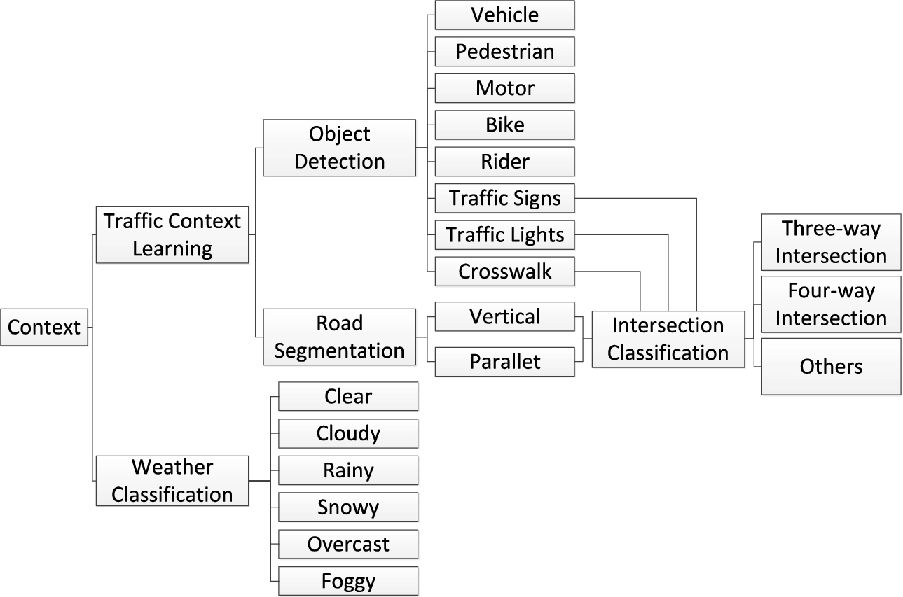
Considering the problems described above, the project aims to provide more understanding in learning the traffic context of road intersections at city streets. The objectives in the project include: (1) Apply deep learning techniques to build models for object detection and recognition in autonomous driving. At this stage toward the goal, we proposed different object detection models in classifying all the on-road objects at the intersection such as multiple types of vehicles, pedestrians, traffic signs and lights, road obstacles and bikes etc. The object detection model will also be extended to recognize different light status and read traffic sign contexts. (2) The next stage is to detect lane direction. This stage classifies the road lanes into two types: parallel and verticals. (3) Performing intersection indicator detection. At this stage, objects need to be detected in more detail. Unlike the regular object detection, all objects which can help with intersection type classification will not only be detected and they will be also detected for their status. For example, traffic lights as one of the most important road intersection indicators will be detected whether there is a front facing or left facing or right facing traffic light. (4) To extend the intersection indicator detection task further, we utilize these indicators to develop an intersection type classification model to assist with driving decisions. (5) Lastly, this research provides weather types by developing a weather type classification model. (6) Based on the results from the previous objectives, all models will be stacked together to provide a summary to define the city traffic context at each road intersection in order to support autonomous driving scenario generation. At the end of the project, we proposed an integrated city traffic context learning solution with condition tables and demo system.
The main contributions of this paper can be summarized as follows. Firstly, a comprehensive system is developed to detect and identify objects and key indicators on the road to assist the traffic situation learning system. The second contribution is that we provide a decision table to support image/video traffic context learning, which can accurately identify multiple types of intersections. The third contribution is to propose an edge computing framework combined with weather scene correction for in-depth learning of Intelligent City assisted driving. The significance of this paper is strong potential of the 2-stage integrated model for application in computer vision technology of autonomous driving and in improving the safety and automation of autonomous driving systems in the future.
The rest of the paper is organized as follows: In Section 2 we introduce the related work of road feature recognition, depth learning and edge calculation. In Section 3 we introduce the acquisition and processing of experimental data. In Section 4 we discuss the traffic objects detection and road segmentation. In Section 5 we discuss the indicator detection and intersection classification. In Section 6 we introduce the performance evaluation of the model. Finally, in Section 7 we make our concluding remarks.
2.Related works
2.1.Machine learning models for autonomous driving
In the field of autonomous driving, deep learning has been utilized and developed in many researches and studies to work on traffic object detection and classification, traffic light and signs recognition and all other related topics. The common deep learning models are usually categorized into one-stage and two-stage detector models. Both these types of models are the most common methods for traffic object detection and recognition.
The model YOLO (you only look once) is the representation of one-stage detector models. The major deficiency of one-stage detectors is that they struggle with small objects within the images, especially for those located at the same grid cell or overlap with other objects. The YOLO pipeline divides the input image into an
All CNN-based models are considered as two-stage detector models. Apart from the traditional CNN model, R-CNN model is a new and fresh approach in dealing with feature extraction in object detection. Compared to the traditional CNN model used in object detection, R-CNN takes advantage of the region proposals and reduces the computational cost. It provides an advanced approach in detecting objects, and it can generate a convolutional feature map. The features are only extracted from the entire image once, and they are sent to the model for classification and localization. This can help with saving a large amount of time for model processing and features storing. Faster-RCNN is another extensive method that replaces the selective search method with a region proposal network (RPN). This novel approach enhances the efficiency of extracting region proposals. Lastly, an extending work to Faster-RCNN that came to our attention is Mask R-CNN. The major contribution of Mask R-CNN is the instance segmentation task. At the second stage, Mask-RCNN adds a third branch in parallel to output the object mask. Instead of using RoIPool from each candidate box to extract features, Mask RCNN applies RoIAlign, which preserves the exact spatial locations of the objects and improves mask accuracy.
To better understand and review different deep learning models, Table 1 summarizes all the models we have mentioned above. Also, it includes different literature reviews for using these models to do specific autonomous driving tasks.
Table 1
Existing deep learning models comparison
| Ref. | DL model | Vehicle detection | Pedestrian detection | Traffic/Sign/Light detection | Traffic sign recognition | Distance estimation | Parameters | Data source |
| [3] | YOLOv4 | Yes | Yes | Yes | No | No | Generic objects | COCO dataset |
| [26] | Mask R-CNN | No | No | Yes | Yes | No | Traffic signs | DFG dataset |
| [14] | Faster-R CNN | Yes | Yes | Yes | Yes | No | A variety of vehicles, person and traffic sign/light | BDD100 K dataset |
| [34] | Canny edge detector | No | No | Yes | Yes | Yes | Not Specified | Not specified |
| [29] | Faster-RCNN inception v2 | No | No | Yes | Yes | No | Traffic signs | GTSRB dataset |
Except for the models mentioned above, there are other many existing deep learning models that have been developed for image classification as well. Especially, starting in 2010, many excellent image classification models have been developed during the ILSVRC challenge competition each year. These models include such as Vgg-16, ResNet etc. All the classification models created during the competition are able to detect 1,000 categories with roughly 1.2 million training images, 50,000 validation images, and 150,000 testing images. Based on these excellent works, the project can utilize them to do a transfer learning for our weather type classification task [25].
2.2.Existing technical solutions
The massive market needs for autonomous cars and continuing growing interests from the public trigger many companies to start to develop and test their own autonomous driving systems. Companies such as Tesla, Waymo, GM cruise have conducted their own AV studies and projects. Among all the automakers, Tesla is the pioneer that stands out from the others because of the ambitious speech given by their CEO, Elon Musk, suggesting that Tesla will become fully autonomous by the end of 2020. Although that didn’t come true, their device named “Autopilot” provides one of the most advanced solutions with great precision. The strong features make Tesla become the big one in the automation industry and people are looking forward to seeing the state-of-the-art solution in the near future [9].
The Table 2 summarizes the state-of-art autonomous driving solutions. It includes five of the top companies who are currently in the top game of AV development and their current levels of automation systems are being tested. Table 2 also describes what features that each AV system supports.
The existing technical solutions lack accurate identification of road intersections in urban traffic environment. Especially in different traffic scenes, heavy vehicles may meet or cross with multiple other vehicles on the same path, which cannot well support the generation of automatic driving scene.
Table 2
Current autonomous driving technologies and solutions
| System name | Data source | Object detection | Traffic sign/Light recognition | Distance estimation | Other features | Testing location/Miles | Level of automation |
| Tesla Autopilo | Camera, ultrasonic | Yes | Yes | Yes | Monocular depth | – Over 2 billion miles | Level 5 |
| NVIDIA DRIVE™ AV Software | Camera, LiDAR, radar | Yes | Yes | Yes | Path detection | – Multiple cities in U.S. | Level 5 |
| Waymo | Camera, LiDAR, radar sensors | Yes | Yes | Yes | Speed detection | – Phoenix, AZ, USA; Santa Clara, CA, USA – Over 32 million kms in real world | Level 4 and 5 |
| GM Cruise | Camera, long-range LiDAR, short-range LiDAR, Articulating radar | Yes | Yes | Yes | Path planning | San Francisco, CA, USA – Over 2 million miles in real world | Level 4 |
| Argo AI | LiDAR, sensor, camera and radar | Yes | City data | City data | City data | – Pittsburgh and Dearborn, MI, USA; Miami, FL, USA; Washington, DC, USA; Austin, TX, USA – Miles not specific | Level 4 |
3.Data engineering
3.1.Data preparation
This project utilizes different datasets in order to provide all the intersection context elements which include various object detection, lane direction detection, and road intersection type and weather type classification. The plan for data collection is mainly divided into two parts. The first part is searching through the existing datasets and the second part is to collect real intersection data on our own. After the data collection, data preprocessing, transformation and preparation will be performed accordingly to both types of raw data. Figure 1 shows the flowchart which summarizes the entire data process of this project.
Fig. 1.
Data process flowchart.
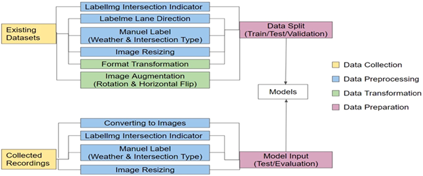
In order to detect objects above the road at the intersection, we have searched online and browsed through different object datasets. We want the existing object datasets to include more traffic related objects. The existing dataset should include images or videos which the bounding boxes labeled surround in each detectable object to show the identity of each object. This allows us to feed the images into different object detection models such as YOLO and RNN based models and train the model to classify the objects at each road intersection. However, there are no existing datasets which have all the objects we want labeled. Therefore, data preprocessing kicks in after we have collected all the existing datasets. Some of the data preprocessing steps we have taken are creating the bounding boxes for objects that we wanted to detect by using Labellmg and Labelme. We also classify the weather type and intersection type images and create the label on our own. Lastly, we made all the images to have consistent size before training them into the models.
Besides utilizing the existing datasets provided by previous researchers, we want to collect our own data in the real traffic environment in order to test our deep learning models. Therefore, we will install one dash camera inside our car at the front windshield to collect our driving recordings within the city of San Jose. After collecting the raw recording, we preprocess the recorded video and transform it into multiple images with the rate of 60 frames per minute.
After defining the data process, we collected a variety of video/image driving datasets for object detection, intersection indicators detection, and weather classification from multiple open sources. Some popular driving data that are commonly used in supporting autonomous driving are Berkeley DeepDrive(BDD100k), KITTI, Cityscapes, ApollowScape, Waymo, ExDARK, MIT traffic and COCO. The data collected by a real driving system is large-scale and contains diverse images/videos captured on the street. The comparison of multiple datasets is shown in Table 3. The ones highlighted are the datasets we chose to use in this research.
Table 3
Comparison between datasets for object detection
| Data | BDD100K | KITTI | Cityscapes | Apollow scape | Waymo | ExDAR | MIT Traffic | COCO |
| # of categories | 10 | 8 | 30 | 25 | 4 | 12 | 12 | 80 |
| Car | Yes | Yes | Yes | Yes | Yes | Yes | Yes | Yes |
| Bus | Yes | No | Yes | Yes | No | Yes | Yes | Yes |
| Truck | Yes | Yes | Yes | Yes | No | No | No | No |
| Van | No | Yes | No | No | No | No | Yes | No |
| Trailer | No | No | Yes | No | No | No | No | No |
| Caravan | No | No | Yes | No | No | No | No | No |
| Motor | Yes | No | Yes | Yes | Yes | Yes | Yes | Yes |
| Bike | Yes | No | Yes | Yes | No | Yes | Yes | Yes |
| Tricycle | No | No | No | Yes | No | No | No | Yes |
| Rider | Yes | Yes | Yes | Yes | Yes | No | Yes | No |
| Pedestrian | Yes | Yes | Yes | Yes | Yes | Yes | Yes | Yes |
| Animal | No | No | No | No | No | No | No | Yes |
| Traffic sign | Yes | No | Yes | Yes | Yes | No | Yes | Yes |
| Traffic light | Yes | No | Yes | Yes | No | No | Yes | Yes |
| # of image | 100,000 | 14,999 | 7,000 | 147,000 | NA | 7,363 | 118,800 | 123,287 |
| Image size | 1280 × 720 | 1382 × 512 | NA | 3384 × 2710 | NA | NA | 4096 × 2160 | NA |
| GPS/IMU | Yes | Yes | Yes | Yes | No | No | No | No |
| Cities/Locations | New York, Berkeley and San Francisco, USA | Karlsruhe, Germany | 50 cities | Mainly in Beijing, China | NA | NA | NA | NA |
| Multiple weathers | Yes | No | No | Yes | Yes | No | Not sure | Not sure |
| Source | 17 | 18 | 19 | 20 | 21 | 22 | 23 | 24 |
From the comparison table, we summarized our findings and have made a decision on choosing the below data:
– BDD100K: It contains large-scale and diverse images with rich annotations in weather conditions, GPS locations, and tags for objects. In addition, the documents and related papers are sufficient so we think it will enhance the understanding of the data and facilitate the project progress. The shortcoming of the data is that it focuses on the traffic objects such as traffic signs, pedestrians, vehicles and riders and doesn’t detect other objects that rarely appear on the road [24].
– COCO: This dataset is widely used in generic object detection and recognition model training. With teons of thousands of images and over 80 object categories covered in the data, the comprehensiveness makes it a great source to detect generic objects such as animals.[15]
– Data we provide: For our collected recordings, we first cut the videos to JPG images with 10 frame per second (fps) with 1028 × 1028 resolutions, then use labelImg to annotate these images for both intersection indicator model and weather and intersection type models. Finally, we resize the images to keep the same resolution and sizes as existing datasets before feeding them to models.
BDD100k consists of images with high resolution (720P), high frame rate (30fps), and GPS/IMP recordings. The annotated videos/images are collected by tens of thousands of drivers supported by Nexar. In total, there are 100K driving videos with 40 seconds per each, covering Multiple US cities including New York, San Francisco, etc. The benchmarks comprised ten tasks including image tagging, road object detection, lane detection, drivable area segmentation, semantic segmentation, instance segmentation, and others, jointly supporting multitask learning in different domains and purposes. Image tagging are image-level annotations on weather conditions, scene types and times of day. To summarize, six weather conditions are annotated for each image. Weather conditions can strongly impact the hue, saturation, and lightness of a picture, hence it plays a great role in object detection. With city scenes under multiple weather conditions trained on the model, we are able to detect the objects no matter how bad the weather is. Figure 2 shows the overview of the dataset that provides examples from BDD 100k. Road object detection allows users to recognize the objects that appear on the road. The object categories cover the different types of vehicles, pedestrians, traffic signs and light. We have shown the object counts by category in Fig. 3 [19].
![An overview of the BDD100K dataset [9].](https://content.iospress.com:443/media/scs/2022/1-3/scs-1-3-scs220010/scs-1-scs220010-g002.jpg)
![Number of instances of each category, which follows a long-tail distribution [24].](https://content.iospress.com:443/media/scs/2022/1-3/scs-1-3-scs220010/scs-1-scs220010-g003.jpg)
COCO, as the term suggested, is a large-scale common objects dataset supporting object detection, segmentation, and captioning tasks. The data has 1.5 million object instances spread over 80 object categories and 91 stuff categories within 164K images. Compared to the other image datasets that specify on detecting on-road objects, COCO leverages the ability in object detection to common animals and other objects that are captured from everyday scenes. Because dogs, cats, birds, horses, and cows appear on the streets really often and may cause road safety issues, the context learning should include the detection of those animals in order to provide more contextual information to identify the traffic scenarios [6].
In the following we used python to illustrate the annotations of COCO 2017, the annotations are stored in a JSON file that could be viewed as a dictionary in python. The file is split to five subsections, info and licenses are the description of the entire dataset, whereas image, annotations, categories provide the information of individual image, the corresponding annotations for the object detected in the image, and a dictionary for mapping the object category with the id.
After detecting the objects, another task that plays an important role in our entire project is the intersection indicators detection. To prepare data for detecting the indicators, we first defined the 13 indicators. The indicators will be helping us to classify the intersection type within the image, consisting of the front crosswalk, right crosswalk, left crosswalk, one way point to front, one way point to left, one way point to right, front traffic sign, right traffic sign, left traffic sign, no right turn, no left turn, no U turn and stop sign. While the data we collected from open source only has annotations for common objects (BDD100K and COCO 2017) and the crosswalks (BDD100K), but is lacking the traffic sign labels. We gathered another batch of images from the Mapillary Traffic Sign dataset.
Table 4
The BDD100K, COCO 2017 and mapillary traffic sign summary
| Data | BDD100K | COCO 2017 | Our labeled dataset |
| # of categories | 10 | 80 | 13 |
| Categories included | – Traffic objects: vehicles, pedestrians, traffic signs/lights, etc. – Lane marking: crosswalk | – Generic objects: vehicles, people, animals, indoor objects, etc. | – Multiple directions of the traffic light, one-way sign, and the crosswalk – No left turn – No right turn – No U turn – Stop sign |
| # of images | 100,000 | 100,000 | 600 |
| Image size | 1280 × 720 | Not specified | 1280 × 720 |
| Resolution | 720 | Not specified | Not specified |
| Image format | JPG | JPG | JPG |
| Annotation format | JSON | JSON | JSON |
| Size (image + annotation) | 6.5 GB + 53 MB | 25.2 GB | 310 MB |
The Mapillary Traffic Sign Dataset is the world’s largest and most diverse publicly available traffic sign dataset and contains lots of great features. The dataset consists of 100,000 images across the world, with over 52,000 images fully annotated by humans and the remaining part annotated partially using advanced computer vision techniques [17]. We summarized the data information in Table 4.
We use labelImg to add annotation for Mapillary traffic sign dataset (MTSD) including image selection approval, traffic sign localization by drawing bounding box, and class label assignment for each box. Before doing so, we could set three conditions for a proper pre-selection of images annotation, which are: (1) pick the traffic sign images for US regions, (2) to cover images of different conditions and qualities, (3) to include as many signs as possible per image [8].
In addition, we split the dataset into three consecutive tasks with the quality assurance process for the purpose of efficiency and quality improvement. The first task is image approval, which selects the images that fit our pre-selection conditions and discards images with low quality. The second task is sign localization, which allows annotators to localize all traffic signs in images and annotate them with a bounding box. By using the Mapillary API, each image is initialized with bounding boxes of traffic signs for speeding up the annotation process. The annotators can manually annotate all missing traffic lights and correct existing bounding boxes to fit the signs tightly. The third task is sign classification, which will use Faster-RCNN to perform this task. Moreover, based on the existing object properties (dummy for false positive and ambiguous for too small, bad quality and heavily occluded), we provide additional attributes, such as occluded (partial occluded), out-of-frame (cut off by image border), included (sign overlap another bigger sign), and exterior (sign that includes other sign) [20].
Then, Mapillary traffic sign dataset (MTSD) will be split into 36,589 training dataset, 5,320 validation dataset, and 10,544 test dataset, respectively, but the images in test dataset will not be annotated for the evaluation purpose [36]. For the COCO dataset, we will not perform any preprocessing steps, because we will use the pre-trained models using COCO. We will use COCO weight as our initial weight for our models. To preprocess all our dataset, the MTSD, the BDD100K dataset, Coco, and our own datasets, we convert all our dataset into JPG format and resize to the same size and resolution [20].
3.2.Data processing
A large-scale dataset consisting of images with a wider collection of various scenarios, improves the generalization and robustness of models, and inhibits over-fitting issues. Aside from self-generating instances from on-board cameras, we want to develop a series of technologies that enhance the existing dataset, for improving the representativeness of distinction tasks.
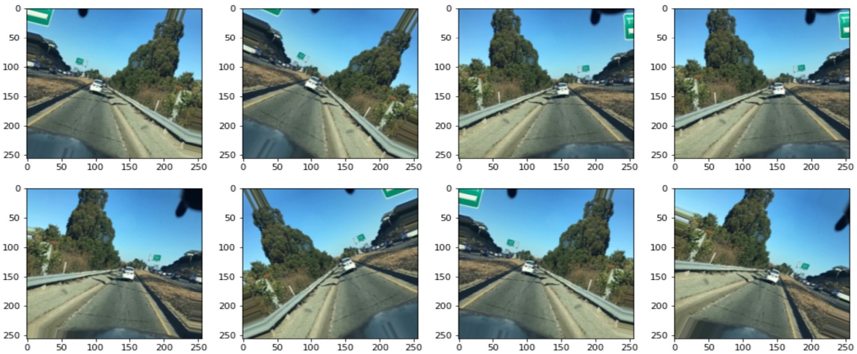
BDD100k consists of images depicting variable classes of weather and time blocks. Weather conditions include six classes: rainy (7125 images), snowy (7888 images), clear (53525 images), overcast (12591 images), partly cloudy (7066 images), foggy (181 images), and undefined. All weather images have been taken among four time blocks: daytime, night, dawn/dusk, undefined. However, the BDD100k dataset do not have very good weather and time blocks. In order to achieve better training performance, images inside the BDD100k will be augmented and used to generate more different weather conditions images. Figure 4 illustrates the tools named ImageDataGenerator, which is a python library we used to apply rotation and flip for our image data. At the beginning, we first normalized images to uniform size, and then utilized ImageDataGenerator to add augmentation effects for increasing weather data variability.
Fig. 4.
Result of data augmentation.
In terms of image annotation, COCO 2017 annotation types for object detection are stored in JSON. In BDD100k, annotations are generated by Scalabel, and follow that Scalabel format, and the 2D bounding box is labeled by box2d. It should be noted that, while the labels in BDD100k are used in JSONs, it is not the same format as COCO. In order to convert annotation format between BDD100k JSON and coco-format, we apply command lines as follow [27]:
– python3 -m bdd100k.label.from_coco -l ${input_file} -o ${out_path}
– python3 -m bdd100k.label.to_coco -m det|box_track -l ${in_path} -o ${out_path}
Fig. 5.
Result of converted COCO.
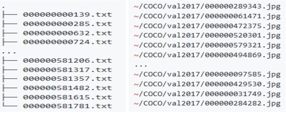
In YOLOv4 Darknet, each image matches one text file, which contains the classes and numeric representations. Before passing our image dataset into YOLO, COCO JSON and BDD100k should be converted into YOLO Darknet TXT format shown in Fig. 5(a). We utilize a Github repo named convert2Yolo, it is created and maintained by Martin and Ben [12]. Convert2Yolo helps convert annotation into Yolo Darkent format [16,18]. It supports four datasets: COCO, VOC, UDACITY Object Detection, and KITTI2D Object Detection. Convert2Yolo requires parameters including name of dataset, image directory path, label directory path, output path, image type, manifest path and darknet *.name file. We apply the command lines to convert coco-format into YOLO Darknet format shown in Fig. 5(b).
$ mkdir ∼/YOLO
python3 test.py –datasets COCO –img_path ∼/COCO/val2017/ –label ∼/COCO/annotations/instances_val2017.json –convert_output_path ∼/YOLO/ –img_type “.jpg” –manifest_path ./ –cls_list_file ∼/COCO/coco.names
The system requires detection and classification models to predict different features. The Table 5 below presents the features and classes of the model to train on the dataset. Object classification has 13 object categories as positive class and object not detected as negative class; Intersection Indicators detection covers over 13 indicators as positive class and object not recognized as negative class.
Table 5
Classes for training/validation set
| Features | # of objects | Positive class | Negative class |
| Object classification | 11 | Car, pedestrian, bus, truck, rider, motorcycle, bicycle, rider, trailer, traffic sign, traffic light | Object not detected |
| COCO object detection | 71 | A diversity of objects | Object not detected |
| Lane segmentation | 2 | Vertical, parallel | Lane not detected |
| Intersection indicators detection | 13 | One way point, left, one way point right, one way point front, left crosswalk, right crosswalk, front crosswalk, front traffic light, right traffic light, left traffic light, no left turn, no U turn, stop sign, no right turn | Object not detected |
| Intersection classification | 3 | 3-way intersection, 4-way intersection, non-intersection | N/A |
| Weather classification | 6 | Clear, partly cloudy, overcast, foggy, rainy, snowy | N/A |
3.3.Data statistics
As we mentioned above, this project uses multiple datasets to perform different tasks. We transform the data first and then split the training, validation and testing datasets to use them to train our models. Datasets such as BDD100k already has the data transformation done, since the dataset already includes different weather conditions and lighting conditions. Therefore, we will not simulate the BDD100K images to include more variations. The Cityscapes dataset was extracted to only include foggy images and it is combined with BDD100k to use for weather type classification. Meanwhile, the BDD100K dataset will be also utilized for object detection and intersection type classification. The Mapillary images are used for annotating different data signs. When using these dataset, we have performed data transformation techniques to increase the variations of the existing images in order to have sufficient training and validation data. Below the Table 6 summarizes the statistics for each dataset:
Table 6
Project used datasets
| Dataset | Features | Original | Transformed | Train | Validation | Test |
| BDD100K | Object detection | 100,000 | 100,000 | 70,000 | 10,000 | 20,000 |
| BDD100K + Mapillary | Intersection classification | 369 | 930 | 525 | 225 | 180 |
| BDD100k + cityscapes | Weather classification | 3,072 | 24,576 | 19,776 | 4,800 | 600 |
| BDD100k + Mapillary | Intersection indicator detection | 600 | 600 | 320 | 100 | 180 |
4.Traffic object detection and road segmentation
We proposed a traffic context learning system diagram in Fig. 6 to provide a clear illustration of the training process. The major task of our solution is learning the traffic context from the street scenes to support scenario generation. There are several components involved: image processing, object detection, road segmentation and intersection classification. In addition to the traffic context learning, we also implemented a weather classification using the Residual Network model to construct potential real-world traffic scenarios.
Fig. 6.
An end-to-end traffic scene context learning system.
Generic object detection aims at locating and classifying objects. In autonomous driving car applications, we include 13 safety-related object classes, 2 classes for lane direction detection, and classes for traffic sign classification. There are two popular methods for generic object detection and classification: one-stage detection models and two-stage detection models. We compared the YOLOv4 and Mask RCNN as below.
YOLOv4, as a one-stage method, is less involved than Faster-RCNN. Two methods both use an anchor box-based architecture. The advantage of YOLOv4 is time efficiency, it is orders of magnitude faster than the Faster-RCNN algorithm. Compared to YOLOv3, rather than using a Feature pyramid network (FPN), YOLOv4 uses CSPDarknet53 as the backbone, which enhances the learning capability of CNN. The spatial pyramid pooling block in YOLOv4 increases the receptive field and capability of separating significant context features [15,24]. Table 7 shows the summarized comparison of models.
Table 7
Comparison of models for object detection/classification
| YOLOv4 | Mask RCNN | |
| Approach | One-stage algorithm | Two-stage algorithm |
| Mechanism | Using a single CNN model to divide an image into regions, and predicting bounding boxes and class probabilities in one evaluation | An extensive work of Faster RCNN focusing on pixel-to-pixel alignment with a novel RoIAlign method |
| Advantages | – Faster than other object detection algorithms – Recognize multiple objects in a single frame – Increase speed and accuracy compare to YOLOv3 – Can be used for real-time task | – Perform instance segmentation: additional branch to output a binary Mask for each RoI – RoIAlign leads to large improvements by experiments – Decouple mask and class prediction to prevent competition among classes – Mask RCNN is faster to implement and train – Can be used for real-time task |
| Disadvantages | – Struggle with small objects – Has minimum size requirement | – Ignore the difference between spatial information between receptive fields of different sizes – The network does not consider the relationship between the pixels at the object edge so those pixels are misclassified |
Mask-RCNN is state-of-the-art in terms of object detection. Similar to Fast-RCNN, Mask-RCNN adopted the identical region proposal network. While, instead of using RolPool, it utilizes ROIAlign to locate the relevant areas of the feature map. It extends the Fast-RCNN architecture with a parallel bounding box recognition branch, and instance segmentations will be generated through another branch at the pixel level. Mask-RCNN model supports both object detection and object segmentation [35].
In autonomous driving application scenarios, there are two main challenges of pedestrian detection. One is accurate object detection of a small object [22]. According to Zhong-Qiu et al., when the Region-of-Interesting pooling layer (Faster-RCNN) is smaller than the export layer, collapsed pooling bins cause “plain” feature extraction [37]. Another challenge is illegible negative instances confused with the background. To tackle these issues, Liliang et al. suggested using high resolution of feature maps and improving Faster-RCNN by adopting RPN followed by boosted forests on shared.
Our solution aims to feed multiple datasets centering on different objects. At the first stage, the Mask RCNN model was implemented for detecting the 13 classes in the BDD100K dataset, which includes vehicle, pedestrians, rider, motor, bike, and so on (The details of the dataset could be found in Section 3). At the second stage, the traffic signs and traffic lights toward different directions, and the crosswalk in the front and on the two sides would be detected using the YOLOv4. While traffic signs and traffic lights are comparatively smaller objects. We adopted several tuning methods to increase the network solution and set up different sets of layers and a number of strides to enhance the detection accuracy.
To start learning the traffic context at road intersections under different scenarios, object detection and road segmentation are implemented. The associated deep learning models being used are described below.
Object detection and Road segmentation (Mask RCNN). As mentioned earlier in literature surveys and existing technologies, RCNN is one of the major applications of CNN to object detection. Mask RCNN is extensive work to the Faster RCNN and is conceptually simple. Similar to Faster RCNN, Mask RCNN adopts the same two-stage procedure. The first stage involved an identical region proposal network which was introduced in Faster RCNN to propose candidate bounding boxes. In the second stage, Mask-RCNN adds a third branch in parallel to output the object mask. Instead of using RoIPool from each candidate box to extract features, Mask RCNN applies RoIAlign, which preserves the exact spatial locations of the objects and improves mask accuracy [11].
At the beginning of the training, the multi-task loss defined in Mask RCNN was
The original paper presented relatively good instance segmentation results by experiments. To achieve that, extracting the spatial structure of masks by pixel-to-pixel correspondence provided by convolution was adopted to encode an input object’s spatial layout. While the pixel-to-pixel behavior requires the RoI features, for those small feature maps to be well aligned to preserve the explicit per-pixel correspondence, the following new improvement RoIAlign layer was developed [30].
About RoI Pooling vs RoI Align. While RoIpool worked very well for Faster RCNN in object detection problems, the slight misalignment between the RoI and the extracted features may have a large negative effect when it comes to pixel-level segmentation. To address this, the RoIAlign layer properly aligns the extracted features with the input by applying Bilinear interpolation to compute the exact values of the input features at four regularly sampled locations in each RoI bin, then aggregated the result using max pooling or average pooling. Figure 7 compares the output feature map from RoIPool and RoIAlign [30].
Fig. 7.
(a) Left: imposing RoIpooling on the feature map and dividing into 2 × 2 grids. Right: output after MaxPooling. (b) Left: applying RoIAlign with the same RoI. Middle: output after bilinear interpolated. Right: output after MaxPooling [30].
![(a) Left: imposing RoIpooling on the feature map and dividing into 2 × 2 grids. Right: output after MaxPooling. (b) Left: applying RoIAlign with the same RoI. Middle: output after bilinear interpolated. Right: output after MaxPooling [30].](https://content.iospress.com:443/media/scs/2022/1-3/scs-1-3-scs220010/scs-1-scs220010-g007.jpg)
The model we proposed in this project was developed in the original paper. The mask RCNN was instantiated with multiple architectures including ResNet and ResNeXt networks of depth 50 and 101 layers. Another effective backbone was FPN, which uses a top-down architecture with lateral connections to build an in-network feature pyramid from a single-scale input. The ResNet-FPN backbone inherits the advantages of both networks and shows greater performance in both accuracy and inference speed [11].
In this research, we started training the model with the pre-trained COCO model. We performed transfer learning with our custom datasets including the BDD100K object detection and road segmentation data.
In the Mask-RCNN model for object detection, the sizes of all the images were 256 × 256, and a total of 10,000 image data. The data were split into 70% for training, 20% for validating, and 10% for testing. For training the BDD100K dataset and Mapillary, we train the model in two stages. We froze backbone layers and randomly initialized layers for 5 epochs with a 0.0001 learning rate that model can cope with 15 output classes (Background, 13 object classes, and 2 lane direction classes of BDD100k). Then fine-tuned the model with all layers for 16 epochs with a 0.0002 learning rate. The batch size was 100, the image per GPU was 1, and it took approximately 2 hours per epoch with Resnet50 as the backbone. After training, we created an inference model and used the recording video we collected in San Jose District 9 to evaluate the model performance.
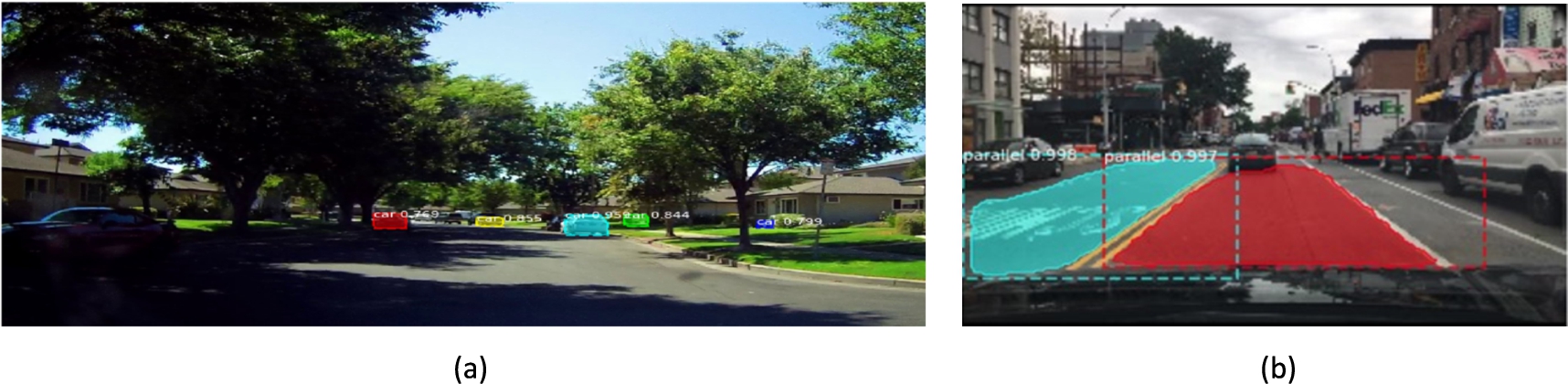
In Fig. 8(a) we present a result example image of a self-generated validation dataset. As we can see the model detected cars parked on both sides of the road, the model has a false prediction box where it wrongly predicts a car instead of a yard chair but also some cars far away that are not detected. We will improve our model by increasing image resolution. After obtaining the optimal hyper parameters, the model will be trained and compared with more layers net (ResNet-101) for optimal performance.
Fig. 8.
(a) Visualization result of Mask RCNN model on a self-generated validation dataset. (b) Lane detection results.
Same as object detection, we use Mask RCNN for lane detection and COCO pre-trained weight as initial weight. For the lane detection, we have the following attributes:
– Lane directions – vertical and parallel
– Vertices – list of x1, y1, x2, y2 points
After relabeling the lane annotation for bdd100, most lanes could be detected, especially the images in an images with clear lane signs, no shades or abstracts shown in Fig. 8(b)
To evaluate the model of our research project, we come with different metrics to make adjustments on each part of model performance. Below are the five basic metrics that we used to evaluate the object detection and also the traffic light and sign detection models. Table 8 shows the summarized comparison of object detection evaluation metrics.
Precision divides the true positives out of all positive prediction results and it evaluates the object detection accuracy and indicates the percentage of correct ones. Recall divides the true positives out of the actual positives and it evaluates how good we can find all the correct objects.
Table 8
Object detection evaluation metrics
| Metrics | Formula | Reference |
| Precision and recall | [31] | |
| TP = True positives, FP = False positives, FN = False negatives | ||
| Intersection over union (IOU) | [13] | |
| Area of intercept = Ground Truth ∩ Prediction | ||
| Area of overlap = Truth ∪ Prediction | ||
| Average precision (AP) | [28] | |
| where | ||
| Mean average precision (mAP) | [28] | |
| Where | ||
| Variations among mAP | Same as above mAP | [28] |
| Frames per second (FPS) | FPS = inference time for all image | [5] |
IoU measures how much that the pre-labeled bounding boxes (ground truth) in the dataset overlap with the prediction bounding box. In general, IoU uses 0.5 as the default threshold. If IoU ≧ 0.5, then the prediction is deemed TP, otherwise, the prediction is FP. AP is range between o and 1 which is the area under the precision-recall curve it evaluates the detection model accuracy. mAP is simply the average of AP and it is also popular to be used to evaluate the object detection model accuracy. The default threshold for mAP IoU is 0.5 which means the model will use 0.5 as the threshold to remove invalide bounding boxes. However, this might not always be the case. mAP small: when 0.25 is the threshold and it should be used when the model detects smaller objects in the dataset. mAP large: when 0.75 is the threshold and it should be used when the model detects larger objects in the dataset. FPS evaluates how fast our model can produce optimal results once the data has been input to the model. IoU is the element to calculate the precision and recall. Once the precision and recall have been calculated for each predicted object category, the precision-recall curve will also be plotted in order to further obtain the AP for each object class. The average will be taken for all the APs among all classes which is known as the mAP. For the traffic light and sign objects, mAP small will be used to set the IOU threshold to be 0.25 since both traffic light and sign are considered small objects. Additionally, FPS will be used to measure the speed of our model to evaluate how fast the model can bring the results to us. Therefore, mAP and FPS are the main matrices that will be used for comparing Regional Convolutional Neural Network (Mask-RCNN) and Faster-RCNN models for object detection and recognition.
As the last objective stated, learning intersection context is also important for the project. Through the object detection and recognition stage, we can learn all the traffic contexts including what types of objects exist in the current intersection and what traffic situation involves regarding signage and traffic light However, knowing what type of road intersection such as a 3-way or 4-way intersection is also important and requires it to be evaluated. In general, we can use the number of corrected intersections being classified divided by the total number of intersections to get the classification accuracy for the intersection.
![Confusion matrix for intersection type evaluation [2].](https://content.iospress.com:443/media/scs/2022/1-3/scs-1-3-scs220010/scs-1-scs220010-g009.jpg)
To look more in detail, a confusion matrix will be created to compare the difference between the predicted intersections with the ground truth for each type of intersection. Figure 9 above illustrates an example of the confusion matrix which will be created for this project to evaluate the intersection type to support context learning.
For Mask-RCNN, we adopt the ResNet101 backbone on MS COCO dataset as our baseline. Against this baseline, we train and test our Mask-RCNN with BDD100K dataset. 256 × 256 input for head layer training with 0.001 learning rate with 10 epochs to increase the computation speed, and tuning the whole model with 1024 × 1024 resolution input to achieve lower loss, and with 0.0001 to make the model converge faster.
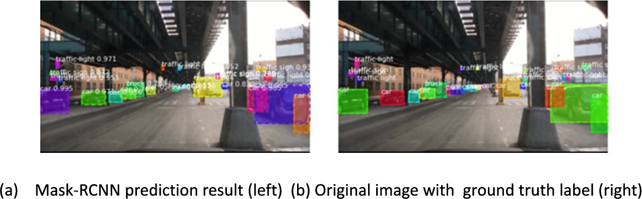
We present an example image of the BDD100K dataset with the predicted bounding boxes in Fig. 10(a), and the actual image in Fig. 10(b). The model provides high confidence and good match for some classes like car, while it can still be improved for small traffic sign recognition, and classes with small training samples like train, motorcycle, and bus.
Fig. 10.
Visualized result of images of BDD100K’s test set.
We evaluate our result by research community-standard performance indicators such as F1-score, mAP which have been mentioned earlier. Table 9 shows the evaluation metrics comparison. The formula below shows the relationship among indicators and computation steps.
Table 9
Evaluation metrics comparison
| Model | mAP | F1-Score |
| Mask R-CNN Baseline | 0.282 | 0.240 |
| Modified Mask R-CNN | 0.565 | 0.479 |
Fig. 11.
Confusion matrix from Mask R-CNN with ResNet101 on BDD100k validation set.
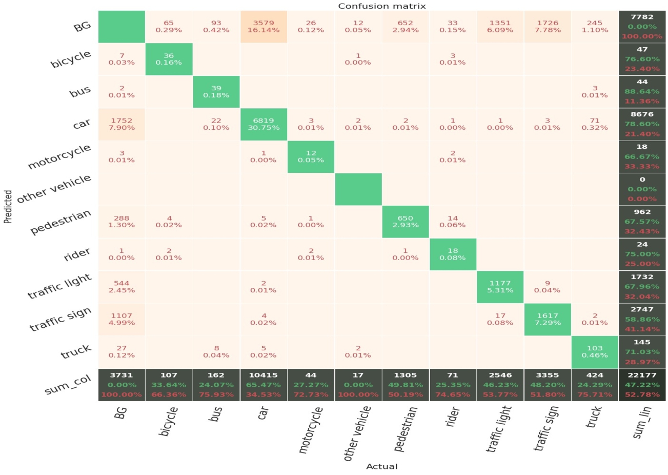
Figure 11 shows the Mask-RCNN model’s confusion matrix based on 0.5 IoU threshold. We evaluate the model with 1000 images from the BDD100K validation set. The y coordinate represents the prediction for each class, and the x-axis represents the true label class. The last column includes the total amount of predicted class and its precision, and the last row indicates the total amount of ground truth, each cell contains count number and recall for the corresponding true class. From the evaluation above, one of the insights we got from the training process is that, imbalance between object training data and data with non-ideal visual conditions would lower the model performance. Therefore, to tackle these issues, we will next enrich and further customize the datasets.
In Mask-RCNN, we used Resnet101 backbones as baseline for lane detection with 0.01 learning rate and 256 × 256 input for 10 head layer training and 500 epochs. Figure 12 represents the detection result. It accurately detects the parallel lanes.
Fig. 12.
Lane detection result.
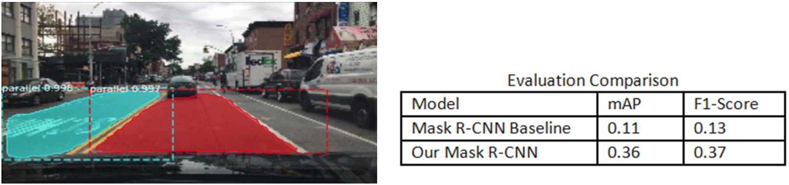
The data to the right in Fig. 12 shows the evaluation metrics comparison for Mask R-CNN baseline and our tuned model. BDD100k has their lane annotations, however, we recognize several issues in their ground truth annotations resulting in low accuracy, due to the small and crowded lanes. Then we decide to draw our annotation using labelme, where the parallel lanes represent the lanes along our driving way, and otherwise we mark the vertical lanes. Although our model mAP and F1-Score have increased slightly from 0.11 to 0.36 and 0.13 to 0.37 respectively, we could improve the model accuracy easily by adding more qualified images and annotations. In selecting the qualified images, we summarize the following suggestions:
– Pick images with clear (dash or solid) road lanes in the image
– Collect more intersection datasets with clear and more vertical lanes.
– Instead of drawing lines for lane, we could draw polygon for bounding box
5.Indicator detection and intersection classification
Referenced to the previous model surveys, a model detector can be categorized into two types. YOLO is one of the most representative models for one-stage object detectors. YOLOv4 consists of a CSPDarknet53 as backbone, a SPP-PAN as neck and a YOLOv3 as head and was tested on ImageNet, MS COCO datasets with different training improvement techniques for data augmentation, regularizations and class label smoothing. The model tested the influence of different training improvement techniques on ImageNet and COCO 2017 datasets. At the beginning stage, two convolutional neural networks CSPResNext50 and CSPDarknet53 are evaluated on the ImageNet and COCO datasets. the requirements of the detector are listed bellows:
– Higher input network size (resolution) – for detecting multiple small-sized objects
– More layers – for a higher receptive field to cover the increased size of input network
– More parameters – for greater capacity of a model to detect multiple objects of different sizes in a single image
While CSPResNext53 only contains 16 3 × 3 convolutional layers, a 425 × 425 receptive field and 20.6 M parameters, CSPDarknet53 has 29 convolutional layers, a 725 × 725 receptive field and 27.6 M parameters. With the experimental result shown after the test, CSPDarknet53 is the optimal model as the backbone for the detector [3]. Aside from the backbone, SPP block was added over the CSPDarknet53 to increase the receptive field and extract the most significant contextual features without any reduction of the operation speed. PANet was used for parameter aggregation from different backbone levels for different detector levels [3]. The architecture of YOLOv4 is illustrated in Fig. 13.
Fig. 13.
Improved model architecture based on YOLO v4.
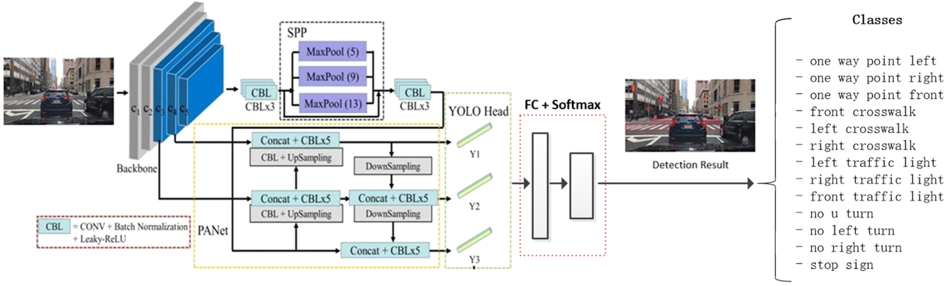
The model was proposed to detect indicator objects including traffic signs, traffic lights in the front, traffic lights on two sides, and crosswalks in different directions. The traffic signs include stop signs, one way, right turn, left turn, no left turn, no right turn. The training data was collected from BDD100K and Mapillary dataset. The intersection images are selected manually and the YOLOv4 labels for each image are generated using LabelImg. The documentation of Darknet suggested we start training on our custom datasets with batch = 64, subdivisions = 16 and set the network size at 416 × 416 at the beginning to speed up the training. In addition, to increase the ability and precision in detecting small objects, we increased the network resolution from 416 to 608 and 832 after thousands of epochs during the detection phase. While the custom objects comprise directional road signs, we disable the flip data augmentation by adding flip = 0 in the configuration.
The proposed models above helped us to detect the objects, traffic signs, and traffic lights on the road, recognize the road types in the street scenes and classify the street scene images by the weather conditions. The next task was to classify what type of intersection within the image, such as a four-way intersection or three-way intersection. This task is critical for learning the traffic context because different intersection types can lead to different driving decisions. For example, a three-way intersection may only allow a driver to make a left turn and no right turn can be made. Therefore, different machine learning algorithms have been implemented to make intersection type classification.
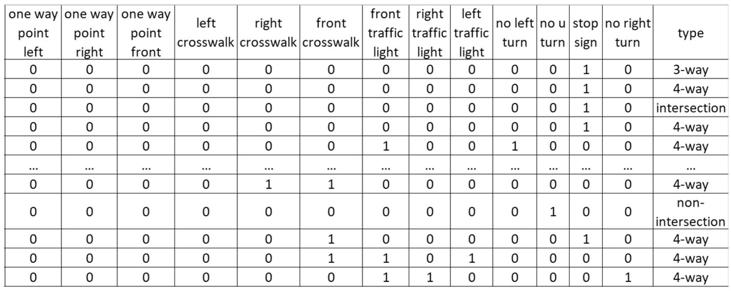
We leveraged the results derived from the indicator detection and road segmentation to determine the intersection scenarios. This solution could be divided into two stages. The first stage was to decide whether the image has an intersection. In an input image, if we detected a vertical road along with a parallel road, we considered the image as an intersection scene and proceeded with the indicator detection. Figure 14 illustrates the process of classifying the intersection. After detecting the indicator objects, each image had its corresponding decision table which indicated whether there’s a traffic light, in which direction there was a traffic light, what crosswalks can be found, and whether there are any special traffic signs indicated there. While the data we collected and labeled manually is imbalanced, we applied the up sampling method to increase the number of minority classes. Figure 15 shows the elements we have included in our decision table. By having all the key information as the classification indicators, we implemented multiple ML models to classify the types of intersections within the images.
Fig. 14.
Two-stage intersection classification.
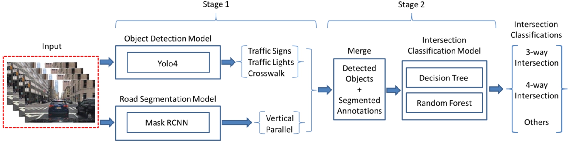
Fig. 15.
Intersection classification input table.
YOLOv4 model was implemented in our integrated system in parallel with the mask RCNN models. While the mask RCNN model is only responsible for comparatively larger and generic objects appearing in the street scene, YOLOv4 trained on the custom dataset covers 13 critical intersection indicator objects. The IoU and mAP (50) score for each class under different network resolution are shown in Table 10. As we gradually increased the network resolution from 416 to 832, the mean average precision improved.
Table 10
Evaluation result of the YOLOv4
| Network resolution | Precision | Recall | F1-Score | IoU | [email protected] |
| 416 × 416 | 0.61 | 0.45 | 0.52 | 45.14 | 45.14 |
| 608 × 608 | 0.66 | 0.6 | 0.63 | 49.89 | 53.35 |
| 832 × 832 | 0.66 | 0.6 | 0.63 | 49.89 | 55.22 |
| 1024 × 1024 | 0.6 | 0.63 | 0.61 | 44.67 | 53.70 |
Table 11
The classification report of decision tree and random forest
| Model | Precision | Recall | F1-score | Accuracy |
| Decision tree | 0.81 | 0.77 | 0.77 | 0.77 |
| Random forest | 0.80 | 0.77 | 0.78 | 0.77 |
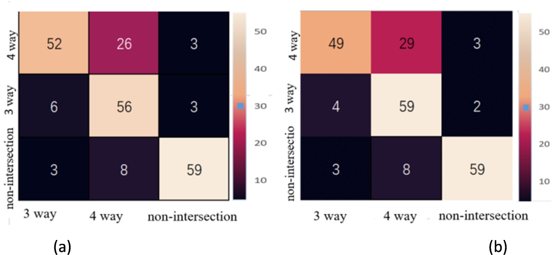
After detecting the intersection indicators on the road, the intersection classification using decision tree and random forest were deployed at the final stage. Table 11 shows the classification results with different metrics. There’s not much difference between the decision tree and the random forest. From the report, the precision of classifying the 3-way intersection scene is comparatively low. Given all images classified as a 3-way intersection, only 60% and 57% of them are correctly classified. Whereas the precision of 4-way intersection has very high accuracy at 92% and 97%. Figure 16 shows the confusion matrix of decision tree and random forest.
Fig. 16.
The confusion matrix of (a) decision tree (b) random forest.
The previous training and evaluation split the 600 images and the indicators into the training set and testing set at ratio 7:3, we also evaluated the model using ten-fold cross-validation. The evaluation result presented in Table 12 shows the fit time, test time, test score. Overall, the decision tree took much less time in training and testing. While the random forest performed a little bit better than the decision tree, it took more than 100 times the decision tree in the training process. To obtain the best performance in both classification accuracy and the run time, grid search was used to determine the parameter combination which best fits our model.
Table 12
Evaluation result on ten-fold cross-validation
| Model | Fit time | Test time | Test accuracy | Test f1-score |
| Decision tree | 0.0042 | 0.0036 | 0.76 | 0.74 |
| Random forest | 0.2188 | 0.0201 | 0.75 | 0.73 |
6.Traffic weather classification
Weather classification is another element that supports the situational analysis of autonomous driving intersections in this study. There are six weather categories in this project which we aim to be able to detect: ‘clear’, ‘overcast’, ‘partly cloudy’, ‘rainy’, and ‘snowy’. Knowing the type of weather will enhance our computer vision system’s ability to recognize road conditions and help the system make driving decisions. This task requires a sophisticated deep learning model which can allow us to use any on-road captured image as the model input and identify the weather classification category as the model output. Many deep learning models have been developed and utilized for image classification. The most common one and also known as the most typical image classification model is the Convolutional Neural Networks (CNN). However, CNN has an issue when adding too many layers of networks. The performance will degrade instead of showing an improvement. However, the Residual Network was introduced after CNN and it is a DNN based neural network with additional layers added. It is not limited by this maximum threshold for depth issue and it can provide better image classification performance.
Therefore, this research proposed to use the residual network models to classify the weather type of the on-road images. We believe by adding more layers, the accuracy of the residual network models should be increased.
The Residual Network model allows for shortcut connect. The input X can be shortcutted to skip those weight layers in the middle and perform identity mapping. As a result, by adding more layers, the accuracy of the residual network models should be increased, not degraded [4]. Therefore, this research proposed to use the enhanced residual network models to classify the weather type of the on-road images.
Fig. 17.
Enhanced ResNet model for image weather classification.
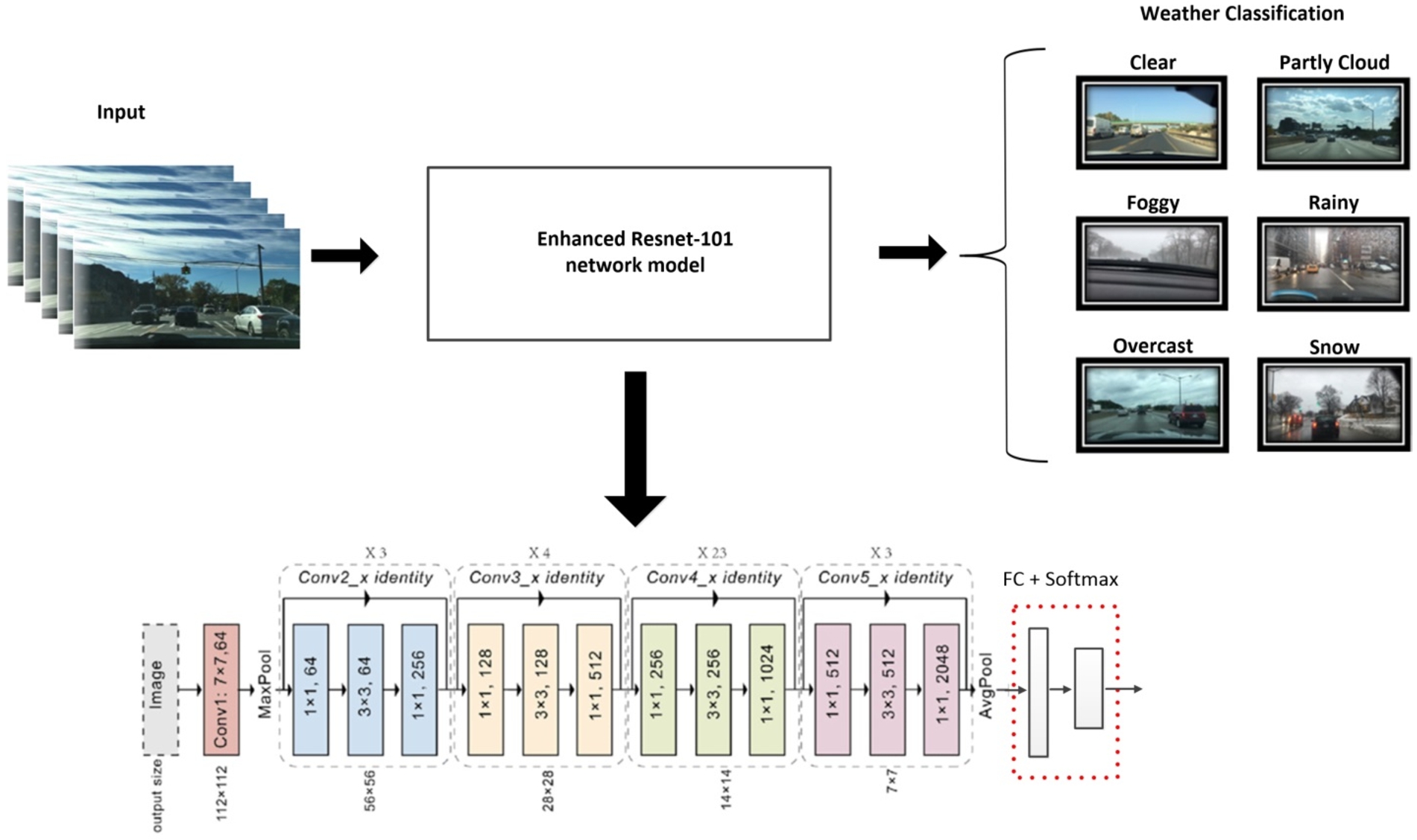
The workflow of using the Residual Network models to train on our BDD100K image is illustrated in Fig. 17. The input image will be imputed into the pre-trained ResNet model. To get accurate classification results, we modified the last few layers of the pre-trained ResNet model. These layers are listed as the following:
– Flatten layer: this layer flattens the output from the previous layer of the neural network and prepares it to fit into the next dense layer.
– Dense layer: the dense layer prepares the model to classify the image into the correct weather category. There are 6 weather categories we would like to identify, so the last dense layer contains 6 columns.
– Batch normalization: this process allows the model to be more robust. It will let those outlier image inputs have less impact on the training process.
– Dropout: This dropout is set to prevent the network from learning from repeatable information by setting the probability to activate a neuron otherwise the neuron will be zero.
As we described above, we used the pre-trained ResNet model to train on our images so that it can classify six weather types. The model implementation and the training process are all coded in Python by utilizing the Keras package. The Keras is a very popular and commonly used neuron network public library that stores many pre-trained ResNet models. The ResNet modes have two versions. Version 2 is enhanced from version 1 by adding batch normalization after each dense layer. In this project, we used version 2 of the ResNet model.
![Architecture of different ResNet models [23].](https://content.iospress.com:443/media/scs/2022/1-3/scs-1-3-scs220010/scs-1-scs220010-g018.jpg)
Additionally, the ResNet model has different types which include different layers. As shown in Fig. 18, the ResNet model has 18-layer, 34-layer, 50-layer, 101-layer and 152-layer. The output size for all ResNet models is the same, but the convolutions layers are added more and more to create deeper depth neuron networks. Ideally, as the network gets more and more layers, the accuracy and model performance should be improved instead of degraded due to the shortcut connection feature that the ResNet model has. Additionally, all the ResNet models have the same process inputs and the images are needed to preprocess before fitting them. After modifying the pre-trained ResNet model and our images get trained and validated, the model output classifies all the images into six categories.
As previously mentioned, in this project we proposed to use both ResNet and VGG pre-trained model as the base model by adding some flatten layers, dense layers, batch normalization, and dropouts to enable the image classification to six weather categories. Additionally, we chose to use ResNet101 and VGG-19. Based on the related research we have mentioned previously, ResNet101 has much better performance than ResNet50 and other types of ResNet models and also VGG-19 seems to have better performance than VGG-16 and the rest of the VGG models. The datasets we used for the weather classification models come from BDD100K and Cityscape foggy datasets. The BDD100K has the weather type labeled images, but the majority of them are not correctly labeled. Therefore, we had to manually re-label each image to the correct weather type. Also, before inputting images into our models, we have pre-processed the images based on the ResNet and VGG model requirement. The VGG and ResNet’s model input have the same format in which the input images need to be seen in the order of height, weight, and number of channels. Additionally, we also tried to do some data augmentation such as rotation and horizontal flips. Table 13 shows the accuracy results from the ResNet101 model compared with the VGG-19 model. The data augmentation has been all included prior to training all the models.
Table 13
Model testing results
| Accuracy | ResNet 101 | VGG-19 |
| Original BDD100k + Cityscape | 68.3% | 68.1% |
| Self-labeled BDD100k + Cityscape | 81.3% | 82.7% |
Table 13 shows the model results for the weather classification. After self-labeling the BDD100K images, the accuracy has been hugely improved. The result shows that ResNet 101 can have a 81.33% of classification accuracy while the VGG-19 model has 82.67%. The VGG-19 model has a slightly higher accuracy than the ResNet 101 model.
Fig. 19.
Confusion matrix from ResNet101 and VGG-19 models.
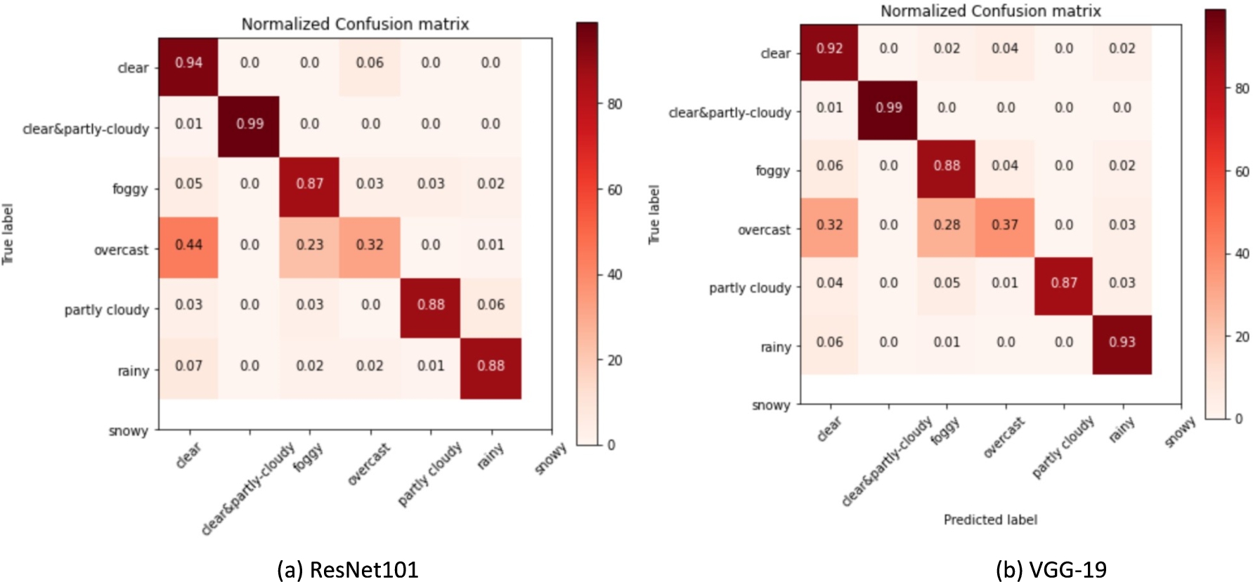
To further evaluate the model classification results, we have also checked the confusion matrix which shows how each weather type has been classified accurately. The confusion matrix for both VGG-19 and ResNet101 are very similar. However, the ResNet101 model is a little bit better on classifying clear and partly cloudy weather type and VGG-19 model seems to have higher classification accuracy on rainy and foggy weather type.
Overall, both models perform pretty well in that each weather type gets to be classified accurately at least 87% of the time except for the overcast weather type. However, based on the model accuracy, we have selected the VGG-19 model to be the best to do our weather type classification.
7.Performance evaluation
We validated the object detection model on 13 common traffic objects. The mAP of the model on the validation set of BDD100K was 57% and the detection outputs with labels deployed on OpenCV showed moderate precision in detecting cars, pedestrians and traffic signs. The weather classification model has a 82.7% accuracy rate on distinguishing the weather shown in the images, the confusion matrix showed that only pictures that were taken under clear weather were correctly classified, whereas the rest of the pictures were mixed up together. To fine-tune the model, we considered reducing the weather classes by combining the cloudy pictures and the clear pictures. The model has improved its accuracy from 68.1% to 82.7%.
To help detect intersections, we detect vertical and parallel road lanes. The current lane detection model has low mAP, and we may need to increase the number of epochs trained from 5 to 30 before training the model, and work on the configuration to improve the model performance. The intersection classifiers relied on the detection results of the YOLOv4 model. The table below shows that the traffic sign, traffic light and crosswalk are great indicators and if the road segmentation and indicator detection model can be successfully implemented, the intersection types can be accurately detected. Figure 19 shows the confusion matrix from ResNet101 and VGG-19 models.
We planned to evaluate the models in two ways. The first one is to validate the results by comparing the prediction and the ground truth of the validation set. The second one is to use OpenCV to create a demo of our recordings in San Jose Downtown. The evaluation result comparison is shown in Table 14.
Table 14
Model improvement comparison
| Features | Model | Validation accuracy | Test accuracy | |
| Traffic | Common objects | Mask RCNN | 0.69 mAP (@IoU=0.5) | 0.71 mAP (@IoU=0.5) |
| Road types | Mask RCNN | 0.7 mAP (@IoU=0.5) | 0.36 mAP (@IoU=0.5) | |
| Intersection indicators | YOLOv4 | 55% (mAP@IoU=0.5) | 51% (mAP@IoU=0.5) | |
| Intersection types | Decision Tree | 77% (accuracy) | 56% (accuracy) | |
| Random Forest | 77% (accuracy) | 56% (accuracy) | ||
| Weather | Weather condition | VGG-19 | 82.7% | 91.7% |
7.1.Achievements and constraints
– Objects detection. Based on the Bounding box labeled for the objects, the object detection model achieved 0.565 mAP. The model is evaluated against MS COCO baseline performance based on 3 Mask-RCNN losses. The table below displays the losses’ comparison of Mask-RCNN box, Mask-RCNN Class, and Mask-RCNN Mask. It delivered a promising 30% reduction and 35% reduction in Mask-RCNN Class loss for training loss and validation loss, 38% reduction and 25% reduction in Mask-RCNN Box loss for training loss and validation loss, and 38% reduction and 41% reduction in Mask-RCNN Mask loss for training loss and validation loss.
Part of classes has comparatively high false negatives, which means the model struggles to separate background with those objects. By comparing the confusion matrix and prediction images, classes which lack labeled data (like train, motorcycle, truck, bus), and classes which usually appear in the picture as a small object (traffic light, traffic sign) or shaded by other objects (pedestrian) are facing this issue. Table 15 shows the loss performance comparison.
– Road segmentation. The road segmentation could successfully detect the vertical and parallel lanes for most images, especially parallel lanes. By picking the intersection images and clear lane images, our model detection mAP result has increased. However, the detection outcomes for vertical lanes are not good, because we have limited high-quality intersections images as well as lack of the vertical lanes in intersection images. We will need to do two things to try to improve the outcomes by finding and adding more intersections with clear lane lines and finding more vertical lanes images.
– Weather classification. Weather Classification achieved to classify six weather types by combining two different datasets to achieve balanced images within each weather type category. The six weather types are clear, partly cloudy, foggy, snowy, rainy and overcast. This task originally used BDD100K datasets, but the BDD100K dataset has been very sparse since the foggy weather images are only around 200 including for both training and validation purposes. We have overcome this issue by combining the foggy images from the CityScape dataset. By having enough images, we were able to get more accurate classification results. Additionally, we have re-selected and re-labeled the images in the BDD100k into the correct weather type category. The BDD100K has the weather type labeled for each of the images, but the majority of them are not labeled correctly.
Table 15
Loss performance comparison
| Loss Comparison | Mask R-CNN Box | Mask R-CNN Class | Mask R-CNN Mask |
| Mask R-CNN Baseline Train | 0.4305 | 0.4142 | 0.4745 |
| Mask R-CNN Baseline Val | 0.3235 | 0.3467 | 0.4698 |
| Modified Mask R-CNN Train | 0.2167 | 0.1874 | 0.1944 |
| Modified Mask R-CNN Val | 0.2107 | 0.1937 | 0.2165 |
All the six weather types are classified based on the sky shown in each image that we have input into the model. Therefore, the constraint is that the model may not classify the weather type accurately when there is not too much sky space shown in the images. Here are some weather type misclassification examples below.
Fig. 20.
Weather type misclassification images.
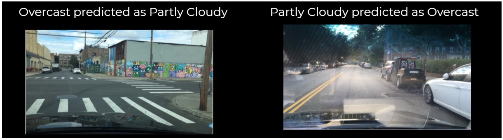
Figure 20 shows that overcast weather has been predicted as partly cloudy and vice versa. Both images do not have too much sky space displayed in the images. This challenges our classification model, making it hard to recognize the correct weather type.
Additionally, another constraint for this weather type classification model is the limitation of the night images. It is impossible for the model to detect whether it is clear, partly cloudy or overcast. Even for human eyes, we cannot tell the weather type from the night image. These are some things we may look into in the future to develop more advanced technology to classify the night images.
Intersection classification The classifier distinguished the three-way and four-way intersection by detecting the vertical and parallel road and capturing the indicator traffic signs, traffic lights and crosswalks. As shown in Table 16. The top five indicators with high importance scores derived from random forest models are right traffic light, no U-turn, front traffic light, right crosswalk, left traffic light. The direction of the traffic light and the location of the crosswalk are ideal indicators for classifying what types of intersection is within the images. For instance, a traffic light toward the left clearly tells us that there’s a drivable road on the left of the image; a crosswalk on the right side of the image indicates there’s a parallel road from the right- side; a one-way sign gives that there’s a road across the path we are currently on. With the indicators we detected from the images, we are able to classify what types of intersections we are approaching even though the image does not capture the entire intersection scene.
Table 16
Feature importance
| Features | Score | Features | Score | ||
| 5 | Front crosswalk | 0.207657 | 1 | One way point right | 0.049934 |
| 8 | Left traffic light | 0.129707 | 10 | No u turn | 0.039396 |
| 11 | Stop sign | 0.120155 | 0 | One way point left | 0.034375 |
| 9 | No left turn | 0.095648 | 6 | Front traffic light | 0.032561 |
| 7 | Right traffic light | 0.093700 | 2 | One way point front | 0.025884 |
| 12 | No right turn | 0.084474 | 3 | Left crosswalk | 0.017208 |
| 4 | Right crosswalk | 0.069300 |
The intersection indicators table of each street image is derived from the intersection indicators detection and road segmentation tasks. The first difficulty we encountered was at the phase of collecting suitable image data. We could not find a data source with a sufficient number of intersection images and the intersection indicators within the images. At the beginning, we used Google Map Street View API to generate the street images for the corresponding geolocations from the San Jose Intersection dataset. The dataset was released by the officials, providing more than 20,000 geolocations of the intersections in San Jose city. However, a large number of street images were taken near the neighborhood and had very few traffic signs, lights, and crosswalks. For intersections like, the detection model can only recognize that it is an intersection but will have a hard time classifying which types of intersections it is. As a result, we gave up using the official dataset and chose to create our own training set.
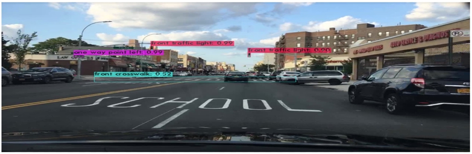
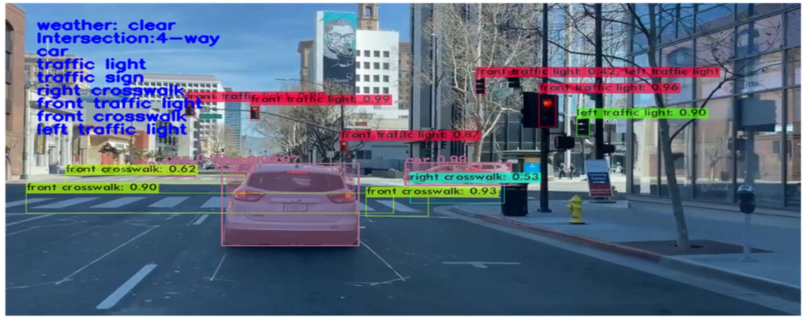
In addition to that, we also encountered a problem when labeling the crosswalks within the images. The bounding boxes can perfectly capture rectangular objects such as the traffic sign, or the traffic light, but when it comes to a crosswalk, a bounding box would also capture other objects overlapped with the crosswalk which interfere with our training. To solve the problem, we selected images with different types of crosswalks that were partially occluded to train with our detection model. Figure 21 shows a result from the improved model.
Fig. 21.
Detection result from the improved model.
7.2.System quality evaluation of model functions and performance
Regarding the model integration and development, we train and save the h5 files (a data file saved in the hierarchical data format), and use OpenCV and Flask packages to deliver the system result in a hybrid method. The model input may be various, thus we resize and set image with
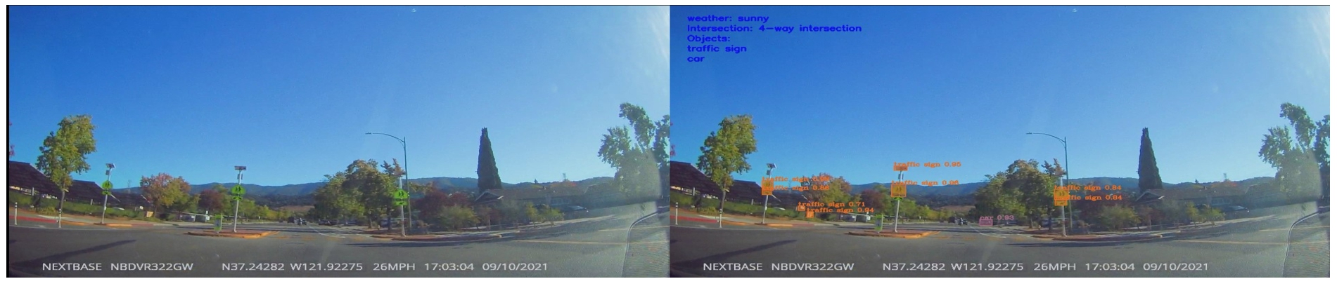
We use Flask and openCV to ensemble our models and display our image detection results for test images and our test videos, as well as our final intersection classification table for each intersection image. In Flask, we would display intersection images as two parts. In Fig. 22, the left side is the original image, while the right side is our model detection results. The image shows several pieces of information, such as weather conditions, object detection results, road detection results and the intersection type.
Fig. 22.
Model detection result.
We will merge our models results in OpenCV for the intersection detection for both test images and videos. The integrated stack system allows the user to input an image or a video and will output a demo result, as shown in Fig. 23.
Fig. 23.
Intersection detection demo.
7.3.Model support system
Google Colab Pro is an affordable managed service for building, training, deploying, and monitoring machine learning models. It provides decent capabilities and scalabilities for end-to-end machine learning or deep learning projects. Google Colab Pro will be used for data exploration and machine learning in this study. It meets intermediate computation requirements and GPU training (T4 or P100 GPU). Google Colab will be used for the data analysis process and model, including training, validation and testing datasets. In addition, Google Drive will be used for data storage (unlimited google drive storage if using edu email) and mounted and accessed through Colab scripts.
TensorFlow and Keras will be the tools for image preprocess and deep learning model development and implementation. TensorFlow is an open-sourced end-to-end platform and library for multiple machine learning tasks and it supports speed and parallelization using GPU, while Keras is a high-level neural network library that runs on top of TensorFlow. Both of them provide high-level APIs used for easily building and training models, but Keras is more user-friendly thanks to its built-in Python.
8.Conclusion
In this study, we used a large number of historical model training data and manually collected data from the street, including 100000 BDD100k object data, 3072 cityscapes weather data, 600 Mapillary intersection indicator detection data and 369 Mapillary intersection classification data. The COCO 2017 dataset was also used to train the model to recognize common targets on the road, including vehicles, people, animals, etc. We introduced 11 types of traffic target classifications, 71 types of coco target classifications, 2 Lane segmentation, 13 types of intersection indicators, 3 types of intersection classification and 6 types of weather classification. We propose a 2-stage integrated machine learning model to support city traffic context and transportation intersection classification. The performance of the model was evaluated using data collected in the field, and the results show that the 2-stage integrated model has higher recognition accuracy. This research has high potential application value for improving the safety and automation of autonomous driving systems in the future.
At this stage, we mainly use the video data collected by the camera installed in the front of the vehicle, but lack of research on the multi angle video data of the intersection. In future work, we will study the construction of a driverless stereo vision system using multi camera technology; Combine the information collected from multiple cameras to build a 3D representation of the surrounding world which will improve the depth estimation ability of the system and ensure the safety of vehicles and passengers.
Acknowledgements
Without the support of colleagues and friends around us, this paper could not be completed. The authors would like to take this opportunity to express their heartfelt thanks to all those who have helped them in the process of paper collaboration. First of all, they would like to thank many members of the research group for their joint efforts, which enabled them to obtain a wealth of experimental data. Secondly, they would like to thank other research team members who participated in the discussion in the process of this study. Their participation in the discussion provided them with more innovative ideas. Last but not least, they would like to thank their families for their support and understanding, which provided them with a comfortable atmosphere to complete this paper.
Conflict of interest
None to report.
References
[1] | A. & D. M., “Statistics on Intersection Accidents,” Sacramento Personal Injury Lawyer, AutoAccident.com. [Online]. Available https://www.autoaccident.com/statistics-on-intersection-accidents.html [Accessed: 27-Mar-2021]. |
[2] | U. Baumann, November. Classifying Road Intersections Using Transfer-Learning on a Deep Neural Network, 2018, 2018 21st International Conference on Intelligent Transportation (ITSC), https://ieeexplore.ieee.org/document/8569916. |
[3] | A. Bochkovskiy, C. Wang and H. Liao, (PDF) YOLOv4: Optimal Speed and Accuracy of Object Detection, ResearchGate, 23-Apr-2020. [Online]. Available https://www.researchgate.net/publication/340883401_YOLOv4_Optimal_Speed_and_Accuracy_of_Object_Detection. [Accessed: 27-Mar-2021]. |
[4] | A. Bochkovskiy, C. Wang and H. Liao, (PDF) YOLOv4: Optimal Speed and Accuracy of Object Detection, ResearchGate, 23-Apr-2020. [Online]. Available https://www.researchgate.net/publication/340883401_YOLOv4_Optimal_Speed_and_Accuracy_of_Object_Detection. [Accessed: 27-Mar-2021]. |
[5] | Clipchamp.What does fps Mean? Why You Need to Understand Video Frame Rate, https://clipchamp.com/pt-br/definition/what-does-fps-mean-frame-rates-explained/. |
[6] | Common objects in context. COCO. (n.d.). Retrieved December 18, 2021, from https://cocodataset.org/#download. |
[7] | Detection and classification of vehicles for traffic video, (n.d.). Retrieved December 18, 2021, from https://www.researchgate.net/publication/329111172_Detection_and_classification_of_vehicles_for_traffic_video_analytics. |
[8] | C. Ertler, J. Mislej, T. Ollmann, L. Porzi, G. Neuhold and Y. Kuang, The Mapillary Traffic Sign Dataset for Detection and Classification on a Global Scale. arXiv.org, 2020, https://arxiv.org/abs/1909.04422. |
[9] | D. Faggella, The Self-Driving Car Timeline – Predictions from the Top 11 Global Automakers, Emerj, 14-Mar-2020. [Online]. Available, Accessed: 27-Mar-2021, https://emerj.com/ai-adoption-timelines/self-driving-car-timeline-themselves-top-11-automakers/. |
[10] | B. Gringer, History of the Autonomous Car. TitleMax, 2020, https://www.titlemax.com/resources/history-of-the-autonomous-car/. |
[11] | K. He, G. Gkioxari, P. Dollár and R. Girshick, Mask R-CNN. arXiv.org (2017), Retrieved December 18, 2021, from https://arxiv.org/abs/1703.06870v2. |
[12] | X. Huang, P. Wang, X. Cheng, D. Zhou, Q. Geng and R. Yang, The apolloscape open dataset for autonomous driving and its Application, The ApolloScape Open Dataset for Autonomous Driving and its Application – arXiv Vanity, 2019, [Online]. Available https://www.arxiv-vanity.com/papers/1803.06184/. [Accessed: 18-Dec-2021]. |
[13] | R. Khandelwal, Evaluating performance of an object detection model, 2020, towardsdatascience, https://towardsdatascience.com/evaluating-performance-of-an-object-detection-model-137a349c517b. |
[14] | Y. Li, H. Wang, L. Dang, T. Nguyen, D. Han, A. Lee, I. Jang and H. Moon, A Deep Learning-Based Hybrid Framework for Object, IEEE Access 23–Oct–2020, [Online]. Available https://danglienminh.github.io/public/papers/access_yanfen_2020.pdf. [Accessed: 27-Mar-2021]. |
[15] | T.-Y. Lin, M. Maire, S. Belongie, L. Bourdev, R. Girshick, J. Hays, P. Perona, D. Ramanan, C.L. Zitnick and P. Dollár, Microsoft Coco: Common Objects in Context, arXiv.org, 2015. [Online]. Available https://arxiv.org/abs/1405.0312v3. [Accessed: 18-Dec-2021]. |
[16] | Y.P. Loh and C.S. Chan, Getting to know low-light images with the exclusively Dark Dataset, arXiv.org, 2018. [Online]. Available https://arxiv.org/abs/1805.11227. [Accessed: 18-Dec-2021]. |
[17] | Mapillary. (n.d.). Retrieved December 18, 2021, from https://www.mapillary.com/dataset/trafficsign. |
[18] | One account. all of google., Sign in – Google Accounts, [Online]. Available: https://waymo.com/open/about/. [Accessed: 18-Dec-2021]. |
[19] | H. Rajanathan, Berkeley Deep Drive Dataset – BDD100K. Medium (2021), Retrieved December 18, 2021, from https://hishoraj.medium.com/berkeley-deep-drive-dataset-bdd100k-b93bbfa10108. |
[20] | H. Rajanathan, Berkeley Deep Drive Dataset – BDD100K, Medium, 09-Jan-2021. [Online]. Available, Accessed: 18-Dec-2021, https://hishoraj.medium.com/berkeley-deep-drive-dataset-bdd100k-b93bbfa10108. |
[21] | S. Rao, How to Build a Data Pipeline for Autonomous Driving, NetApp Blog, 27-Jun-2019. [Online]. Available https://blog.netapp.com/how-to-build-a-data-pipeline-for-autonomous-driving/. [Accessed: 27-Mar-2021]. |
[22] | R. Rayaprolu, My ML development workflow, Medium, 07-Oct-2020. [Online]. Available https://medium.com/@helloraghuram/my-ml-development-workflow-550c19526719. [Accessed: 18-Dec-2021]. |
[23] | S. Sahoo, Residual blocks – Building blocks of ResNet, Toward Data Science (2018), https://towardsdatascience.com/residual-blocks-building-blocks-of-resnet-fd90ca15d6ec. |
[24] | D. Seita, BDD100K: A large-scale diverse driving video database, The Berkeley Artificial Intelligence Research Blog. Retrieved December 18 (n.d.), 2021, from https://bair.berkeley.edu/blog/2018/05/30/bdd/. |
[25] | P. Sharma, Imagenet competition results: 7 popular image classification models in Imagenet Challenge ILSVRC ompetition history MLK machine learning knowledge – * result of webvision 2020 challenge is released * the recent success of deep earning has shown that a deep architecture in conjunction with abundant., Imagenet Competition Results: 7 Popular Image Classification Models In Imagenet Challenge llsvrc Competition History Mlk Machine Learning Knowledge – * result of webvision 2020 challenge is released * the recent success of deep learning has shown that a deep architecture in conjunction with abundant., Jul-2020. [Online]. Available https://hdrawingcar.blogspot.com/2021/09/imagenet-competition-results-7-popular.html, Accessed: 18-Dec-2021. |
[26] | D. Tabernik and D. Skočaj, Deep Learning for Large-Scale Traffic-Sign Detection and Recognition, arXiv.org, 2019. [Online]. Available https://arxiv.org/abs/1904.00649. [Accessed: 27-Mar-2021]. |
[27] | D. Tabernik and D. Skočaj, Deep Learning for Large-Scale Traffic-Sign Detection and Recognition, arXiv.org, 2019. [Online]. Available https://arxiv.org/abs/1904.00649. [Accessed: 27-Mar-2021]. |
[28] | R.J. Tan, Breaking down mean average precision (map), Medium. (2020, July), https://towardsdatascience.com/breaking-down-mean-average-precision-map-ae462f623a52. |
[29] | P. Theodosis, L. Wilson and S. Cheng, EE368 Final Project: Road Sign Detection and Distance Estimation in Autonomous Car Application, [Online]. Available https://stacks.stanford.edu/file/druid:np318ty6250/Chen_Theodosis_Wilson_Stereo_Vision_in_Autonomous_Car_Application.pdf. [Accessed: 27-Mar-2021]. |
[30] | S.-H. Tsang, Review: Mask R-CNN (Instance Segmentation & Human Pose Estimation). Medium. Retrieved December 18, 2021, from https://medium.com/analytics-vidhya/review-mask-r-cnn-instance-segmentation-human-pose-estimation-61080a93bf4. |
[31] | P. Varma, 5 object detection evaluation metrics that data scientists should know, Analytics India Magazine. (2020, August), https://analyticsindiamag.com/5-object-detection-evaluation-metrics-that-data-scientists-should-know/. |
[32] | Z. Wan, J. Shen, J. Chuang, X. Xia, J. Garcia, J. Ma and Q.A. Chen, Too afraid to drive: Systematic discovery of semantic DoS vulnerability in autonomous driving planning under physical-world attacks, Network and Distributed Systems Security (NDSS) Symposium. ((2022) ). doi:10.48550/arxiv.2201.04610. |
[33] | G. Zaffiro, Smart Mobility: New roles for Telcos in the emergence of electric and autonomous vehicles, Jul-2019. [Online]. Available, Accessed:27-Mar-2021, https://www.researchgate.net/publication/334784348_Smart_Mobility_new_roles_for_Telcos_in_the_emergence_of_electric_and_autonomous_vehicles. |
[34] | P.S. Zaki, M.M. William, B.K. Soliman, K.G. Alexsan, K. Khalil and M. El-Moursy, Traffic Signs Detection and Recognition System using Deep Learning, [Online]. Available https://arxiv.org/abs/2003.03256 [Accessed: 27-Mar-2021]. |
[35] | X. Zhang, Simple understanding of mask RCNN. Medium. (2021), Retrieved December 18, 2021, from https://alittlepain833.medium.com/simple-understanding-of-mask-rcnn-134b5b330e95. |
[36] | Y. Zhang, J. Chu, L. Leng and J. Miao, Mask-refined R-CNN: A network for refining object details in instance segmentation (2020), MDPI. Retrieved, December 18, 2021, from https://www.mdpi.com/1424-8220/20/4/1010/htm. |
[37] | Z.-Q. Zhao, P. Zheng, S.-T. Xu and X. Wu, Object detection with deep learning: A review, IEEE Transactions on Neural Networks and Learning Systems 30: (11) ((2019) ), 3212–3232. doi:10.1109/TNNLS.2018.2876865. |


