
An optimal control model of the spread of the COVID-19 pandemic in Iraq: Deterministic and chance-constrained model
Abstract
Many studies have attempted to understand the true nature of COVID-19 and the factors influencing the spread of the virus. This paper investigates the possible effect the COVID-19 pandemic spreading in Iraq considering certain factors, that include isolation and weather. A mathematical model of cases representing inpatients, recovery, and mortality was used in formulating the control variable in this study to describe the spread of COVID-19 through changing weather conditions between 17th March and 15th May, 2020. Two models having deterministic and an uncertain number of daily cases were used in which the solution for the model using the Pontryagin maximum principle (PMP) was derived. Additionally, an optimal control model for isolation and each factor of the weather factors was also achieved. The results simulated the reality of such an event in that the cases increased by 118%, with an increase in the number of people staying outside of their house by 25%. Further, the wind speed and temperature had an inverse effect on the spread of COVID-19 by 1.28% and 0.23%, respectively. The possible effect of the weather factors with the uncertain number of cases was higher than the deterministic number of cases. Accordingly, the model developed in this study could be applied in other countries using the same factors or by introducing other factors.
1Introduction
The COVID-19 pandemic has resulted in a huge loss of human life and affected economies worldwide. Most nations have entered into a “lockdown” situation, isolating their economies from others in facing the virus and decrease the loss of human life. Several studies have investigated COVID-19 to understand the composition of the virus and determine the most suitable treatment. However, the danger of COVID-19 is represented by its spread without any clinical symptoms during the early stages of contracting the virus and long period incubation [19]. Chen et al. [2] compared two groups of patients; COVID-19 and SARS-CoV-2-negative, where it was revealed that COVID-19 patients suffered from high fever and cough more than SARS-CoV-2 patients. Procalcitonin (PCT) levels of SARS-CoV-2 patients (approximately 2 out of 5 patients) were shown to be higher compared to COVID-19 patients. Also, COVID-19 patients had lower creatinine levels compared with SARS-CoV-2 patients. In the case of those at a young age, the distinction between the two diseases can be diagnosed depending on the fever, cough, urea and creatinine levels, and parameters associated with routine blood workup. COVID-19, SARS and MERS have mostly similar pathological features [23]. However, the harm caused by COVID-19 may be caused by SARS-CoV-2 or through liver damage. Ai et al. [1] compared chest CT scans and reverse-transcription chain reaction to diagnose the virus in a sample of patients (1,014 patients) in China. Chest CT scans were shown to be highly sensitive in the diagnosis of the virus. X. Chen et al. [3] assessed the state of pregnant women, having a positive test for COVID-19, in which fever and cough were the main symptoms that were evident in the pregnant women without vertical transmission of the virus in late pregnancy. The World Health Organisation (WHO) confirmed the effect of COVID-19 on the mental health of human; especially children and the elderly [22].
The drug used for the treatment of malaria (Chloroquine phosphate) has found to be effective in the treatment of COVID-19 in some 100 patients through clinical trials conducted in hospitals across seven cities in China [6]. Lipsitch et al. [10] discussed the approach adopted in the treatment of an influenza pandemic (2009). While this approach may possibly be used in the treatment of Covid-19, it depends on many factors, such as existing surveillance systems. In a separate case, viral RNA samples were collected from survivors and people who had died to explore the factors that caused patients to die in a hospital setting by employing multivariable logistic regression [24].
In fact, several studies have formulated mathematical models to simulate actual cases of epidemics and pandemics around the world. In some studies, the optimal control model was widely used to determine the effect of vaccination and isolation. Lee et al. [9] clarified the effect of treatment and isolation on the control of fast transmitting diseases, such as influenza. In their study, they discussed isolation strategies having insufficient antiviral resources. Three models of optimal control, namely, vaccination, isolation and the mixed model of the SIR epidemic were investigated by Hansen and Day [8] to minimise the magnitude of the outbreak. Tuite et al. [18] explored control strategies that could aid in understanding the spreading processes associated with the cholera epidemic in Haiti to reduce the potential effects. Rodrigues et al. [15] discussed a dengue vaccine as a control variable with distinct levels and two methods of treatment. The first method was for paediatric patients, and the second method was for random mass vaccination. A comparison between a different scenario regarding tuberculosis epidemiological features was conducted by P. Rodrigues et al. [16], aiming to reduce total implementation costs and the number of infected cases. Also, regarding tuberculosis, Moualeu et al. [11] formulated a mathematical model that considers infection (diagnosed and undiagnosed), lost-sight, and latently infected aspects. Pang et al. [12] formulated a mathematical model that simulated the actual cases of measles transmission in the United States (US) for the period between 1951 and 1962 to determine the optimal strategy for vaccination. The spread of the Ebola virus in West Africa was investigated by Rachah and Torres [13, 14]. The first paper investigated the effect of different cases of vaccination on the virus spreading over time, while the second paper addressed in addition to vaccination, several strategies to reduce the number of infected and exposed individuals. In another study by Gao and Huang, they incorporated three controls as part of a strategy from among several initially developed strategies to minimise intervention costs and reduce the burden of tuberculosis [5].
The structure of this paper is organised into five sections. The first section, already discussed, provided a brief introduction and background information on COVID-19. Section 2 provides further information on the spread of COVID-19, followed by Section 3 that presents two models; the optimal control model and a model presenting an explicit solution using the Pontryagin maximum principle (PMP). The results and explanation of several models are presented and discussed in Section 4. Lastly, Section 5 presents the overall conclusions and recommendations for future research.
2The spread of COViD-19
In December 2019, the first cases of COVID-19 surfaced in Wuhan, Hubei, China [2]. Since then, four other Asian countries confirmed a further 282 cases of the virus on 20th January 2020, two cases in Thailand, one case Japan and South Korea, and the remaining number of cases were reported in China. All cases originated from Wuhan City [20].
After several months, the virus spread to other cities in China, and another 33 countries worldwide. On 24th February, the number of deaths reported in China amounted to 2,663, and 33 in other countries [1]. Towards the end of February 2020, the population in Europe and North America showed signs of the virus, albeit a different strain or foci of the virus, including countries in Asia, and the Middle East.
At the same time, the first case of COVID-19 was recorded in Africa and Latin America [21]. At the beginning of March 2020, more than 10,000 patients had died from the virus in 10 countries, including Iran, Italy, and South Korea [19]. A significant increase in the harm caused by the was in the Middle East was confirmed during the middle of March. As a result of the rapid spread of the virus, the WHO classified the COVID-19 epidemic as a global pandemic [21].
The first case of COVID-19 in Iraq appeared in the Najaf province, south of the capital Baghdad on 24th February 2020; an Iranian student studying Islamic science in Najaf. Many Iraqi people travel to Iran to visit many of the holy shrines and enjoy tourist attractions. It was believed that the virus originated from Iran. On 26th February, four new cases were reported with the number increasing to 13 on 1st March, before reporting 93 further cases in the middle of March with nine deaths.
3Optimal control model
This section presents two models having a known and uncertain number of new daily cases; the deterministic model and the chance-constrained model, respectively.
3.1Deterministic model
Optimal control for optimization is defined by:
(1)
Subject to the state equations of cases, inpatients, recovered cases and death:
(2)
(3)
(4)
(5)
where,
y(t): The control variable.
C(t): Percent of confirmed cases.
I(t): Percent of inpatients.
R(t): Percent of recovered cases.
D(t): Percent of death cases.
β(t): Percent of the new cases to the inpatient cases.
μ(t): Percent of the recover cases to the inpatient cases.
ΔC(t) = C(t)-C(t-1)
Equation (2) signifies the total number of cases that increased based on new cases daily. The total number of inpatients increases by the addition of new cases and decreases by the number of recovery and deaths each day (Equation 3). Equations (4 & 5) represent the total number of recovered patients and deaths, respectively. The control variable represents the percentage of isolation or each weather factor.
By using the PMP, determining the solution of the optimal control model can be achieved. The Lagrangian function is expressed as follows [17]:
(6)
A Hamiltonian function is expressed as:
(7)
Substituting Equation (7) into Equation (6), gives:
(8)
Deriving Equation (8) concerning C (t) , I (t) , R (t) , D (t), separately, gives:
(9)
(10)
(11)
(12)
By rearranging Equations (9–12), we can determine the adjoint equations as:
(13)
(14)
(15)
(16)
From Equations (13 - 14), we get:
(17)
(18)
Rearranging Equation (13), yields:
(19)
By substituting Equation (19) into Equation (2), it yields:
(20)
From Equation (20), we can determine the total number of cases over time as follows:
(21)
By substituting Equation (19) into Equation (3), it yields:
(22)
From Equation (22), we then get:
(23)
Then, substituting Equation (21) into Equation (23), it yields:
(24)
Equation (24) represents the total number of inpatients over time. We can determine the total number of recovered cases over time by substituting Equation (24) into Equation (4) as follows:
(25)
Substituting Equation (24) into Equation (5) yields the total number of death cases over time as follows:
(26)
Thus, the value of the control variable is as follows:
(27)
From Equation (27), y (t) = -1 means:
(28)
(29)
(30)
Initially the value of the control variable is zero, which means the model represents the actual cases registered in Iraq with the real percentage of new cases, recovered, and deaths as follows:
(31)
Next, by introducing the effect of wind (for example): changing the value of the control variable and cases depending on the wind degree (W) and transition matrix (φ) (see Appendix) we get:
(32)
(33)
(34)
Where ABS = absolute value.
The elements of the transition matrix can be calculated as follows (for example, humidity):
(35)
Where
Finally, the next tasks include incorporating the value of the control variable into an optimal control model to obtain the solution. The solution of the optimal control model relies on Equations (15–18, 21, 24–26). The solution is found by using the goal seek function in Microsoft Excel with λ(T) = 0. Hence, achieving the condition λ(T) = 0 by changing the value of λ(0).
3.2Chance-constrained model
The number of new cases reported in Iraq depends on the number of samples tested. Therefore, the actual cases may be is greater than those recorded cases. In this model, the number of new cases is uncertain given by the equation representing chance-constrained:
(36)
Where α takes values between zero and one (1) and NC is a random variable (new cases).
In determining the solution, chance-constrained must be converted to deterministic constrained. Here, the value of α is equal to zero or one (1) representing an extremely risky or extremely conservative attitude, respectively. The minimum acceptable to achieve the constraint is α, while (1 - α) is the maximum acceptable risks [7].
If NC is a random variable that adheres to a normal distribution with mean
(37)
Where ∅ is the cumulative distribution function (CDF) of the standard normal distribution.
The number of daily cases can be found from Eq. (37) with the initial value of cases C (0). To determine the effect of the weather factors, we apply the deterministic model (Equations 1–5) with the daily cases of chance-constrained (Equation 37).
4Numerical results
Table 1 (see Appendix) shows the number of COVID-19 cases and degrees of temperature, humidity, wind and pressure from 17th March to 15th May. First, we determine the values of (β,μ,N) by using Equation (31) to fit the actual cases reported in Table (1) with a zero (0) value of the control variable (see Table 2 in the Appendix).
Next, we change the control variable value to determine the results that represent the effect of isolation and weather.
The effect of isolation is determined by presenting the value of the control variable given below:
Figure (1) shows the effect of isolation on the results, with the actual cases (A.C.), increased cases (I.C.), and decreased cases (D.C.). From Fig. (1), we can conclude that the number of cases increases, due to increase in the number of people that did not commit to staying at home (y(t) = 0.25), and vice versa.
Fig. 1
The effect of isolation.
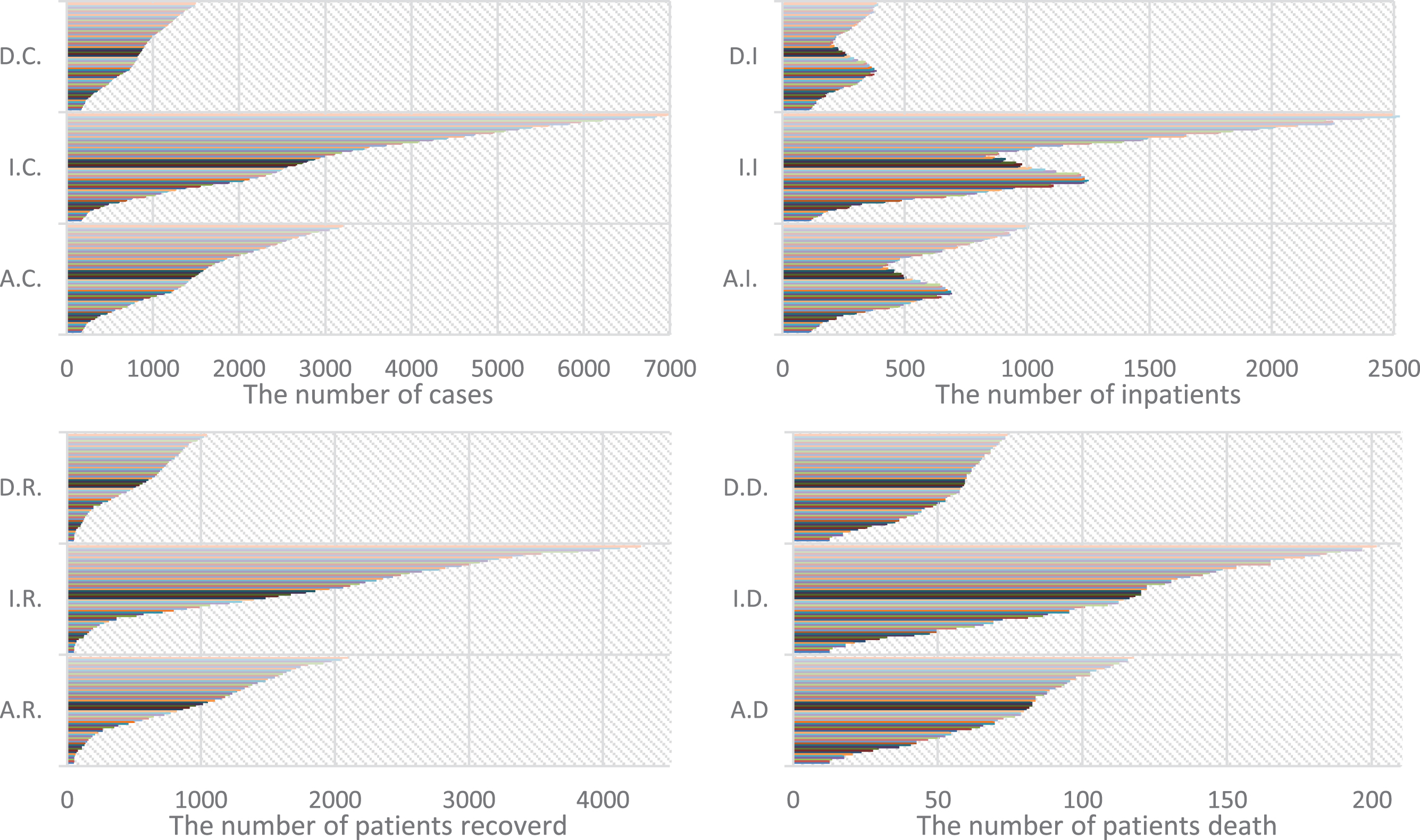
The increase in the per cent of people that did not commit to staying at home by 25% led to an increase in the number of COVID-19 cases by 118%, while, the proportion of COVID-19 cases decreased by 53.4% with an increase in the number of citizens staying at home by 25%. The numbers of inpatients (A.I, I.I, D.I), recoverd (A.R, I.R, D.R) and deaths (A.D, I.D, D.D) follow the number of cases.
According to the WHO, symptoms of infection first appear between 2 and 14 days, usually 5 days. In this case, we take the weather for the last 5 days (see Table 3 in the Appendix). We can then find the transition matrix for each factor of the weather (see Tables 4–7 in the Appendix) from Table (3). The values of the main diagonal are zero (0) (without effect) and the other values are negative (cases decrease) and positive (cases increase). The values of the transition matrix represent an increase (or decrease) of COVID-19 cases with an increase (or decrease) for every one (1) degree of the weather.
From Equations (32–34), and Table (4), we can determine the value of the control variable, according to the effect of humidity. Figure (2) shows the possible effect of humidity on the number of new cases.
Fig. 2
Numbers of new cases with and without the effect of humidity.

The white colour represents the number of new cases without the effect of humidityt, which means the default number. Meanwhile, the actual number of cases, affected by the humidity, is represented by gray colour. The explanation for Fig. (2) is as follows:
Two colours having the same value signifies no change in humidity, thus having no effect.
The white colour higher than the gray colour means humidity increases, while for new cases is decreases.
The other case means a decrease in humidity and an increase in new cases.
Similarly, we determine the possible effect of other weather factors, as can be seen in Figs. (3–5):
Fig. 3
Numbers of new cases with and without the effect of temperature.
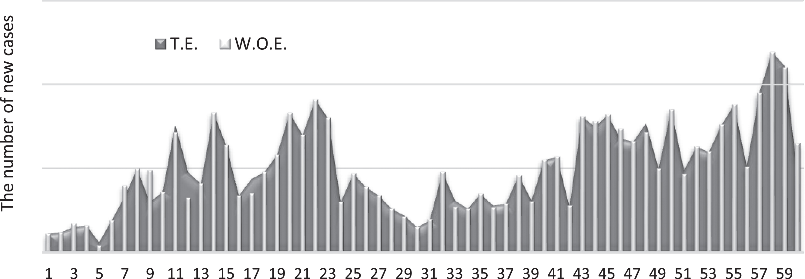
Fig. 4
Numbers of new cases with and without the effect of wind.
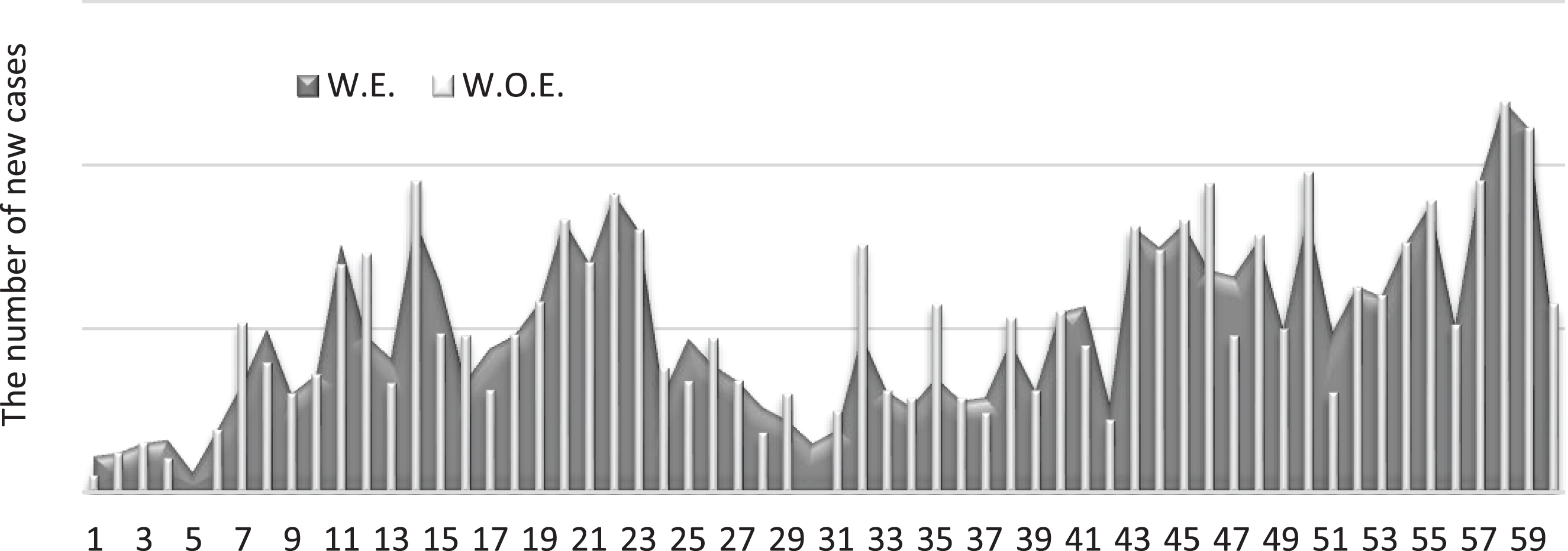
Fig. 5
Numbers of new cases with and without the effect of pressure.
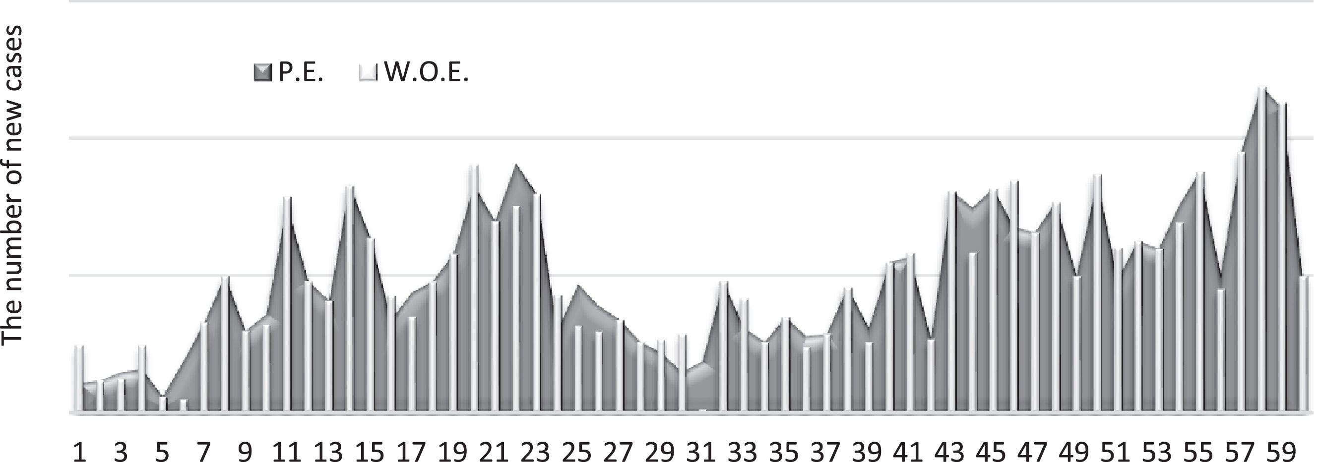
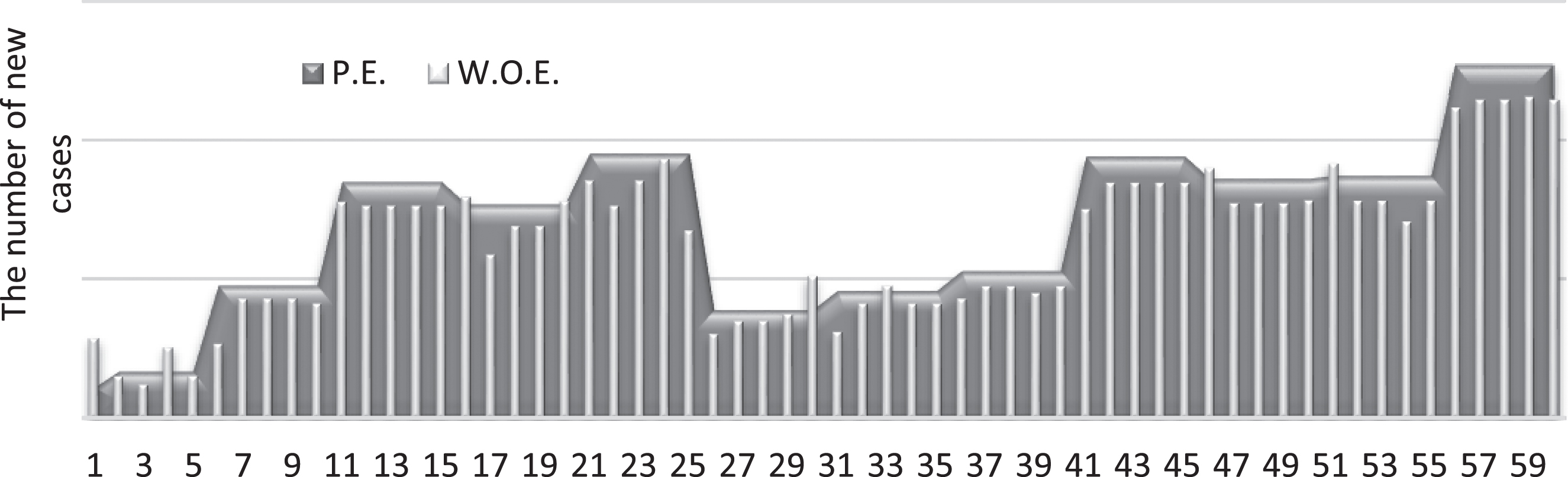
As evident in Figs. (2–5), the wind shows as having the highest effect on the number of new COVID-19 cases. Figure (6) shows the possible effect of the weather factors at the end of period.
Fig. 6
Weather factors and effect.
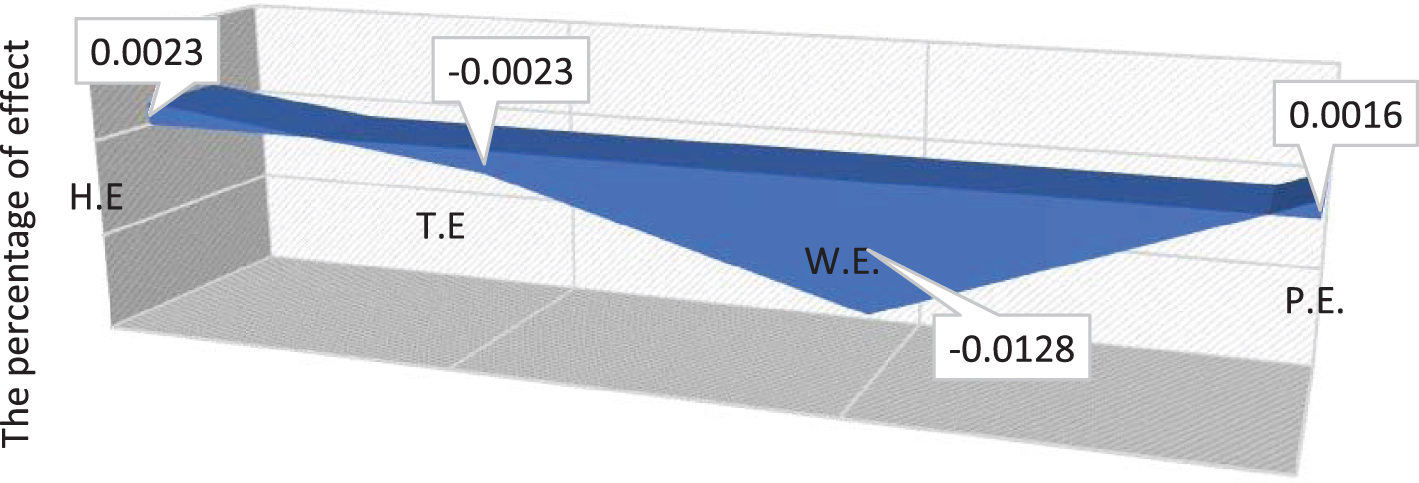
Figure (6) shows the possible effect of weather on the number of new COVID-19 cases. Wind (W.E) and pressure (P.E.) represent the highest and lowest effect, respectively. However, the effect of isolation (see Fig. 1) is more important compared to the weather factors. Figure (7) shows the results at the end of the period without the effect of the weather.
Fig. 7
The results of optimal control model with different values of the control variable.
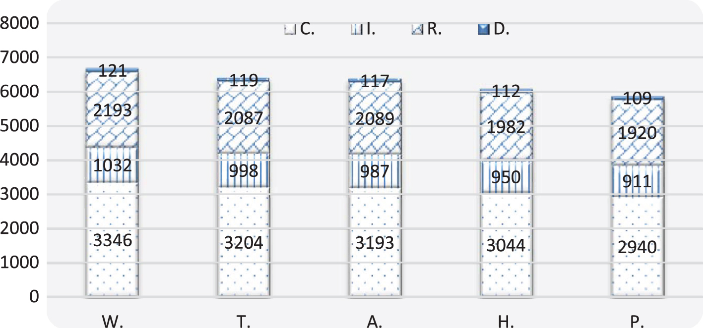
From Fig. (7), it can be seen that the increase in wind speed (W) and temperature (T) has led to a decrease in the number of COVID-19 cases. For example, the number of cases is 3,346 and 3,204 without the possible effect of both wind and temperature, respectively. Whereas the number of cases slightly increased with an increase in humidity (H) and pressure (P) compared to the number of actual cases (A).
For the chance-constraint model, the β value is changed according to Eq. (36). At first, we divide the study period into 12 sub-periods with 5 days for each sub-period. Next, a normality test of observations of the sub-periods is conducted, in which all sub-periods adhere to a normal distribution (see Table 8). Eq. (36) is then applied to determine the daily cases with α = 0.90 and ∅-1 (α) = 1.28. Finally, the same steps of the deterministic model are used to find the solution. From Equations (32–34), and Table (9), we can find the value of the control variable and the possible effect of the weather factors, as shown in Figs. (8–11).
Fig. 8
Number of new cases with and without the effect of humidity (chance-constrained).

Fig. 9
Number of new cases with and without the wind effect (chance-constrained).
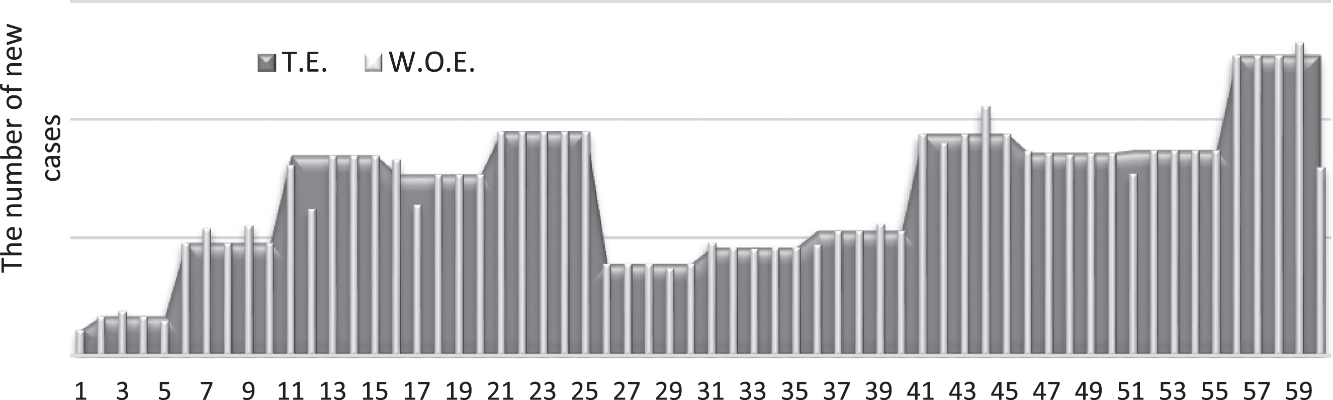
Fig. 10
Number of new cases with and without the pressure effect (chance-constrained).
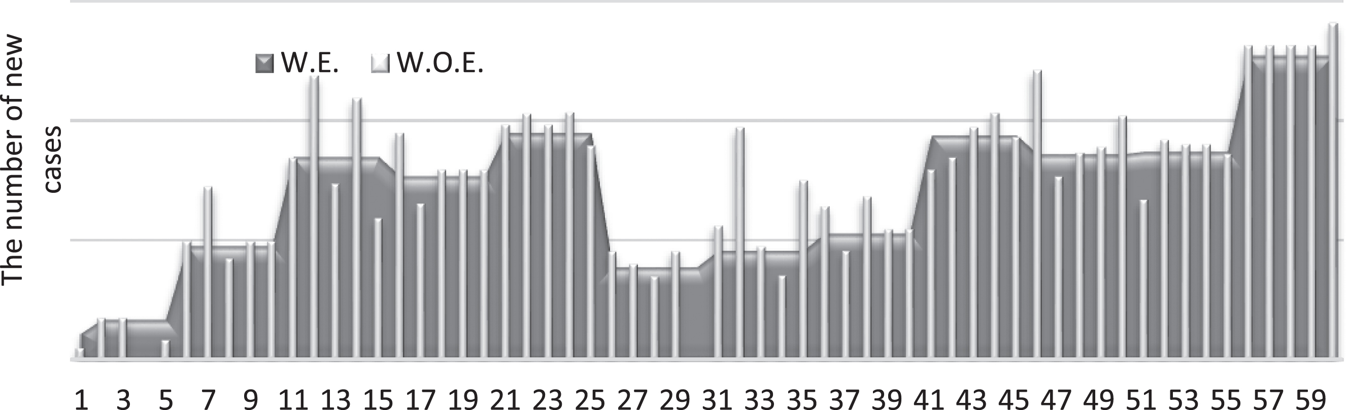
Fig. 11
Number of new cases with and without the pressure effect (chance-constrained).
By observing Figs. (8–11), the pressure signifies the highest effect on the number of new COVID-19 cases. Whereas, the wind represents the second-highest effect, but with an inverse relation to COVID-19 cases. Figure (12) below illustrates the possible proportional effect of the weather factors at the end of the period.
Fig. 12
Proportion, (as a percentage) due to the effect of weather (chance-constrained).
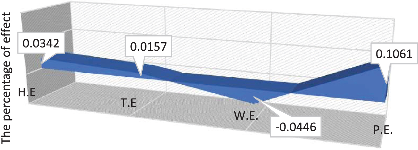
From observing Fig. (12), we can see that the pressure (P.E) and temperature (T.E.) represent the highest and lowest effect, respectively. The effect of the weather in the chance-constrained model is higher than the deterministic model because the increase in the number of COVID-19 cases is according to the chance-constrained model.
5Conclusion
In this paper, the possible effect of both weather factors and isolation on the spread of COVID-19 in the context of Iraq was investigated, finding that temperature, humidity, wind, and pressure had a noticeable effect on the spread of the virus. An optimal control model was developed to describe the spread of COVID-19 cases, Deterministic and chance-constrained models were also developed, and the solution of the model using the PMP was also derived. The transition matrix for each of the factor factors was addressed.
Initially, a control variable y(t) representing the percentage of isolation and weather factors was determined. The zero value of the control variable represented the actual data of COVID-19 cases in Iraq, while the optimal solution was determined with y = –1. Next, was determining the value of the control variable with respect to five models, before finally, clarifying the possible effect of isolation and the weather factors on the spread of COVID-19.
Accordingly, it was shown that isolation was significant in containing COVID-19 from contagion. On the other hand, the number of cases increased by 118% attributed to an increase in the number of people who ignored the need to stay at home, which rose by 25%. In contrast, the cases reduced by 53.4% for the opposite case where people stayed at home.
These statistics also support the nature of the virus in reality since it is highly contagious, spreading from one person to many. Weather factors also had a noticeable effect on the spread of COVID-19, though lower than self-isolation. Likewise, both wind speed and temperature had the highest effect compared with other weather factors. Further, the wind speed and temperature had an inverse effect on the spread of COVID-19 by 1.28% and 0.23%, respectively, while a positive relationship with humidity and pressure. Humidity and temperature had a similar effect but opposingly. Moreover, increasing the number of daily cases of COVID-19, according to the chance-constrained model, weather factors had a greater effect.
Accordingly, the model developed in this study could be applied in other countries using the same factors or by introducing other factors, such as communication, transportation, and payment.
Appendices
Appendix
Table 1
The number of COVID-19 cases and weather degrees in Iraq
| Date | Cases | Recover | Death | New Cases | Temp. | Wind | Humid. | Pres. |
| 17 March | 165 | 43 | 12 | 11 | 26 | 7 | 40 | 1015 |
| 18 | 177 | 49 | 12 | 12 | 22 | 13 | 39 | 1010 |
| 19 | 192 | 49 | 13 | 15 | 18 | 7 | 57 | 1016 |
| 20 | 208 | 49 | 17 | 16 | 23 | 9 | 32 | 1014 |
| 21 | 214 | 52 | 17 | 6 | 22 | 7 | 45 | 1006 |
| 22 | 233 | 57 | 20 | 19 | 17 | 2 | 52 | 1011 |
| 23 | 266 | 62 | 23 | 33 | 20 | 9 | 46 | 1015 |
| 24 | 316 | 75 | 27 | 50 | 24 | 4 | 34 | 1014 |
| 25 | 346 | 103 | 29 | 30 | 27 | 13 | 29 | 1009 |
| 26 | 382 | 105 | 36 | 36 | 28 | 20 | 30 | 1010 |
| 27 | 458 | 122 | 40 | 76 | 24 | 11 | 40 | 1014 |
| 28 | 506 | 131 | 42 | 48 | 24 | 7 | 46 | 1009 |
| 29 | 547 | 143 | 42 | 41 | 22 | 7 | 50 | 1014 |
| 30 | 630 | 152 | 46 | 83 | 23 | 9 | 33 | 1012 |
| 31 | 694 | 170 | 50 | 64 | 26 | 4 | 26 | 1017 |
| 1 April | 728 | 182 | 52 | 34 | 28 | 26 | 29 | 1007 |
| 2 | 772 | 202 | 54 | 44 | 26 | 9 | 28 | 1012 |
| 3 | 820 | 226 | 54 | 48 | 25 | 4 | 33 | 1016 |
| 4 | 878 | 259 | 56 | 58 | 25 | 9 | 37 | 1018 |
| 5 | 961 | 259 | 61 | 83 | 26 | 4 | 29 | 1021 |
| 6 | 1031 | 344 | 64 | 70 | 29 | 9 | 30 | 1014 |
| 7 | 1122 | 373 | 65 | 91 | 26 | 9 | 37 | 1012 |
| 8 | 1202 | 452 | 69 | 80 | 30 | 7 | 27 | 1010 |
| 9 | 1232 | 496 | 69 | 30 | 26 | 4 | 54 | 1006 |
| 10 | 1279 | 550 | 70 | 47 | 25 | 7 | 35 | 1008 |
| 11 | 1318 | 601 | 72 | 39 | 25 | 9 | 30 | 1012 |
| 12 | 1352 | 640 | 76 | 34 | 26 | 6 | 29 | 1016 |
| 13 | 1378 | 717 | 78 | 26 | 27 | 10 | 33 | 1017 |
| 14 | 1400 | 766 | 78 | 22 | 27 | 13 | 15 | 1017 |
| 15 | 1415 | 812 | 79 | 15 | 29 | 17 | 11 | 1016 |
| 16 | 1434 | 856 | 80 | 19 | 30 | 2 | 17 | 1013 |
| 17 | 1482 | 906 | 81 | 48 | 32 | 7 | 14 | 1011 |
| 18 | 1513 | 953 | 82 | 31 | 31 | 4 | 21 | 1011 |
| 19 | 1539 | 1009 | 82 | 26 | 28 | 7 | 29 | 1015 |
| 20 | 1574 | 1043 | 82 | 35 | 32 | 4 | 21 | 1013 |
| 21 | 1602 | 1096 | 83 | 28 | 33 | 4 | 20 | 1012 |
| 22 | 1631 | 1146 | 83 | 29 | 33 | 4 | 25 | 1010 |
| 23 | 1677 | 1171 | 83 | 46 | 37 | 6 | 18 | 1004 |
| 24 | 1708 | 1204 | 86 | 31 | 29 | 6 | 29 | 1008 |
| 25 | 1763 | 1224 | 87 | 55 | 32 | 13 | 21 | 1001 |
| 26 | 1820 | 1263 | 87 | 57 | 26 | 13 | 33 | 1008 |
| 27 | 1847 | 1286 | 88 | 27 | 28 | 6 | 23 | 1013 |
| 28 | 1928 | 1319 | 90 | 81 | 31 | 9 | 17 | 1011 |
| 29 | 2003 | 1346 | 92 | 75 | 24 | 4 | 29 | 1008 |
| 30 | 2085 | 1375 | 93 | 82 | 24 | 6 | 40 | 1009 |
| 1 May | 2153 | 1414 | 94 | 68 | 31 | 6 | 26 | 1014 |
| 2 | 2219 | 1473 | 95 | 66 | 36 | 2 | 16 | 1011 |
| 3 | 2296 | 1490 | 97 | 77 | 33 | 11 | 20 | 1013 |
| 4 | 2346 | 1544 | 97 | 50 | 26 | 15 | 45 | 1011 |
| 5 | 2431 | 1571 | 102 | 85 | 29 | 11 | 21 | 1018 |
| 6 | 2480 | 1602 | 102 | 49 | 31 | 7 | 20 | 1016 |
| 7 | 2543 | 1626 | 102 | 63 | 37 | 4 | 13 | 1009 |
| 8 | 2603 | 1661 | 104 | 60 | 29 | 9 | 33 | 1008 |
| 9 | 2679 | 1702 | 107 | 76 | 29 | 13 | 20 | 1008 |
| 10 | 2767 | 1734 | 109 | 88 | 29 | 9 | 21 | 1010 |
| 11 | 2818 | 1790 | 110 | 51 | 32 | 6 | 17 | 1015 |
| 12 | 2913 | 1903 | 112 | 95 | 35 | 4 | 13 | 1013 |
| 13 | 3032 | 1966 | 115 | 119 | 39 | 9 | 8 | 1011 |
| 14 | 3143 | 2028 | 115 | 111 | 40 | 11 | 10 | 1009 |
| 15 | 3193 | 2089 | 117 | 50 | 41 | 15 | 10 | 1008 |
The ministry of health/ Iraq.
https://www.timeanddate.com/weather/iraq/baghdad/historic?month=4&year=2020.
Table 2
The values of the model parameters
| Date | β | μ |
|
| 17 March | 0.066667 | 0.100000 | 0.009091 |
| 18 | 0.067797 | 0.051724 | 0.000000 |
| 19 | 0.078125 | 0.000000 | 0.007692 |
| 20 | 0.076923 | 0.000000 | 0.028169 |
| 21 | 0.028037 | 0.020690 | 0.000000 |
| 22 | 0.081545 | 0.032051 | 0.019231 |
| 23 | 0.124060 | 0.027624 | 0.016575 |
| 24 | 0.158228 | 0.060748 | 0.018692 |
| 25 | 0.086705 | 0.130841 | 0.009346 |
| 26 | 0.094241 | 0.008299 | 0.029046 |
| 27 | 0.165939 | 0.057432 | 0.013514 |
| 28 | 0.094862 | 0.027027 | 0.006006 |
| 29 | 0.074954 | 0.033149 | 0.000000 |
| 30 | 0.131746 | 0.020833 | 0.009259 |
| 31 | 0.092219 | 0.037975 | 0.008439 |
| 1 April | 0.046703 | 0.024291 | 0.004049 |
| 2 | 0.056995 | 0.038760 | 0.003876 |
| 3 | 0.058537 | 0.044444 | 0.000000 |
| 4 | 0.066059 | 0.058615 | 0.003552 |
| 5 | 0.086368 | 0.000000 | 0.007800 |
| 6 | 0.067895 | 0.136437 | 0.004815 |
| 7 | 0.081105 | 0.042398 | 0.001462 |
| 8 | 0.066556 | 0.116006 | 0.005874 |
| 9 | 0.024351 | 0.065967 | 0.000000 |
| 10 | 0.036747 | 0.081942 | 0.001517 |
| 11 | 0.029590 | 0.079070 | 0.003101 |
| 12 | 0.025148 | 0.061321 | 0.006289 |
| 13 | 0.018868 | 0.132075 | 0.003431 |
| 14 | 0.015714 | 0.088129 | 0.000000 |
| 15 | 0.010601 | 0.087786 | 0.001908 |
| 16 | 0.013250 | 0.088353 | 0.002008 |
| 17 | 0.032389 | 0.101010 | 0.002020 |
| 18 | 0.020489 | 0.098326 | 0.002092 |
| 19 | 0.016894 | 0.125000 | 0.000000 |
| 20 | 0.022236 | 0.075724 | 0.000000 |
| 21 | 0.0174781 | 0.125295 | 0.002364 |
| 22 | 0.0177805 | 0.124378 | 0 |
| 23 | 0.0274299 | 0.059101 | 0 |
| 24 | 0.0181498 | 0.078947 | 0.007177 |
| 25 | 0.0311968 | 0.044247 | 0.002212 |
| 26 | 0.0313186 | 0.082978 | 0 |
| 27 | 0.0146183 | 0.048625 | 0.002114 |
| 28 | 0.0420124 | 0.063583 | 0.003853 |
| 29 | 0.0374438 | 0.047787 | 0.003539 |
| 30 | 0.0393285 | 0.047001 | 0.001620 |
| 1 May | 0.0315838 | 0.060465 | 0.001550 |
| 2 | 0.0297431 | 0.090629 | 0.001536 |
| 3 | 0.0335365 | 0.023977 | 0.002820 |
| 4 | 0.0213128 | 0.076595 | 0 |
| 5 | 0.0349650 | 0.035620 | 0.006596 |
| 6 | 0.0197580 | 0.039948 | 0 |
| 7 | 0.0247738 | 0.029447 | 0 |
| 8 | 0.0230503 | 0.041766 | 0.002386 |
| 9 | 0.0283687 | 0.047126 | 0.003448 |
| 10 | 0.0318033 | 0.034632 | 0.002164 |
| 11 | 0.0180979 | 0.061002 | 0.001089 |
| 12 | 0.0326124 | 0.125835 | 0.002227 |
| 13 | 0.0392480 | 0.066246 | 0.003154 |
| 14 | 0.035316 | 0.062 | 0 |
| 15 | 0.015659 | 0.061803 | 0.002026 |
Table 3
The average of COVID-19 cases, according to humidity, temperature, wind and pressure
| Humid. |
| Temp. |
| Wind |
| Pres. |
|
| 56–75 | 50 | 91–100 | 55 | 21–25 | 40 | 5026–5035 | 55 |
| 76–100 | 51 | 101–110 | 23 | 26–30 | 52 | 5036–5045 | 79 |
| 101–125 | 60 | 111–120 | 31 | 31–35 | 54 | 5046–5055 | 57 |
| 126–150 | 56 | 121–130 | 53 | 36–40 | 41 | 5056–5065 | 50 |
| 151–175 | 67 | 131–140 | 51 | 41–45 | 59 | 5066–5075 | 38 |
| 176–200 | 48 | 141–150 | 58 | 46–50 | 61 | 5076–5085 | 60 |
| 201–225 | 28 | 151–160 | 62 | 51–55 | 53 | ||
| 226–250 | 22 | 161–170 | 64 | 56–60 | 34 | ||
| 251–275 | 12 | 171–180 | 50 |
Table 4
The transition matrix of the number of COVID-19 cases, according to humidity
| State | 75 | 100 | 125 | 150 | 175 | 200 | 225 | 250 | 275 |
| 75 | 0.000 | 0.030 | 0.208 | 0.084 | 0.170 | –0.013 | –0.147 | –0.160 | –0.190 |
| 100 | –0.030 | 0.000 | 0.386 | 0.111 | 0.217 | –0.024 | –0.182 | –0.192 | –0.221 |
| 125 | –0.208 | –0.386 | 0.000 | –0.164 | 0.132 | –0.161 | –0.324 | –0.307 | –0.323 |
| 150 | –0.084 | –0.111 | 0.164 | 0.000 | 0.428 | –0.159 | –0.377 | –0.343 | –0.354 |
| 175 | –0.170 | –0.217 | –0.132 | –0.428 | 0.000 | –0.745 | –0.780 | –0.600 | –0.550 |
| 200 | 0.013 | 0.024 | 0.161 | 0.159 | 0.745 | 0.000 | –0.815 | –0.527 | –0.485 |
| 225 | 0.147 | 0.182 | 0.324 | 0.377 | 0.780 | 0.815 | 0.000 | –0.240 | –0.320 |
| 250 | 0.160 | 0.192 | 0.307 | 0.343 | 0.600 | 0.527 | 0.240 | 0.000 | –0.400 |
| 275 | 0.190 | 0.221 | 0.323 | 0.354 | 0.550 | 0.485 | 0.320 | 0.400 | 0.000 |
Table 5
The transition matrix of the number of COVID-19 cases, according to temperature
| State | 100 | 110 | 120 | 130 | 140 | 150 | 160 | 170 | 180 |
| 100 | 0.000 | –3.167 | –1.200 | –0.070 | –0.107 | 0.053 | 0.652 | 0.464 | –0.036 |
| 110 | 3.167 | 0.000 | 0.767 | 2.958 | 1.370 | 1.143 | 1.143 | 0.803 | 0.444 |
| 120 | 1.200 | –0.767 | 0.000 | 2.191 | 0.986 | 0.888 | 0.787 | 0.650 | 0.317 |
| 130 | 0.070 | –2.958 | –2.191 | 0.000 | –0.218 | 0.236 | 0.318 | 0.265 | –0.058 |
| 140 | 0.107 | –1.370 | –0.986 | 0.218 | 0.000 | 0.690 | 0.587 | 0.426 | –0.018 |
| 150 | –0.053 | –1.143 | –0.888 | –0.236 | –0.690 | 0.000 | 0.484 | 0.294 | –0.254 |
| 160 | –0.652 | –0.978 | –0.787 | –0.318 | –0.587 | –0.484 | 0.000 | 0.104 | –0.623 |
| 170 | –0.464 | –0.803 | –0.650 | –0.265 | –0.426 | –0.294 | –0.104 | 0.000 | –1.350 |
| 180 | 0.036 | –0.444 | –0.317 | 0.058 | 0.018 | 0.254 | 0.623 | 1.350 | 0.000 |
Table 6
The transition matrix of the number of COVID-19 cases, according to wind
| State | 25 | 30 | 35 | 40 | 45 | 50 | 55 | 60 |
| 25 | 0.000 | 2.400 | 1.367 | 0.036 | 0.958 | 0.851 | 0.446 | –0.177 |
| 30 | –2.400 | 0.000 | 0.333 | –1.145 | 0.477 | 0.464 | 0.055 | –0.607 |
| 35 | –1.367 | –0.333 | 0.000 | –2.624 | 0.549 | 0.508 | –0.015 | –0.795 |
| 40 | –0.036 | 1.145 | 2.624 | 0.000 | 3.722 | 2.074 | 0.855 | –0.337 |
| 45 | –0.958 | –0.477 | –0.549 | –3.722 | 0.000 | 0.426 | –0.578 | –1.690 |
| 50 | –0.851 | –0.464 | –0.508 | –2.074 | –0.426 | 0.000 | –1.582 | –2.749 |
| 55 | –0.446 | –0.055 | 0.015 | –0.855 | 0.578 | 1.582 | 0.000 | –3.915 |
| 60 | 0.177 | 0.607 | 0.795 | 0.337 | 1.690 | 2.749 | 3.915 | 0.000 |
Table 7
The transition matrix of the number of COVID-19 cases, according to pressure
| State | 5035 | 5045 | 5055 | 5065 | 5075 | 5085 |
| 5035 | 0.000 | 2.350 | 0.123 | –0.158 | –0.436 | 0.090 |
| 5045 | –2.350 | 0.000 | –2.104 | –1.413 | –1.364 | –0.475 |
| 5055 | –0.123 | 2.104 | 0.000 | –0.721 | –0.995 | 0.068 |
| 5065 | 0.158 | 1.413 | 0.721 | 0.000 | –1.268 | 0.463 |
| 5075 | 0.436 | 1.364 | 0.995 | 1.268 | 0.000 | 2.193 |
| 5085 | –0.090 | 0.475 | –0.068 | –0.463 | –2.193 | 0.000 |
Table 8
The number of cases, according to chance-constrained model
| Date | Cases | β | Mean | S.D. |
| 17 March | 165 | 0.066667 | 12.00 | 3.94 |
| 18 | 182 | 0.093407 | ||
| 19 | 199 | 0.085427 | ||
| 20 | 216 | 0.078704 | ||
| 21 | 233 | 0.072961 | ||
| 22 | 281 | 0.170819 | 33.60 | 11.19 |
| 23 | 329 | 0.145897 | ||
| 24 | 377 | 0.127321 | ||
| 25 | 425 | 0.112941 | ||
| 26 | 473 | 0.10148 | ||
| 27 | 558 | 0.15233 | 62.40 | 17.87 |
| 28 | 643 | 0.132193 | ||
| 29 | 728 | 0.116758 | ||
| 30 | 813 | 0.104551 | ||
| 31 | 898 | 0.094655 | ||
| 1 April | 975 | 0.078974 | 53.40 | 18.65 |
| 2 | 1052 | 0.073194 | ||
| 3 | 1129 | 0.068202 | ||
| 4 | 1206 | 0.063847 | ||
| 5 | 1283 | 0.060016 | ||
| 6 | 1378 | 0.06894 | 63.60 | 24.83 |
| 7 | 1473 | 0.064494 | ||
| 8 | 1568 | 0.060587 | ||
| 9 | 1663 | 0.057126 | ||
| 10 | 1758 | 0.054039 | ||
| 11 | 1797 | 0.021703 | 27.20 | 9.52 |
| 12 | 1836 | 0.021242 | ||
| 13 | 1875 | 0.0208 | ||
| 14 | 1914 | 0.020376 | ||
| 15 | 1953 | 0.019969 | ||
| 16 | 1999 | 0.023012 | 31.80 | 10.85 |
| 17 | 2045 | 0.022494 | ||
| 18 | 2091 | 0.021999 | ||
| 19 | 2137 | 0.021526 | ||
| 20 | 2183 | 0.021072 | ||
| 21 | 2236 | 0.023703 | 37.80 | 12.07 |
| 22 | 2289 | 0.023154 | ||
| 23 | 2342 | 0.02263 | ||
| 24 | 2395 | 0.022129 | ||
| 25 | 2448 | 0.02165 | ||
| 26 | 2542 | 0.036979 | 64.40 | 23.19 |
| 27 | 2636 | 0.03566 | ||
| 28 | 2730 | 0.034432 | ||
| 29 | 2824 | 0.033286 | ||
| 30 | 2918 | 0.032214 | ||
| 1 May | 3004 | 0.028628 | 69.20 | 13.14 |
| 2 | 3090 | 0.027832 | ||
| 3 | 3176 | 0.027078 | ||
| 4 | 3262 | 0.026364 | ||
| 5 | 3348 | 0.025687 | ||
| 6 | 3435 | 0.025328 | 67.20 | 15.09 |
| 7 | 3522 | 0.024702 | ||
| 8 | 3609 | 0.024106 | ||
| 9 | 3696 | 0.023539 | ||
| 10 | 3783 | 0.022998 | ||
| 11 | 3910 | 0.032481 | 85.20 | 32.84 |
| 12 | 4037 | 0.031459 | ||
| 13 | 4164 | 0.0305 | ||
| 14 | 4291 | 0.029597 | ||
| 15 | 4418 | 0.028746 |
Table 9
The average of COVID-19 cases, according to humidity, temperature, wind and pressure (chance-constrained)
| Humid. |
| Temp. |
| Wind |
| Pres. |
|
| 51–75 | 127 | 91–100 | 48 | 21–25 | 53 | 5026–5035 | 94 |
| 76–100 | 66 | 101–110 | 36 | 26–30 | 75 | 5036–5045 | 94 |
| 101–125 | 81 | 111–120 | 43 | 31–35 | 72 | 5046–5055 | 77 |
| 126–150 | 81 | 121–130 | 75 | 36–40 | 64 | 5056–5065 | 73 |
| 151–175 | 89 | 131–140 | 69 | 41–45 | 86 | 5066–5075 | 56 |
| 176–200 | 69 | 141–150 | 70 | 46–50 | 76 | 5076–5085 | 71 |
| 201–225 | 28 | 151–160 | 89 | 51–55 | 77 | ||
| 226–250 | 25 | 161–170 | 84 | 56–60 | 43 | ||
| 251–275 | 17 | 171–180 | 127 |
Table 10
The transition matrix of the number of COVID-19 cases, according to humidity (chance-constrained)
| State | 75 | 100 | 125 | 150 | 175 | 200 | 225 | 250 | 275 |
| 75 | 0.000 | –2.430 | –0.922 | –0.608 | –0.380 | –0.463 | –0.660 | –0.583 | –0.550 |
| 100 | 2.430 | 0.000 | 0.585 | 0.303 | 0.303 | 0.029 | –0.306 | –0.275 | –0.281 |
| 125 | 0.922 | –0.585 | 0.000 | 0.021 | 0.162 | –0.156 | –0.529 | –0.447 | –0.426 |
| 150 | 0.608 | –0.303 | –0.021 | 0.000 | 0.304 | –0.245 | –0.712 | –0.564 | –0.515 |
| 175 | 0.380 | –0.303 | –0.162 | –0.304 | 0.000 | –0.793 | –1.220 | –0.853 | –0.720 |
| 200 | 0.463 | –0.029 | 0.156 | 0.245 | 0.793 | 0.000 | –1.647 | –0.883 | –0.696 |
| 225 | 0.660 | 0.306 | 0.529 | 0.712 | 1.220 | 1.647 | 0.000 | –0.120 | –0.220 |
| 250 | 0.583 | 0.275 | 0.447 | 0.564 | 0.853 | 0.883 | 0.120 | 0.000 | –0.320 |
| 275 | 0.550 | 0.281 | 0.426 | 0.515 | 0.720 | 0.696 | 0.220 | 0.320 | 0.000 |
Table 11
The transition matrix of the number of COVID-19 cases, according to temperature (chance-constrained)
| State | 100 | 110 | 120 | 130 | 140 | 150 | 160 | 170 | 180 |
| 100 | 0.000 | –1.240 | –0.275 | 0.888 | 0.530 | 0.440 | 0.898 | 0.596 | 0.655 |
| 110 | 1.240 | 0.000 | 0.690 | 3.904 | 1.679 | 1.147 | 1.147 | 0.972 | 1.523 |
| 120 | 0.275 | –0.690 | 0.000 | 3.214 | 1.334 | 0.917 | 1.174 | 0.834 | 1.408 |
| 130 | –0.888 | –3.904 | –3.214 | 0.000 | –0.545 | –0.232 | 0.494 | 0.239 | 1.047 |
| 140 | –0.530 | –1.679 | –1.334 | 0.545 | 0.000 | 0.082 | 1.014 | 0.501 | 1.445 |
| 150 | –0.440 | –1.147 | –0.917 | 0.232 | –0.082 | 0.000 | 1.946 | 0.710 | 1.900 |
| 160 | –0.898 | –1.347 | –1.174 | –0.494 | –1.014 | –1.946 | 0.000 | –0.526 | 1.877 |
| 170 | –0.596 | –0.972 | –0.834 | –0.239 | –0.501 | –0.710 | 0.526 | 0.000 | 4.280 |
| 180 | –0.655 | –1.523 | –1.408 | –1.047 | –1.445 | –1.900 | –1.877 | –4.280 | 0.000 |
Table 12
The transition matrix of the number of COVID-19 cases, according to wind (chance-constrained)
| State | 25 | 30 | 35 | 40 | 45 | 50 | 55 | 60 |
| 25 | 0.000 | 4.400 | 1.900 | 0.703 | 1.635 | 0.920 | 0.813 | –0.286 |
| 30 | –4.400 | 0.000 | –0.600 | –1.145 | 0.713 | 0.050 | 0.095 | –1.067 |
| 35 | –1.900 | 0.600 | 0.000 | –1.691 | 1.369 | 0.267 | 0.269 | –1.160 |
| 40 | –0.703 | 1.145 | 1.691 | 0.000 | 4.429 | 1.245 | 0.922 | –1.027 |
| 45 | –1.635 | –0.713 | –1.369 | –4.429 | 0.000 | –1.938 | –0.832 | –2.846 |
| 50 | –0.920 | –0.050 | –0.267 | –1.245 | 1.938 | 0.000 | 0.275 | –3.300 |
| 55 | –0.813 | –0.095 | –0.269 | –0.922 | 0.832 | –0.275 | 0.000 | –6.875 |
| 60 | 0.286 | 1.067 | 1.160 | 1.027 | 2.846 | 3.300 | 6.875 | 0.000 |
Table 13
The transition matrix of the number of COVID-19 cases, according to pressure (chance-constrained)
| State | 5035 | 5045 | 5055 | 5065 | 5075 | 5085 |
| 5035 | 0.000 | 0.000 | –0.869 | –0.710 | –0.943 | –0.470 |
| 5045 | 0.000 | 0.000 | –1.738 | –1.065 | –1.258 | –0.588 |
| 5055 | 0.869 | 1.738 | 0.000 | –0.392 | –1.017 | –0.204 |
| 5065 | 0.710 | 1.065 | 0.392 | 0.000 | –1.643 | –0.110 |
| 5075 | 0.943 | 1.258 | 1.017 | 1.643 | 0.000 | 1.423 |
| 5085 | 0.470 | 0.588 | 0.204 | 0.110 | –1.423 | 0.000 |
References
[1] | Ai T. , Yang Z. , Hou H. , Zhan C. , Chen C. , Lv... W. and Xia L. , Correlation of chest CT and RT-PCR testing in coronavirus disease 2019 (COVID-19) in China: a report of 1014 cases, Radiology (2020), 200642. |
[2] | Chen H. , Guo J. , Wang C. , Luo F. , Yu X. , Zhang... W. and Liao J. , Clinical characteristics and intrauterine vertical transmission potential of COVID-19 infection in nine pregnant women: a retrospective review of medical records, The Lancet 395: ((2020) ), 809–815. |
[3] | Chen X. , Yang Y. , Huang ... M. and Wan Y. , Differences between COVID-19 and suspected then confirmed SARS-CoV-2-negative pneumonia: a retrospective study from a single center, J of Medical Virology (2020). |
[4] | Dhaiban A.K. , A Comparative Study Of Stochastic Quadratic Programming And Optimal Control Model In Production-Inventory System with Stochastic Demand, Pesquisa Operacional 37: (1) ((2017) ), 1–16. |
[5] | Gao D.P. and Huang N.J. , Optimal control analysis of a tuberculosis model, Appl Math Modelling 58: ((2018) ), 47–64. |
[6] | Gao J. , Tian Z. and Yang X. , Breakthrough: Chloroquine phosphate has shown apparent efficacy in treatment of COVID-19 associated pneumonia in clinical studies, Bioscience Trends (2020). |
[7] | Haneveld W.K. , Maarten H.V. and Romeijnders W. , Stochastic Programming: Modeling Decision Problems Under Uncertainty. Springer Nature ((2019) ). |
[8] | Hansen E. and Day T. , Optimal control of epidemics with limited resources, J of Math Biology 62: (3) ((2011) ), 423–451. |
[9] | Lee S. , Chowell G. and Castillo-Chávez C. , Optimal control for pandemic influenza: the role of limited antiviral treatment and isolation, J of Theoretical Biology 265: (2) ((2010) ), 136–150. |
[10] | Lipsitch M. , Swerdlow D.L. and Finelli L. , Defining the epidemiology of Covid-19—studies needed, New England J of Medicine (2020). |
[11] | Moualeu D.P. , Weiser M. , Ehrig R. and Deuflhard P. , Optimal control for a tuberculosis model with undetected cases in Cameroon, Communications in Nonlinear Science and Numerical Simulation 20: (3) ((2015) ), 986–1003. |
[12] | Pang L. , Ruan S. , Liu S. , Zhao Z. and Zhang X. , Transmission dynamics and optimal control of measles epidemics, Applied Math and Comput 256: ((2015) ), 131–147. |
[13] | Rachah A. and Torres D.F. , Mathematical modelling, simulation, and optimal control of the 2014 Ebola outbreak in West Africa, Discrete Dynamics in Nature and Society (2015). |
[14] | Rachah A. and Torres D.F. , Dynamics and optimal control of Ebola transmission, Math in Computer Sci 10: (3) ((2016) ), 331–342. |
[15] | Rodrigues H.S. , Monteiro M.T. and Torres D.F. , Vaccination models and optimal control strategies to dengue, Math Biosciences 247: ((2014) ), 1–12. |
[16] | Rodrigues P. , Silva C.J. and Torres D.F. , Cost-effectiveness analysis of optimal control measures for tuberculosis, Bulletin of Math Biology 76: (10) ((2014) ), 2627–2645. |
[17] | Sethi S. and Thompson G. , Optimal Control Theory Application to Management Science and Economics 2nd, Springer, USA, ((2000) ). |
[18] | Tuite A.R. , Tien J. , Eisenberg M. , Earn D.J. , Ma J. and Fisman D.N. , Cholera epidemic in Haiti,: using a transmission model to explain spatial spread of disease and identify optimal control interventions, Annals of Internal Medicine 154: (9) ((2011) ), 593–601. |
[19] | Wang Z. , Wang J. and He J. , Active and Effective Measures for the Care of Patients with Cancer During the COVID-19 Spread in China, JAMA Oncol (2020). |
[20] | World Health Organization (2020) Coronavirus disease 2019 (COVID-19): situation report, 1. |
[21] | World Health Organization (2020) Coronavirus disease 2019 (COVID-19): situation report, 56. |
[22] | World Health Organization (2020) Coronavirus disease 2019 (COVID-19): situation report, 69. |
[23] | Xu Z. , Shi L. , Wang Y. , Zhang J. , Huang L. , Zhang... C. and Tai Y. , Pathological findings of COVID-19 associated with acute respiratory distress syndrome, The Lancet Respiratory Medicine (2020). |
[24] | Zhou F. , Y T. , Du R. , Fan G. , Liu Y. , Liu... Z. and Guan L. , Clinical course and risk factors for mortality of adult inpatients with COVID-19 in Wuhan, China: a retrospective cohort study, The Lancet (2020). |

