
Mineral prospectivity mapping with weights of evidence and fuzzy logic methods
Abstract
Knowledge-and data-driven approaches are two major methods used to integrate various evidential maps for mineral prospectivity mapping (MPM). Geological maps, geochemical samples and data from known gold deposits were collected in the western Junggar area, Xinjiang Province. The geological and a spatial database for geological and mineral occurrences were constructed for the studied region. A weights-of-evidence model and a fuzzy logic model were employed for MPM, and the results were compared. Results indicate that favorable sedimentary rocks, fault density, fault distance and concentration of Au were the primary factors affecting Au mineralization. Arsenic (AS), Stibium (Sb), fault direction, quartz veins and intrusive rocks were secondary factors affecting Au mineralization. Conditional independence exerted a major influence on the weights-of-evidence model. However, posterior probability would be very high if the conditional independence was disregarded, which impaired results. Combining the quantification results provided by weights-of-evidence and the fuzzy membership values determined by expert knowledge, the mineral prospectivity mapping according to the fuzzy logic method was proved to be valid. For the study area, which had a large number of deposits, data-driven approaches for MPM are generally considered to be appropriate. However, if sufficient data are not collected, the knowledge-driven approaches, for example, the fuzzy logic method used in the present study, usually achieves a better result.
1Introduction
Mineral exploration is a sophisticated process that seeks to discover new mineral deposits in a region of interest [28]. Mineral prospectivity mapping (MPM) is used as a tool to delineate target areas that most likely contain mineral deposits of a particular type [26]. In order to conduct MPM, multiple data sets, or layers (e.g., geological, geophysical, geochemical, and remote sensing data) must be collected, analyzed and integrated [17]. The integration of different digital geoscientific data sets is a key component of MPM. Typically, data integration is performed using geographic information system (GIS) applications.
Knowledge-and data-driven are two major types of approaches, which assign evidential weights and integrate various evidential maps for MPM and further exploration [10]. In data-driven techniques, the known mineral deposits in a region of interest are used as “training points” to recognize and establish spatial relationships of deposits with particular exploration evidential features [3], therefore, these techniques are proper in well-explored areas [3]. Examples of data-driven methods include weights-of-evidence [7], fuzzy weights-of-evidence [24], logistic regression [9], neural networks [27], Bayesian networks [4], and support vector machines [25]. In knowledge-driven techniques, few known mineral deposits are predicted in areas of interest, so expert experience and judgments are required. Analysts apply expert opinions to assess the relative importance of spatial evidence as meaningful decision support [19]. Several mineral potential mapping methods are classified as knowledge-driven techniques, including Boolean logic, index overlay, fuzzy analytical hierarchy process [3], and fuzzy logic [29].
In this study, after a brief introduction of the weight-of-evidence and fuzzy logic methods, nine layers of geological and geochemical datasets are integrated for MPM. These two methods are tested in the Western Junnggar area of Xinjiang, China. The primary goal of this study was to compare the application effects of knowledge- and data-driven techniques for MPM when there were known mineral deposits, but a lack of other data about a given study area.
2Geological setting of the study area
2.1Regional geological background
The western Junggar area is located on the western margin of the Junggar Basin in the northern part of Xinjiang, China. In terms of administrative division, the western Junggar area belongs to Tacheng prefecture, Ili Kazakh Autonomous Prefecture. It extends to the Sawuer Mountain in the north, Ebinur Lake in the south, Buerkesidai-Karamay in the east, and Omin-Tuoli-Alataw pass in the west (Fig. 1). The western Junggar area is the region known for the largest number of discovered gold deposits in Xinjiang, with over 200 gold deposits or mineralization occurrences. There is one proven large-scale gold deposit, two medium-scale gold deposits, five small-scale gold deposits, and over 190 mineralization occurrences [30].
The western Junggar area is situated at the convergence belt between the Siberian and Tarim Plates and in the Hercynian back-arc basin. Due to the influence of regional tectonic stress, the study area has relatively developed folds and fault structures. The strata cropped out in the western Junggar area primarily include Ordovician-Silurian epimetamorphic rock series in the lower Paleozoic, Devonian-Carboniferous marine volcanic rock-turbidite formations in the upper Paleozoic, and Permian-Triassic terrestrial volcano-molasses formations. Tailegula Formations, Baogutu Formations and Xibeikula Formations are the primary gold-bearing strata in the metallogenic districts; Devonian Kulumudi Formations are also a gold-bearing stratum. Neopaleozoic post-collisional plutonic rocks composed of intermediate-acid intrusive rocks are extensively developed in the metallogenic belt. They are divided into two categories. One is the huge acidic batholith dominated by alkali-feldspar granite, which is found on both sides of the Darabut fault and constitutes the Darabut alkali-rich igneous rock belt [31]. Examples falling into this category include the pluton under Miao’ergou, Akbastau, Karamay, and Hongshan. The other category consists of granodiorite-quartz diorite, which is primarly found in the form of small stock and distributed in the southeast of the Dalabut fault [5].
2.2Geological model
The gold deposits in different parts of the western Junggar area form a group of deposits that are closely connected in terms of formation time, space and genesis. Deposited under a certain geological environment, they belong to the same metallogenic series and can be attributed to the metallogenic events in the upper and middle Variscan [13]. Thus, a conceptual model for gold deposit formation in the western Junggar area was proposed, as shown in Table 1.
3Methodology
3.1Weights-of- evidence
Weights-of-evidence (W-of-E) is a data driven method for mineral potential mapping (MPM). It was first applied to the prediction of mineral deposits by Bon-ham-Carter et al. [11]. This data-driven method can estimate the relative importance of individual layers of evidence by statistical means, and requires a min eral deposit dataset and a series of geological features in order to generate a mineral potential map [26]. The weights-of-evidence modeling technique comprises five steps:
• The estimation of prior probability P {D}, the probability that a mineral occurrence exists in an area given no additional information. P {D} = N {D}/N {T}, where N {D} is the number of units covering the occurrence points and N {T} is the number of all units in the study area;
• Determination of weighting coefficients (W +,W -), contrast (C), and studentized contrast (S (C)), expressed as follows:
(1)
(2)
(3)
• Calculation of posterior probability P (D/B), the probability of an occurrence in an area given weights and additional information, asfollows:
(4)
• Testing for conditional independence;
• Validation [18].
The difference between the two weights is known as the weights contrast (C). A contrast reflects the overall spatial association between the evidential layer and the mineral deposits. Studentized contrast represetns the ratio of contrast and the contrast standard deviation. This value reflects the significance level of the C value. In the present study, the influence of each weights-of-evidence layer of mineral deposits was quantitatively measured by C and S(C). One of the common criticisms of the weights-of-evidence method for mineral potential mapping is the problem of conditional independence [8]. In the weights-of-evidence model, one important assumption is that all evidential layers of the model are conditionally independent of mineralization; otherwise, this will lead to posterior probability departure and unreliability of predictions. To satisfy the conditional independence assumption, the data that may be problematic were eliminated from this paper.
3.2Fuzzy logic
Fuzzy logic is based on the fuzzy-set theory proposed by Zadeh [14], and allows the geologist to utilize their knowledge to build models used to generate mineral potential maps, and select the evidential layers that they believe are most critical for the particular style of mineralization. Additionally, fuzzy logic allows weights to be assigned to each layer based on expert opinion [16]. The Boolean set theory defines a membership which is either 1 or 0 (true or false), whereas the fuzzy-set theory defines a degree of membership in a set, represented by a value between 0 and 1 without a crispboundary [1].
The fuzzy model for mineral prediction is defined as a generic model: if X represents the set of evidential layers X i (i = 1, 2, 3, …, n) and the layer has r classes defined as (j = 1, 2, 3, …, r), then n fuzzy sets A i (i = 1, 2, 3, …, n) in X are defined by Equation (5), as follows:
(5)
(6)
Using a fuzzy set operator, n fuzzy sets Ai are integrated to form a comprehensive fuzzy set F, expressed by Equation (7):
(7)
The fuzzy model in mineral prediction consists of two steps: (1) fuzzification of data; (2) fuzzy synthesis of fuzzified data. Fuzzification can be realized by determining the fuzzy function. Fuzzy synthesis is executed by using the operator. The most basic fuzzy operators are: (1) fuzzy AND; (2) fuzzy OR; (3) fuzzy algebraic product; (4) fuzzy algebraic sum; and (5) fuzzy gamma [23]. Note that μ (x) represents the fuzzy membership value. The fuzzy AND and fuzzy algebraic sum operators were not used to calculate Au deposit prospectivity in the current study.
3.2.1Fuzzy OR
(8)
Fuzzy OR values are the maximum membership values from each evidential layer. Thus, fuzziness or the membership value of each grid unit is controlled by the maximum membership value in each grid.
3.2.2Fuzzy algebraic product
(9)
Membership values from each evidential layer at each location are multiplied to calculate the fuzzy algebraic product. Thus, the fuzzy membership value of each evidential layer has an influence on the calculation result.
3.2.3Fuzzy gamma
(10)
The gamma operator achieves a synthesis result within the interval between the maximum and the minimum membership value. This value range is affected by the fuzzy membership value of the input evidence (Fig. 2). The value of γ is within the interval of 0 - 1; when γ = 1, the result of fuzzy synthesis is equal to the fuzzy algebraic sum (0.88 in Fig. 2); when γ = 0, the result of fuzzy synthesis is equal to the fuzzy algebraic product (0.38 in Fig. 2). If 0 < γ < 0.35, then μ c is less than the smaller input membership value (0.5). If 0.8 < γ < 1, then μ c is higher than the higher input value (0.75). The limits 0.35 and 0.8 are specific to the input values μ a and μ b respectively [18].
4Datasets
In this study, geological and geochemical datasets were used as sources of evidence for mineral prospectivity mapping. The 13 geological maps were received from the Xinjiang Bureau of Geology and Mineral Resources, obtained by field surveys and mapping at a scale of 1 : 200,000. The geochemical data comprised of 39 major and trace elements within 8104 samples. A spatial database was developed to manage the geological and geochemical data in ArcGIS10.1. A geographic coordinate system, namely, Beijing 1954, was used (6-degree Gauss-Kruger zone 14, central meridian 81°, and unit m). The database comprises planar, linear and point features: (1) point features representing the Au mineral deposits; (2) linear features representing faults, geological boundaries and attitudes; (3) planar features representing intrusive rocks, sedimentary (volcanic) strata and quartz veins.
5Application of mineral prospectivity mapping techniques
5.1Weights of evidence (W-of-E)
In this study, according to the expert opinions, geological model and the collected data, nine data layers are used for MPM, including fault density, fault distance, fault direction, intrusive rocks, quartz veins, sedimentary rocks and concentrations of Au, As and Sb. The study area is 50356 km2 in size, divided into units with areas of 0.25 km2. The number of gold deposits (including mineralization occurrences) is 240, with prior probability of 0.001192.
5.1.1Spatial analysis
The associations between these nine types of data and gold deposits (mineralization occurrences) are analyzed quantitatively (Table 2). A StudC value greater than 1.5 infers a true, strong positive correlation and a StudC value greater than 0.5 but less than 1.5 infers a true but weak positive correlation [21]. Therefore the weights-of-evidence layer with S(C) above 1.0 is considered to demonstrate close association with gold deposits. Analysis is conducted according to the following procedures:
• Spatial analysis of faults data:
Faults play a role in enabling fluid passage during mineralization [26]. The objective of fault density analysis is to determine the distribution of faults over the entire region, and the degree of fault convergence. On this basis, the spatial association between fault convergence and the known deposits can be analyzed. The results are shown in Fig. 3, and indicate that the faults are more concentrated in the middle and northwest regions of the study area; the area with high-value fault density in the middle corresponds to the locations of known deposits. As shown in Table 2, fault density has a controlling effect on gold deposits. That is, over the interval of fault density of 0.572–1.288 from the 5th class to the 9th class, the S(C) reaches a maximum of 14.7403, indicating extremely large influence on mineralization. For fault distance analysis, Euclidean distance is used to measure the shortest distance from the pixel to the center of the designated target. By this means, the spatial association between the distance of fault and deposits is determined. The maximum fault distance is 5000 m, as shown in Fig. 3. When the fault distance is 0.0–0.5 km, the S(C) is 9.4142. Fault direction analysis represents the directionof a certain pixel with respect to the nearest fault line in numerical form, reflecting the spatial distribution characteristics of faults. Nine directions of faults are considered: north (–1°–22.5°), northeast (22.5°–67.5°), east (67.5°–112.5°), southeast (112.5°–157.5°), south (157.5°–202.5°), southwest (202.5°–247.5°), west (247.5°–292.5°), northwest (292.5°–337.5°), and north (337.5°–360°). Ss shown in Fig. 3, results indicate that most faults are northeast- and southeast-trending. As shown in Table 2, the influence of fault direction on gold deposits or mineralization occurrences is primarily manifested in the first (–1°–22.5°) and the ninth (337.5°–360°) directions, with S(C) reaching a maximum of 3.9844. Therefore, fault density, fault distance, and fault direction are considered to be factors which influence the quantitative evaluation of favorability for gold mineralization.
• Spatial analysis of intrusive rocks
Granite is most-extensively distributed in the study area, followed by ultramaficrock, diorite and inter mediate-acid dyke, which are dated to the middle-late Hercynian. One intermediate-felsicacid magmatic event occurred in the Hercynian belt. As a result, multi-stage intrusive rocks of varying scale were formed. With the exception of ultramafic rocks, the gold content is higher in intermediate-basic rocks.
Magmatic activities play a crucial role in gold enrichment [2]. Therefore, intrusive rocks are selected from the database for buffer analysis. The maximum influence range of intrusive rocks is 8 km, as shown in Fig. 3.
Intrusive rocks have a smaller controlling effect on gold deposits, which is primarily manifested in the 6th class (Table 2). That is, when the distance from rocks is 5.0–6.0 km, the S(C) is only 1.0031. In terms of data-driven approaches, intrusive rocks have a smaller influence on mineralization. As indicated by the mineralization conceptual model, intrusive rocks, especially small intrusions, are more closely associated with gold deposits. Therefore, an intrusive rock buffer distance of 5.0–6.0 km is considered as an influence factor that is favorable for gold mineralization.
• Spatial analysis of quartz veins
The mineralization conceptual model indicates that gold deposits are closely related to quartz veins. Generally, quartz veins can be found at the sites of gold deposits. Therefore, buffer analysis and reclassification are performed for quartz veins. Combinedwith expert knowledge, the maximum influence range of quartz veins is determined to be 2.5 km, as shown in Fig. 3. Calculation results are shown in Table 2; results indicate that the S(C) within 0–500 m is 2.9646. Thus, the occurrence of quartz veins within this distance is an influence factor that is favorable for gold mineralization in the quantitative evaluation.
• Spatial analysis of sedimentary rocks
The study area is comprised of a great variety of sedimentary rocks, totaling 154 types. According to spatial overlay superimposition on the known deposits, 230 deposits are located in the sedimentary formations, accounting for 95.8% . As shown in Table 2, sedimentary rocks have a controlling effect on gold deposits. The maximum S(C) reaches 26.9836, indicating the extremely large influence of sedimentary rocks on mineralization. Therefore, the discovery of these sedimentary rocks can be considered an influence factor of favorability for gold mineralization.
• Spatial analysis of geochemical data
Geochemical anomalies are not controlling factors, but are responses of specific mineralization processes [26]. Au, As and Sb results indicate that close relationships to the formation of gold deposits are subject to rasterization on the basis of Kriging interpolation. Reclassification maps of the three elements are obtained (Fig. 3). It is determined by reclassification and superimposition spatial overlay analysis that most deposits fall within the high peak area of Au content, and some within the high peak areas of As and Sb contents. As shown in Table 2, the S(C) of Au content increases from 1.8, and the increase becomes more rapid after 2.7 until reaching the maximum of 4.4602 at 6.3–6.7 ppb. This indicates that Au content has an extremely large influence on mineralization. When As content is 12–28 ppm, the S(C) is 2.4197; when the Sb content is 0.6–1.0 ppm, the studentized contrast is 4.0265. Therefore, Au, As and Sb contents within these intervals are influence factors of favorability for gold mineralization.
5.1.2CI test and calculation of posterior probability
Conducting the W-of-E modeling requires evidence map patterns to satisfy the pairwise conditional independence (CI) assumption [28]. An χ 2 (chi-square) test was used to verify whether the weights-of-evidence layers satisfied the conditional independence assumption. The results of the χ 2 test are shown in Table 3. The criterion is that χ 2 is 6.635 under the degree of freedom of 1 and a significance level of 0.01. Thus, the χ 2 value is larger than 6.635 and the probability value is smaller than 0.01, indicating failure to meet the conditional independence assumption. As shown in Table 3, fault density, intrusive rocks, fault distance, As, and Au cannot be placed in the weights-of-evidence model simultaneously. Therefore, the four weights-of-evidence layers are removed. As a result, only five weights-of-evidence layers are left, namely Au content, Sb content, sedimentary rocks, fault distance and quartz veins. By introducing these five weights-of-evidence layers into the weights-of-evidence model, the posterior probability of mineralization in the study area is calculated. The relationship between the posterior probability of mineralization and the cumulative area is shown in Fig. 4. Based on posterior probability, the study area is divided into three categories: non-metallogenic districts, medium-favorability metallogenic districts, and high-favorability metallogenic districts. A mineral prospectivity map of the study area was obtained based on the weights-of-evidence model (Fig. 5).
5.2Fuzzy logic
The fuzzy logic method is essentially knowledge-driven. Here, value is assigned to metallogenic data sets by combining quantificational weights-of-evidence calculations and expert knowledge. A value of 10 is assigned to metallogenic data sets of sedimentary rocks; a value of 9 is assigned to geochemical anomaly of Au; a value of e is assigned to metallogenic data sets of faults; a value of 8 is assigned to the metallogenic data sets of quartz veins; a value of 7 is assigned to intrusive rocks; and a value of 7 is assigned to the geochemical anomaly of As and Sb. Thus, the membership value of metallogenic data sets in the study area is calculated, with the fuzzy membership values of faults shown in Table 4. The membership value of other layers is calculated identically. Next, fuzzy synthesis is performed for all evidential layers according to four schemes, respectively (Fig. 6). As shown in Table 5, results indicate that scheme D is finally selected for subsequent prediction. A mineral prospectivity map based on fuzzy logic model is drawn, as shown in Fig. 7.
6Validation
Generally, the discovery of new deposits is the best validation of metallogenic prediction. However, such validation can hardly be achieved in a study region as extensive as the western Junggar area, which usually requires a large investment in time and capital. Kemp presented two methods of validation [15]: (1) test whether the metallogenic districts have a higher probability; and (2) compare with the results from other methods. Bonham-Carter also proposed that an ore-forming potential map can be used to predict the deposit distribution and hence to validate the established model [12]. In this paper, the first method was used for validation. As shown in Table 6, the fuzzy logic mineral prospectivity map predicts 75% high- and medium-favorability metallogenic districts of the known deposits within 14% of the study area.; the posterior probability reaches 0.9739 and only 25% of the deposits are outside the predicted districts. As shown from the predictions in Fig. 7, most deposits are distributed in the prediction regions; only a few known deposits are outside the prediction regions, demonstrating a scattered distribution pattern. This may be due to the lack of some metallogenic information (e.g., gravity data) for this district. Based on the above evaluation, it is concluded that the fuzzy logic method can be applied to the mapping of potential metallogenic districts with high accuracy.
7Discussion
Through the application of the two models, two predictions are obtained for the study area. These two models are compared in terms of process and results.
• Process
It is evident that the weights-of-evidence model is a data-driven model. This model can quantitatively predict the relationship between each type of metallogenic information evidence and tknown deposits. Then, a metallogenic prediction is realized based on the metallogenic evidences input into the model. The entire process displays a distinct quantificational feature. However, due to the restraint imposed by the conditional independence assumption, some metallogenic evidences are excluded from the model. The posterior probability of the conditional independence is 0.0000267–0.4350819 and the posterior probability of not passing the conditional independence is 0.0000032–0.90977197; the posterior probability of gold mineralization not passing the conditional independence test is higher than that of the gold mineralization passing this test. This agrees with results reported by researchers [8, 18]. It is inferred that the prediction not passing the conditional independence test will affect the judgement of metallogenic prospectivity. Since the metallogenic factors are binarized by the weights-of-evidence model, some information is lost. As a result, the final prediction has a non-negligible error due to the lack of some important metallogenic evidence. The fuzzy logic model was employed on the basis of the weights-of-evidence model. Combined with a data-driven approach and expert knowledge, all considered influence factors of gold mineralization were included in the model, thus avoiding information loss due to binarization. Some small values were assigned to the factors, but experts familiar with the regional geological conditions believed that the important metallogenic factors can be assigned higher values. For example, during analysis of intrusive rock buffer distances of 6 km and 8 km using the weights-of-evidence model, the results are as follows: C = 0.0638, and S(c)=0.243. However, given that 25 deposits are located within this distance, the layer was finally assigned a value of 7 according to expert opinion. Therefore, the metallogenic prediction model combined a data-driven approach with expert knowledge to produce more reliable results.
• Results
The results of mineral prospectivity mapping achieved by weights-of-evidence and fuzzy logic techniques are shown in the maps in Figs. 5 and 7. The degree of favorability of a particular location to host Au deposits is displayed on the legend; areas in red represent those that have been allocated high favorability values, areas in green represent those with medium favorability values, and areas in blue represent those with low favorability values. Due to a lack of some important metallogenic evidences in the weight-of-evidence model, the number of deposits and the posterior probability of gold mineralization are far lower than values obtained by the fuzzy logic model, as shown in Figs. 5 and 7, and Table 7. Therefore, the fuzzy logic model built on the basis of a data-driven approach and expert knowledge is superior to the weights-of-evidence model
8Conclusions
In this study, weights-of-evidence and fuzzy logic methods were used to produce an Au prospectivity map of the western Junggar metallogenic belt. The results of this work lead to the following conclusions:
• Significant geological controls on gold mineralization are evident according to spatial analysis. According to the weight contrasts and studentized contrast, favorable sedimentary rock types, fault density, and fault distance were the primary factors influencing Au mineralization. Arsenic, Sb, fault direction, quartz veins and intrusive rocks were secondary factors influencing Au mineralization. This suggests that sedimentary rocks, faults and Au geochemical anomalies are priorities for detailed mapping in future explorations.
• Conditional independence exerts great influence on the weights-of-evidence model. This study demonstrates that posterior probability would be high if the conditional independence assumption is disregarded; this will affect the accuracy of prediction. However, the conditional independence assumption is difficult to meet in reality. The conditional independence test calculates the probability that the model is not conditionally independent, and results above 95 or 99% indicate that an assumption of conditional independence should be rejected. Therefore, a concern of future study is to find better ways to satisfy the conditional independence assumption; for example, changing the method of conditional independence testing, reducing the number of weight layers or changing the number of grid units. In this way, the weights-of-evidence model can be better applied to metallogenic prediction.
• The prospectivity map obtained by the fuzzy logic model indicates a strong correlation between areas of high posterior probabilities and known Au deposits, indicating that the nine evidential layers used in this study area are valid. Based on the quantification according to weights-of-evidence and the fuzzy membership values determined by experts, the fuzzy logic method was used for mineral prospectivity mapping with high accuracy. It was determined that 25% of the deposits are outside the predicted districts, likely due to the lack of important metallogenic evidence. The prediction will be more accurate if the geophysical data can be input into the prediction model.
• The results from the weights-of-evidence and fuzzy logic methods are compared. For the study area with a large number of deposits, the data-driven approach is believed to be more suitable for mineral prospectivity mapping. However, if the data are insufficient (e.g., no geophysical data), the knowledge-driven approach (e.g., fuzzy logic method) may achieve a better prediction. A weights-of-evidence model completely relying on a data-driven approach may not be the ideal prediction model.
Acknowledgments
This work was jointly supported by the Xinjiang Uygur Autonomous Major Project (201330121-3), National Basic Research Program of China 973Program (2014CB440803) and Natural Science Foundation of China (U1129302), Young Technical Talent Cultivation Program of Xinjiang Uygur Autonomous Region (2013731014).
References
1 | Beuche A, Fröjdö S, Österholma P, Martinkauppi A, Edén P (2014) Fuzzy logic for acid sulfate soil mapping: Application to the southern part of the Finnish coastal areas Geoderma 226–227: 21 30 |
2 | Joly A, Porwal A, McCuaig TC (2012) Exploration targeting for orogenic gold deposits in the Granites-Tanami Orogen: Mineral system analysis, targeting model and prospectivity analysis Ore Geol Rev 48: 349 383 |
3 | Najafi A, Karimpour MH, Ghaderi M (2014) Application of fuzzy AHP method to IOCG prospectivity mapping: A case study in Taherabad prospecting area, eastern Iran International Journal of Applied Earth Observation and Geoinformation 33: 142 154 |
4 | Porwal A, Carranza EJM, Hale M (2006) Bayesian network classifiers for mineral potential mapping Comput Geosci 32: 1 16 |
5 | Han BF, Qinq JJ, Sun B, Chen LH (2006) Late Paleozoic vertical growth of continental crust around the Junggar Basin Xinjiang, China (Part I): Timing of post-collisional plutonism. Acta Petrologica Sinica (in Chinese) 22: 5 1077 1086 |
6 | Carranza EJM, Hale M (2002) Spatial association of mineral occurrences and curvilinear geological features Mathematical Geology 34: 203 221 |
7 | Agterberg FP, Bonham-Carter GF (1999) Logistic regression and weights of evidence modeling in mineral exploration, Proc. 28th Int Symp App Comput Mineral Ind (APCOM), Golden 483 490 CO, USA |
8 | Agterberg FP, Cheng QM (2002) Conditional independence test for weights-of-evidence modeling Nat Resour Res 11: 249 255 |
9 | Agterberg FP (1974) Automatic contouring of geological maps to detect target areas for mineral exploration Math Geol 6: 373 395 |
10 | Pan GC, Harris DP (2000) Information Synthesis for Mineral Exploration 461 New York, NY, USA Oxford University Press |
11 | Bonham-Carter GF, Agterberg FP, Wright DF (1989) Weights of evidence modelling: A new approach to mapping mineral potential Statistical Applications in Earth Sciences 89: 9 171 183 |
12 | Bonham-Carter GF (1994) Geographic Information System for Geo-sciences: Modelling with GIS Pergamon Press Oxford |
13 | Yuan JQ, Zhu SQ, Qu YS (1985) Mineral Deposits (in Chinese) 312 342 Geological Press Beijing |
14 | Zadeh LA (1965) Fuzzy sets Information and Control 8: 3 338 353 |
15 | L.D. Kemp, G.F. Bonham-Carter, G.L. Raines and C.G. Looney, Arc-SDM: ArcView extension for spatial data modelling using weights of evidence, logistic regression, fuzzy logic and neural network analysis, 2001, http://www.ige.unicamp.br/sdm/ |
16 | Feltrin L (2009) Predictive modelling of prospectivity for Pb–Zn deposits in the Lawn Hill Region, Queensland, Australia Comput Geosci 35: 108 133 |
17 | Abedi M, Torabi SA, Norouzi GH (2013) Application of fuzzy AHP method tointegrate geophysical data in a prospect scale, a case study: Seridune copperdeposit Boll Geofisica Teorica Appl 54: 145 164 |
18 | Lindsay MD, Betts PG, Ailleres L (2014) Data fusion and porphyry copper prospectivity models, southeastern Arizona Ore Geol Rev 61: 120 140 |
19 | Yousefi M, Carranza EJM (2015) Fuzzification of continuous-value spatial evidence for mineral prospectivity mapping Comput Geosci 74: 97 109 |
20 | Long NC, Meesad P (2014) An optimal design for type-2 fuzzy logic system using hybrid of chaos firefly algorithm and genetic algorithm and its application to sea level prediction Journal of Intelligent & Fuzzy Systems 27: 1335 1346 |
21 | O.P. Kreuzera, A.V.M. Millerd, K.J. Petersd, C. Payned, C. Wildmand, G.A. Partingtond, E. Puccionid, M.E. McMahonc and M.A. Etheridgec, Comparing prospectivity modelling results and past exploration data: A case study of porphyry Cu–Au mineral systems in the Macquar, Ore Geol Rev (2014),http://dx.doi.org/10.1016/j.oregeorev.2014.09.001 |
22 | P.A. de Palomera, F.J.A. van Ruitenbeek and E.J.M. Carranza, Prospectivity for epithermal gold–silver deposits in the Deseado Massif, Argentina, Ore Geol Rev (2014), http://dx.doi.org/10.1016/j.oregeorev.2014.12.007 |
23 | An P, Moon WM, Rencz AN (1991) Application of fuzzy theory for integration of geological, geophysical and remotely sensed data Can J Explor Geophys 27: 1 11 |
24 | Cheng Q, Chen ZJ, Khaled A (2007) Application of fuzzy weights of evidence methodin mineral resource assessment for gold in Zhenyuan District, Yunnan Province, China Earth Sci J China Univ Geosci (In Chinese) 32: 175 184 |
25 | Zuo R, Carranza EJM (2011) Support vector machine: A tool for mapping mineral prospectivity Comput Geosci 37: 1 1967 1975 |
26 | R. Zuo, Z.J. Zhang, D.J. Zhang, E.J.M. Carranza, and H.C. Wang, Evaluation of uncertainty in mineral prospectivity mapping due to missing evidence: A case study with skarn-type Fe deposits in Southwestern Fujian Province, China, Ore Geol Rev (2014), http://dx.doi.org/10.1016/j.oregeorev.2014.09.024 |
27 | Brown WM, Gedeon TD, Groves D, Barnes RG (2000) Artificial neural networks: A new method for mineral prospectivity mapping Aust J Earth Sci 47: 757 770 |
28 | Y. Chen, Mineral potential mapping with a restricted Boltzmann machine, Ore Geol Rev (2014), http://dx.doi.org/10.1016/j.oregeorev.2014.08.012 |
29 | Molan YE, Behnia P (2013) Prospectivity mapping of Pb–Zn SEDEX mineralization using remote-sensing data in the Behabad area Central Iran, Int J Remote Sens 34: 4 1164 1179 |
30 | Wang ZH, Zhang Y, Wang KQ (2008) Metallogenic rule and prospecting orientation of gold depositsin western Junggar, Xinjiang, Gold (in Chinese) 29: 6 13 17 |
31 | Zhao ZH, Bai ZH, Xiao XL, Mei HJ (2006) The Mineralization of the Rich Alkali Igneous Rocks in Northern China, Xinjiang (in Chinese) 1 302 Geological Press Beijing |
Figures and Tables
Fig.1
Schematic map of geology in the western Junnggar, Xinjiang (modified based on 1 : 200,000 geological maps).
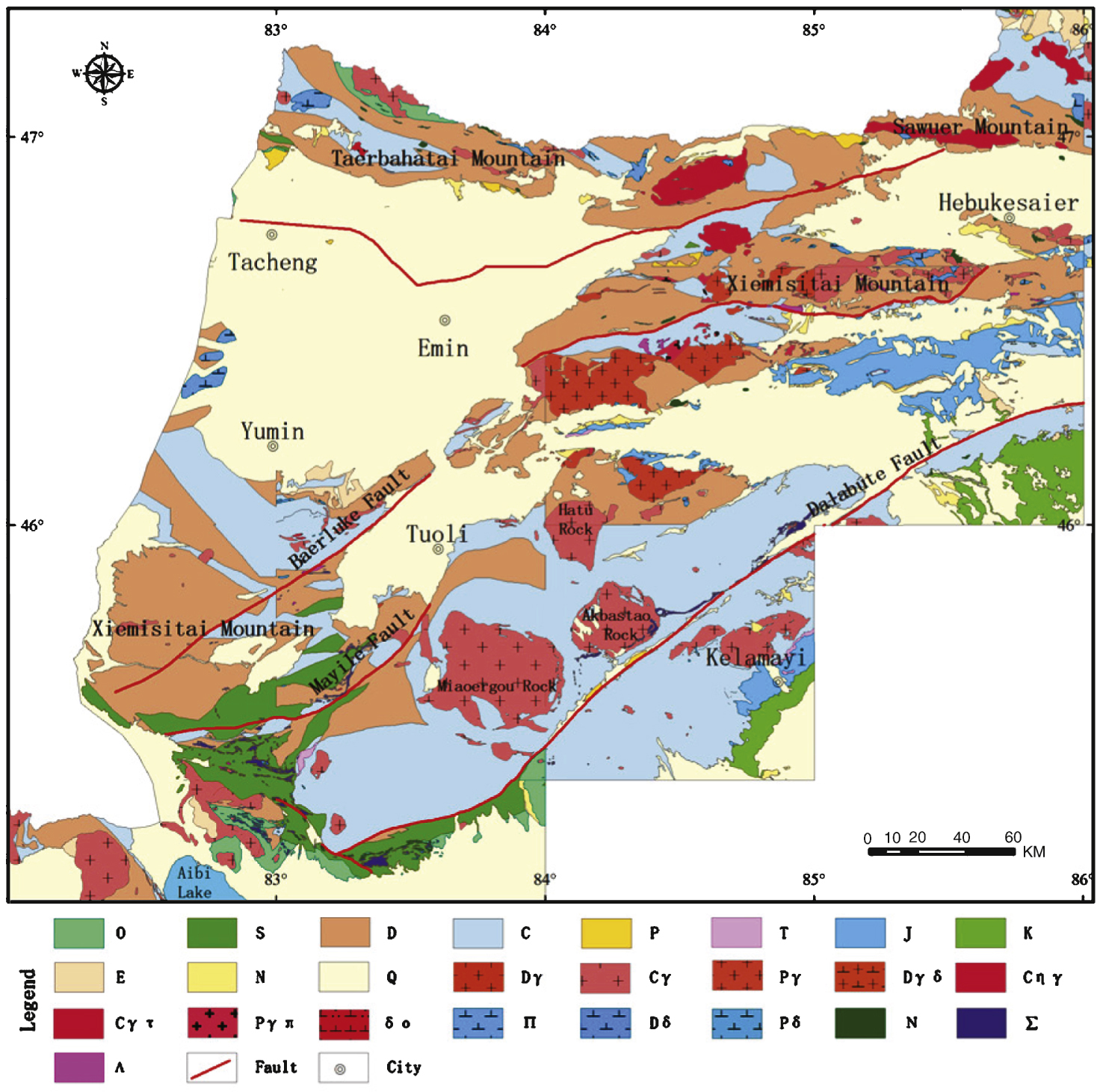
Fig.2
The effect of fuzzy gamma values (γ) on combining fuzzy memberships μ a and μ b to determine combined fuzzy membership μ c [18].
![The effect of fuzzy gamma values (γ) on combining fuzzy memberships μ
a
and μ
b
to determine combined fuzzy membership μ
c
[18].](https://content.iospress.com:443/media/ifs/2015/29-6/ifs-29-6-ifs1967/ifs-29-6-ifs1967-g002.jpg)
Fig.3
Spatial analysis map of nine layers.
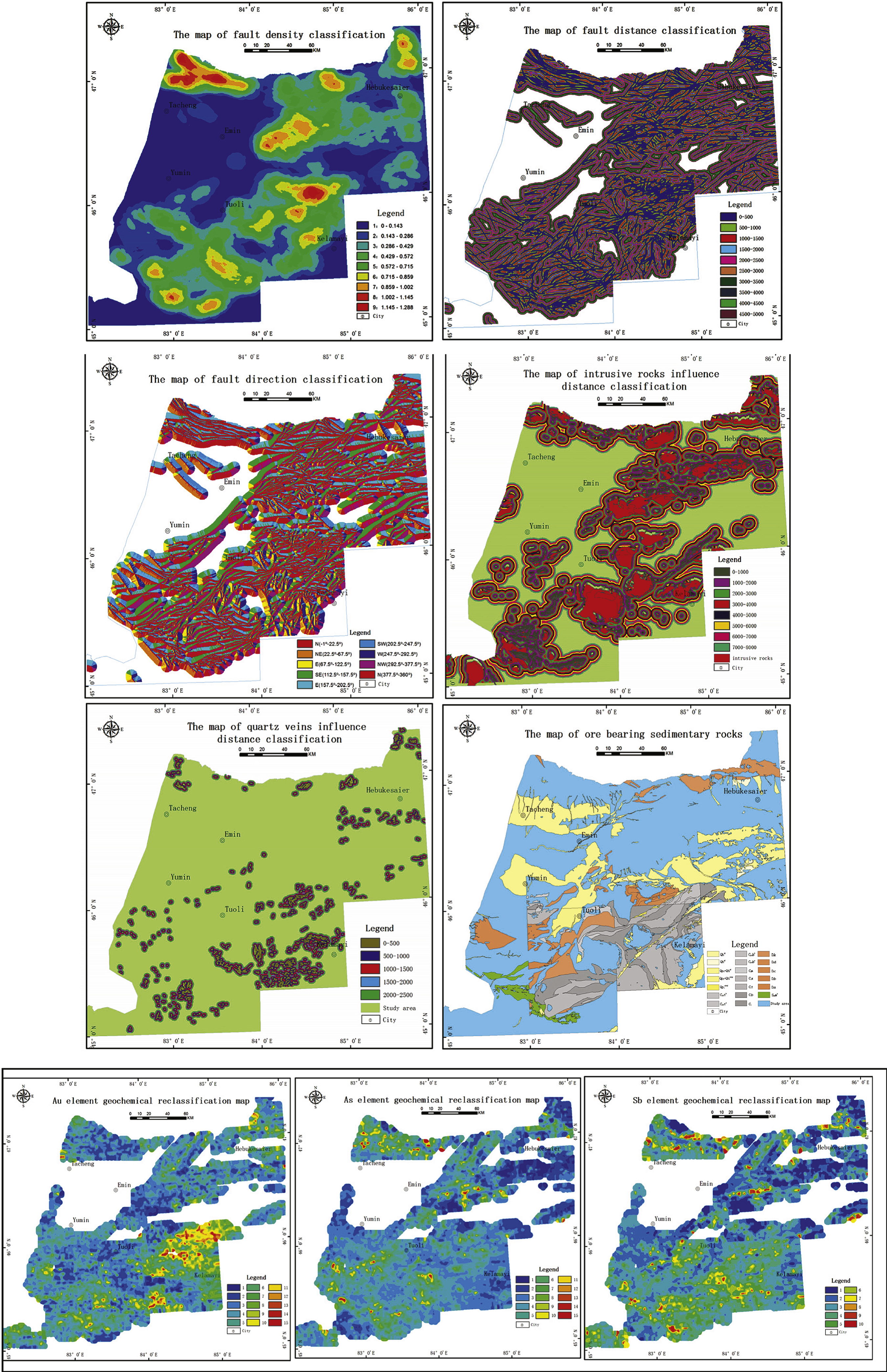
Fig.4
The cumulative relationship between posterior probability and study areas.
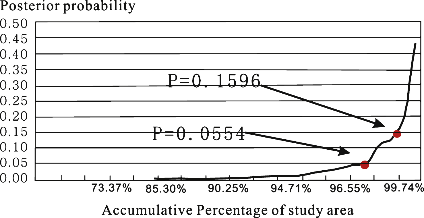
Fig.5
Mineral prospectivity mapping with W-of-E (having passed conditional independence test).
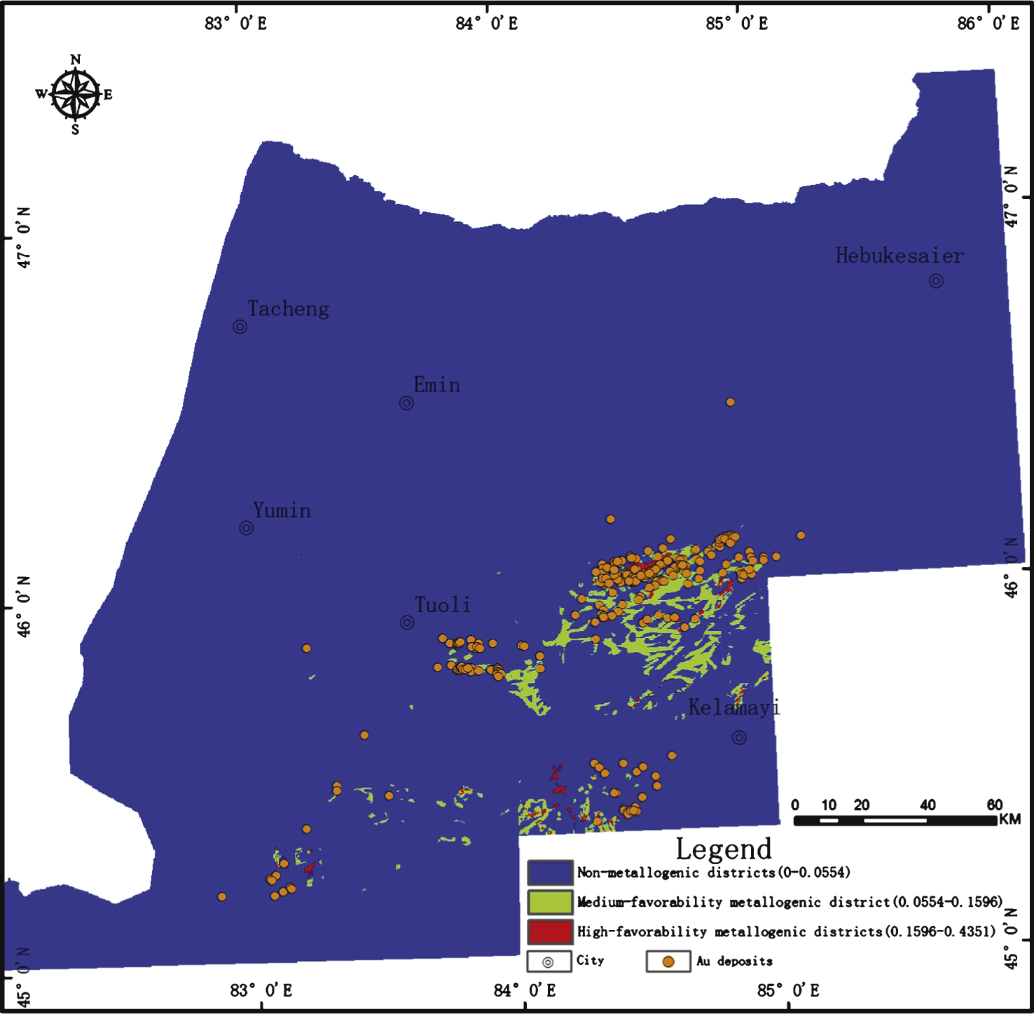
Fig.6
The inference network map of fuzzy logic.
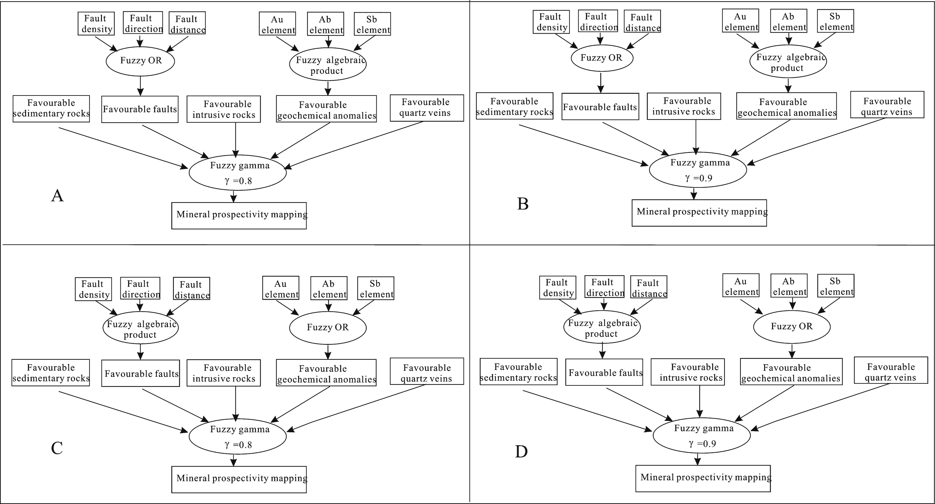
Fig.7
Mineral prospectivity mapping with fuzzy logic method.
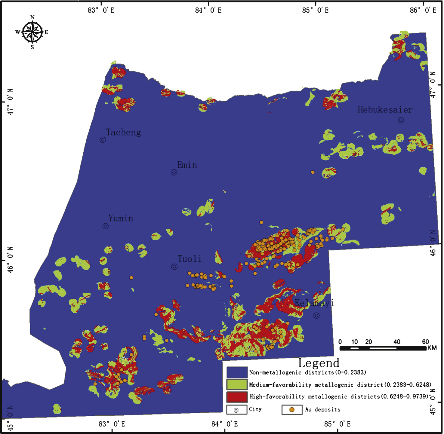
Table 1
The geological model of gold deposits in western Junggar
| Metallogenic factor | Contents of description | |
| Geological tectonic background | Tectonic environment | The NE-trending regional deep fault is the most important rock-controlling structure in this region. The position where the EW-trending deep fault converges with the NE-trending deep fault is usually the favorable metallogenic belt. |
| Intrusive rocks | The intrusion of intermediate-acid magma is closely associated with the formation of gold deposits. As the major metallogenic factor in this region, intermediate-acid intrusive rock has a special spatial relationship with ore deposits. | |
| Ore-bearing strata | Most of the gold deposits and gold occurrences in this region are concentrated in the middle-upper Carboniferous Tongbaogutu Formation and Tailegula Formation of the Paleozoic era. Lithologically, they are tuffaceous siltstone, siliceous tuff, and basalt. | |
| Wallrock alteration | Common forms of wallrock alteration include pyritization, arsenopyritization, carbonatization, siliconization and sericitization. | |
| Markers of gold-bearing dykes | Quartz veins are widely distributed in this region, especially in siliceous rocks. Gold deposits with industrial significance can be seen in some places. | |
| Regional geophysical field | Gravity | The gravity field in the gold deposit is elliptical, distribute in EW-NE direction. The contours near the faults are obviously twisted or linear. |
| Regional geochemical field | Au, As, and Sb elements are evenly distributed in each metallogenic sub-belt of the western Junggar area. Geochemical anomalies are common for Au, As, and Sb elements, with a narrow strip-like distribution pattern. As and Sb anomalies indicate anomalous mineralization. | |
Table 2
Quantitative evaluation of spatial relationship between gold deposits and nine evidential layers (S(C) > 1.0)
| Evidential Layers | Class | Area (km2) | Points | C | S(C) |
| Fault density | 0.572–0.715 | 4738.875 | 55 | 1.051 | 6.835 |
| Fault density | 0.715–0.859 | 3111.688 | 48 | 1.335 | 8.256 |
| Fault density | 0.859–1.002 | 1734.063 | 31 | 1.427 | 7.397 |
| Fault density | 1.002–1.145 | 500.438 | 23 | 2.365 | 10.730 |
| Fault density | 1.145–1.288 | 123.750 | 19 | 3.588 | 14.740 |
| Fault distance (m) | 0–500 | 13967.063 | 158 | 1.282 | 9.414 |
| Fault direction | –1°–22.5° | 5169.250 | 52 | 0.625 | 3.984 |
| Fault direction | 337.5°–360° | 7413.938 | 56 | 0.293 | 1.917 |
| intrusive rocks buffer (m) | 5000–6000 | 3178.875 | 21 | 0.234 | 1.003 |
| quartz veins buffer (m) | 0–500 | 1580.000 | 39 | 0.569 | 2.965 |
| Sedimentary rocks | D2 d | 96.813 | 43 | 4.792 | 26.984 |
| Sedimentary rocks | C2 - 3ba | 11.625 | 5 | 4.572 | 9.563 |
| Sedimentary rocks | C2 - 3bb | 80.125 | 17 | 3.860 | 14.929 |
| Sedimentary rocks | C2 - 3t | 55.688 | 11 | 3.757 | 11.867 |
| Sedimentary rocks | D2c | 88.938 | 13 | 3.451 | 11.873 |
| Sedimentary rocks | C2 - 3tb | 170.625 | 9 | 2.388 | 6.976 |
| Sedimentary rocks | C2m | 339.438 | 10 | 1.800 | 5.547 |
| Sedimentary rocks | C2x | 1665.938 | 37 | 1.617 | 8.986 |
| Sedimentary rocks | C1t | 1938.375 | 22 | 0.862 | 3.837 |
| Sedimentary rocks | C1b | 2704.125 | 30 | 0.860 | 4.386 |
| Au (ppb) | 1.8–2.1 | 1896.625 | 21 | 0.618 | 2.700 |
| Au (ppb) | 2.1–2.7 | 2298.688 | 22 | 0.465 | 2.077 |
| Au (ppb) | 2.7–3.3 | 1111.188 | 19 | 1.066 | 4.449 |
| Au (ppb) | 3.3–3.9 | 667.250 | 24 | 1.849 | 8.558 |
| Au (ppb) | 3.9–4.5 | 400.938 | 29 | 2.587 | 12.958 |
| Au (ppb) | 4.5–5.1 | 292.500 | 19 | 2.434 | 10.105 |
| Au (ppb) | 5.1–5.7 | 174.750 | 19 | 2.964 | 12.240 |
| Au (ppb) | 5.7–6.3 | 66.375 | 2 | 1.589 | 2.230 |
| Au (ppb) | 6.3–6.7 | 13.313 | 2 | 3.228 | 4.460 |
| As (ppm) | 12–16 | 10076.313 | 77 | 0.290 | 2.093 |
| As (ppm) | 16–20 | 5049.750 | 40 | 0.284 | 1.636 |
| As (ppm) | 20–24 | 2751.625 | 26 | 0.459 | 2.207 |
| As (ppm) | 24–28 | 1419.000 | 16 | 0.627 | 2.420 |
| Sb (ppm) | 0.6–0.8 | 11139.563 | 98 | 0.529 | 4.027 |
| Sb (ppm) | 0.8–1.0 | 7257.313 | 55 | 0.248 | 1.612 |
Table 3
The table of value of χ 2
| Evidential Layers | Sb content | Intrusive rocks | Fault distance | As content | Au content | Sedimentary rocks | Fault direction | Fault density |
| Quartz veins | 2.06 | 0.76 | 0.19 | 9.25 | 4.39 | 0.90 | 1.07 | 1.19 |
| Sb content | 0.09 | 0.01 | 2.79 | 5.72 | 0.04 | 0.07 | 2.43 | |
| Intrusive rocks | 0.92 | 8.72 | 7.48 | 0.19 | 4.10 | 7.31 | ||
| Fault distance | 0.02 | 1.93 | 0.09 | 19.48 | 18.69 | |||
| As content | 3.78 | 7.75 | 0.01 | 13.98 | ||||
| Au content | 0.18 | 0.98 | 35.62 | |||||
| Sedimentary rocks | 0.09 | 0.10 | ||||||
| Fault direction | 0.80 |
Table 4
Fuzzy membership value of faults
| Fault | Fault | Weight of | Weight of | Score of | Fuzzy membership |
| distance (m) | distance (m) | layer | class | class | value |
| 0–500 | 8 | 10 | 80 | 0.952574 | |
| 500–1000 | 8 | 6 | 48 | 0.450166 | |
| 1000–1500 | 8 | 5 | 40 | 0.268941 | |
| 1500–2000 | 8 | 3 | 24 | 0.069138 | |
| 2000–2500 | 8 | 4 | 32 | 0.141851 | |
| 2500–3000 | 8 | 6 | 48 | 0.450166 | |
| 3000–3500 | 8 | 2 | 16 | 0.032295 | |
| 3500–4000 | 8 | 6 | 48 | 0.450166 | |
| 4000–4500 | 8 | 1 | 8 | 0.014774 | |
| 4500–5000 | 8 | 6 | 48 | 0.450166 |
Table 5
Results of the four schemes
| Category | High-favorability | Number of |
| metallogenic districts | deposits covered | |
| A | 0.60% | 15 |
| B | 3.01% | 65 |
| C | 0.66% | 40 |
| D | 6.03% | 98 |
Table 6
Statistical results of fuzzy logic model
| High-favorability | Medium-favorability | Non-metallogenic | |
| metallogenic districts | metallogenic district | district | |
| Number of known deposits | 98 | 83 | 59 |
| Area covered | 6.03% | 8.06% | 85.91% |
| Highest posterior probability | 0.9739 | 0.6248 | 0.2383 |
Table 7
Comparison of weights-of-evidence model (having passed conditional independence test) and fuzzy logic model
| Number of deposits included | Highest probability of gold | Area of high-favorability | |
| in the high-favorability | mineralization | districts | |
| metallogenic districts | |||
| Weights-of-evidence model | 12 | 0.4351 | 0.17% |
| Fuzzy logic model | 98 | 0.9739 | 6.03% |

