Accuracy analysis of BLE beacon-based localization in smart buildings

Ivanov, Rosen

doi:10.3233/AIS-210607

Accuracy analysis of BLE beacon-based localization in smart buildings

Article type: Research Article

Affiliations: Department Computer Systems and Technologies, Technical University, Gabrovo, Bulgaria. E-mail: [email protected]

Correspondence: [*] Corresponding author. E-mail: [email protected].

Keywords: Indoor Positioning, BLE beacons, localization, smart sensor systems

DOI: 10.3233/AIS-210607

Journal: Journal of Ambient Intelligence and Smart Environments, vol. 13, no. 4, pp. 325-344, 2021

Published: 21 July 2021

Get PDF

Abstract

The majority of services that deliver personalized content in smart buildings require accurate localization of their clients. This article presents an analysis of the localization accuracy using Bluetooth Low Energy (BLE) beacons. The aim is to present an approach to create accurate Indoor Positioning Systems (IPS) using algorithms that can be implemented in real time on platforms with low computing power. Parameters on which the localization accuracy mostly depends are analyzed: localization algorithm, beacons’ density, deployment strategy, and noise in the BLE channels. An adaptive algorithm for pre-processing the signals from the beacons is proposed, which aims to reduce noise in beacon’s data and to capture visitor’s dynamics. The accuracy of five range-based localization algorithms in different use case scenarios is analyzed. Three of these algorithms are specially designed to be less sensitive to noise in radio channels and require little computing power. Experiments conducted in a simulated and real environment show that using proposed algorithms the localization accuracy less than 1 m can be obtained.

1.Introduction

The services people use in public smart buildings should deliver the information they want as quickly and reliably as possible. Such services aim to ensure a high level of visitor satisfaction. Satisfaction can be increased if the services are proactive. This means that services deliver personalized content to each client, predicting with high probability exactly what information they need at any given time. These services should take into account the profiles of their clients and should be adaptive to changes in the environment. For example, if a museum visitor approaches a painting, he/she will automatically receive information about the painting in preferred media formats. Such services are used when it is necessary to evacuate visitors from a building. In case of an emergency, each client of the service automatically receives information about the emergency, as well as a user-specific evacuation route. Services that depend on the position of their clients are called Location-Based Services (LBS). They are context-aware systems because the position is a type of context [28]. The concept of smart homes and smart public buildings is based on context-sensitive services such as LBS [30]. The usability of these services is directly related to the accuracy of determining the position of each client. Accurate calculation of this position would allow the creation of diverse and high-quality LBS. The use of Internet of Things (IoT)-based solutions [5,9] to calculate the position of visitors in buildings would increase the accuracy of these systems [30]. In this case, it will be possible to develop services that are adaptive to the changes in the building environment. At this stage, the cost of IoT-based building localization systems is too high. The reason for this is the need to build a sensor network in which each node should be able to exchange information with each of the other nodes. Based on this information, such a service could adapt to changes in the environment and thus minimize the error in calculating the position of its clients. At this stage, indoor positioning solutions use sensor networks with nodes, which operate independently [32]. Such solutions are less accurate and difficult to scale, but have a lower cost and do not require significant infrastructure changes. The accuracy of such services can be improved by using more accurate localization algorithms, as well as a more accurate estimate of the required sensor’s density (number of beacons per square meter) and placement [18]. The holistic approach to IPS design is the only way to ensure the development of IPS with optimal accuracy-price ratio.

Our general objective is to analyze the possibility of developing low-complexity IPS with an accuracy of less than 1 m using Bluetooth Low Energy (BLE) beacons as a sensor network [12,31]. The obtained results show that this is possible with an appropriate choice of algorithm for filtering the raw data from the beacons and for range-based BLE localization, taking into account the beacons’ density and placement shape.

The rest of the article is organized as follows. Section 2 is a critical review of the existing techniques and algorithms for indoor localization. Section 3 presents the algorithms analyzed in this article. In Section 4, the experimental results are presented. The paper is concluded in Section 5.

2.Related work

Many technologies can be used to create IPS [32]. The most common IPS uses a sensor network to calculate an estimate of the client’s (target) position. Sensor networks can use different types of sensor nodes, for example: infrared, visible light (Li-Fi), ultrasound, audible sound, and radio frequency (RF) [18,30,32]. These technologies have both advantages and disadvantages. For example, each technology requires changes in the infrastructure of the building. The aim is for these infrastructure changes to be small-scale and relatively inexpensive to implement. Some of these technologies (infrared, ultrasound, and Li-Fi) require additional hardware to be used by clients. At this stage, the most commonly used RF technologies for indoor localization are Wi-Fi, Ultra-Wideband (UWB), Radio Frequency Identification (RFID) and Bluetooth Low Energy (BLE) [30,32]. The main reason for this is the good ratio between localization accuracy and cost of development and implementation of such systems.

Localization systems using Wi-Fi and RFID have medium cost, complexity and accuracy. Wi-Fi-based indoor positioning systems require external power sources and additional pricey equipment. UWB-based systems have the highest localization accuracy (less than 0.5 m), but low security and the highest deployment cost due to the need for precise inter-node time synchronization. A battery-powered UWB dongle has to be attached to every client to measure his/her position. The client’s mobile device can read the calculated position over the Wi-Fi network.

One of the most promising technologies for locating visitors in buildings is BLE [12,31]. This technology guarantees low to medium localization accuracy at low system cost and medium to high security, depending on the version of Bluetooth standard. BLE is a Bluetooth SIG open-industry standard that aims to improve the performance of the Bluetooth Classic. The BLE devices operate in the 2.4 GHz ISM band at 2,400–2,483.5 MHz. It uses 40 RF channels, and each channel is 2 MHz wide. The improvements are related to better security, reduced maximum consumption, reduced latency, increased transfer rate, and increased maximum distance between BLE devices. Most BLE-based localization services use BLE beacons to implement their sensor networks. These devices are designed to generate push notifications for advertising purposes when a client of a service approaches an object (landmark). For this purpose, each BLE beacon sends the so-called advertising packets at a certain interval. The data packets are sent via three of the 40 radio channels. BLE technology works with: channel 37 (2,402 MHz), channel 38 (2,426 MHz), and channel 39 (2,480 MHz). Each packet contains information that is specific to each type of BLE beacon (iBeacon by Apple, Eddystone by Google, or manufacturer-specific BLE beacons). The data field in the iBeacon standard includes: iBeacon prefix, Universally Unique Identifier (UUID), Major, Minor, and TxPower.

BLE technology also has some drawbacks. BLE beacons can be used for the client’s localization, but distance estimate is quite inaccurate and varies depending on the environment and distance between BLE nodes. Mobile devices such as smartphones need from 2 to 4 seconds to detect a beacon in range. The open ISM frequency band used by BLE devices is filled with many other wireless protocols, such as Wi-Fi, as well as potential interference from home appliances. However, Wi-Fi has significantly higher output power, up to 23 dBm, compared to the maximum allowed 10 dBm for BLE standard. This means that placing a beacon very close to a Wi-Fi source will probably distort the transmitted data.

The main disadvantage of IPS using RF sensor networks is the dynamic variations in the parameters of radio channels due to the following more important factors: dimensions of rooms and corridors, type of construction material of the walls and ceilings, and position of static and dynamic objects in the building environment. In most RF-based localization systems, the calculation of the distance between the client and a sensor node is based on the value of Received Signal Strength (RSS) [26,34]. Regardless of the frequency, the value of the RSS attenuates approximately logarithmically with increasing distance between the reference node and the target node. Reducing variations in radio channel parameters is a difficult task that cannot be solved in real time when using mobile devices. The use of a mathematical model of the communication radio channel (free-space loss model, log-normal shadowing model, etc.) to predict the attenuation of RSS values does not give satisfactory results. The reason for this is that these models do not accurately describe the changes in the communication channel. The power of the transmitted signal from BLE beacons decays exponentially, mostly because of the distances, but there are also other effects such as fading and multipath effect that more or less affect the signal power. Fading is the time variation of the received signal. It depends on the environment and the movement of the objects. Multipath effect causes the signal to arrive in different ways to the device due to reflections, diffraction, and scattering. The most often used log-distance path loss model estimates RSS values measured at a location x from BLE beacon placed at a location x0:

(1)RSSk=RSS0k−10γklog10(ddo)+N(x0,x),

where RSSk value is an estimate for the signal power from kth beacon measured at distance d;RSS0k value is an estimate for the signal power from kth beacon measured at distance d0 (usually 1 m); γk is the path loss exponent, and N(x0,x) represents the random fluctuations in RSS due to different types of fading. The noise N(x0,x) is location-dependent shadow fading between the beacon and target node position. Usually, a log-normal distribution is assumed for noise:

(2)N(x0,x)∼N(0,σγ2),

where σγ2 is the shadowing variance. To localize the visitor, we should convert the RSS measurement (RSSI) to the estimated distance from the beacon:

(3)d=10RSSI0k−RSSIk−N(0,σγ2)10γk.

Path loss exponent γk may vary depending on the signal frequency and the building environment, from 1.5 m for Line-Of-Sign (LOS) scenario up to 3.5 for Non-Line-Of-Sign (NLOS) scenario. In a real environment, the radio channel between the target node and each reference node should be modeled. In practice, one model for the whole room or corridor is most often used. Experiments show that RSS signals in a dynamic environment have a multimodal rather than a unimodal distribution, and the communication channel is, most of the time, a nonlinear system. Therefore, nonlinear filters, such as Extended Kalman Filters or Particle Filters, should be used [13,16,20,33]. When these algorithms are implemented for multiple radio channels, they require too much computing power to be implemented in real time.

BLE-based localization algorithms can be split into two main categories [20]: distance-based and fingerprinting-based. Distance-based algorithms estimate target node position, calculating (directly or indirectly) the distance to three or more reference nodes. Distance-based algorithms [15] can be divided into two categories: 1) range-based algorithms and 2) range-free algorithms. Range-based algorithms [17] need to measure the distances between reference nodes and the target node. Then, the distances are used to calculate the position of the target node. Range-free algorithms [29] can indirectly obtain an estimate for the distances. Range-based algorithms have better localization accuracy compared to the range-free algorithms. Fingerprinting-based algorithms create a so-called reference fingerprint map using a vector of RSSI measurements in known positions [20]. Fingerprinting is an expensive localization technique that requires more deployment efforts and time. Any significant change in the infrastructure requires all measurements to be repeated in order to update the reference fingerprint map [8]. This technique is not suitable for use in large public buildings and dynamic environments. The fingerprint-based systems analyzed in [20] have an average localization accuracy of 2.5 m (from 0.8 m to 4.12 m). Similar accuracy is obtained with distance-based systems–2.1 m (from 0.75 m to 3 m). The reason for the differences between the minimum and maximum values of localization accuracy is the different parameters under which the experiments were conducted (room dimensions and deployment density). For example, in [7], the authors provide a BLE fingerprinting-based localization using 19 beacons distributed around 600 m². They achieved tracking accuracies of < 2.6 m 95% of the time using a dense beacon distribution (1 beacon per 30 m²) and < 4.8 m using a lower density distribution (1 beacon per 100 m²). In [10], the authors use fingerprinting localization in a hall of 7 m × 5 m, where the maximum distance between the target and reference nodes is less than 9 m. Using a trilateration algorithm, the average error is 2.8 m. Improving the accuracy of localization systems is possible by using various filtering techniques [16]. In [19], the authors use a Kalman Filter (KF) to reduce the localization error. The testbed consists of six BLE beacons located in the living room (8.5 m × 13 m) of a real house. The average localization accuracy was reduced to 1.77 m (41%) compared with the raw trilateration localization accuracy. In [33], the authors use the particle filtering method to improve localization accuracy. They report tracking errors low as 0.27 m in a smaller space and 0.97 m in a larger space.

3.Methods

3.1.RSSI data pre-processing

Fluctuations in RSSI data in buildings due to the presence of static (furniture, architectural objects) and dynamic (visitors) obstacles are the reason for the low localization accuracy. The radio frequency channels between BLE beacons and visitors are nonlinear systems. Accurate modeling of such systems is difficult to implement in real time using mobile devices. One possible compromise solution is to filter RSSI data so that for short intervals, the communication channel is a quasi-linear system. The most commonly used techniques for real-time filtering the observed set of RSSI values are the Moving Average (MA) filter and the Kalman Filter [10,16,27]. The KF is an optimal estimation method [20]. The KF algorithm can be described as a two-step process: the prediction step (time update) that makes use of the learned system dynamics to anticipate the next step of the system, and the correct step (measurement update) that takes a new observed measurement and uses it to correct the system dynamics and state. For IPS, the level of measurement noise is environmental and visitor movement dependent. In this case, the KF is not optimal and may cause unreliable results. One solution for solving the problem is to use adaptive Kalman filtering.

This article proposes the combination of MA filter and an Adaptive Kalman Filter (AKF) as a novel dynamic noise reduction algorithm. The algorithm uses signal processing at the time window level. For each time window (N number of RSSI values) the average (uavg), maximum (umax), and minimum (umin) RSSI values are calculated. A MA filter is used to obtain the average value of input signal u:

(4)uavg=1N∑i=1Nui,

The following parameter Δu is used to estimate RSSI fluctuations within the time window:

(5)Δu=umax−umin.

The proposed AKF algorithm is used to filter uavg, umax and umin values. In this case, the AKF is one dimensional. If RSSI data are analyzed in one-second intervals, the time transition matrixes are one second. In this case, process noise was the same as the measurement noise. Thus, AKF equations are reduced to the following form:

(6a)xˆk−=xˆk−1Pk−=Pk−1+qKk=Pk−/(Pk−+r)(6b)xˆk=xk−+Kk(zk−xk−)Pk=(1−Kk)Pk−

where k is discrete time, xˆk− is a priori state estimate, xˆk is a posteriori state estimate, Pk− is a priori estimate for error covariance, Pk is a posteriori estimate error covariance, Kk is the Kalman gain matrix, and zk is the observed data (RSSI). It is assumed that the process noise variance q is constant (q=0.2). A filtered signal xˆk is calculated based on an estimation of the difference between measured value zk and a priori state estimate xˆk−. To obtain the degree of filtering of RSSI data, it is proposed to use fuzzy logic to estimate the value of measurement noise variance r (6a). Two input fuzzy variables are used (see Fig. 1). First input variable DeltaRSSI estimates error in the RSSI data. We use parameter Δu obtained with (5) as value for this input variable. Four values for DeltaRSSI are used: S (Small), MS (Medium Small), MH (Medium High) and H (High). It is assumed that the lower the DeltaRSSI value, the less RSSI data should be filtered. When visitors move into the building, the use of non-adaptive Kalman filters often results in over-filtering. In this case, the filter convergence time may reach several seconds.

Fig. 1.

Fuzzy membership functions.

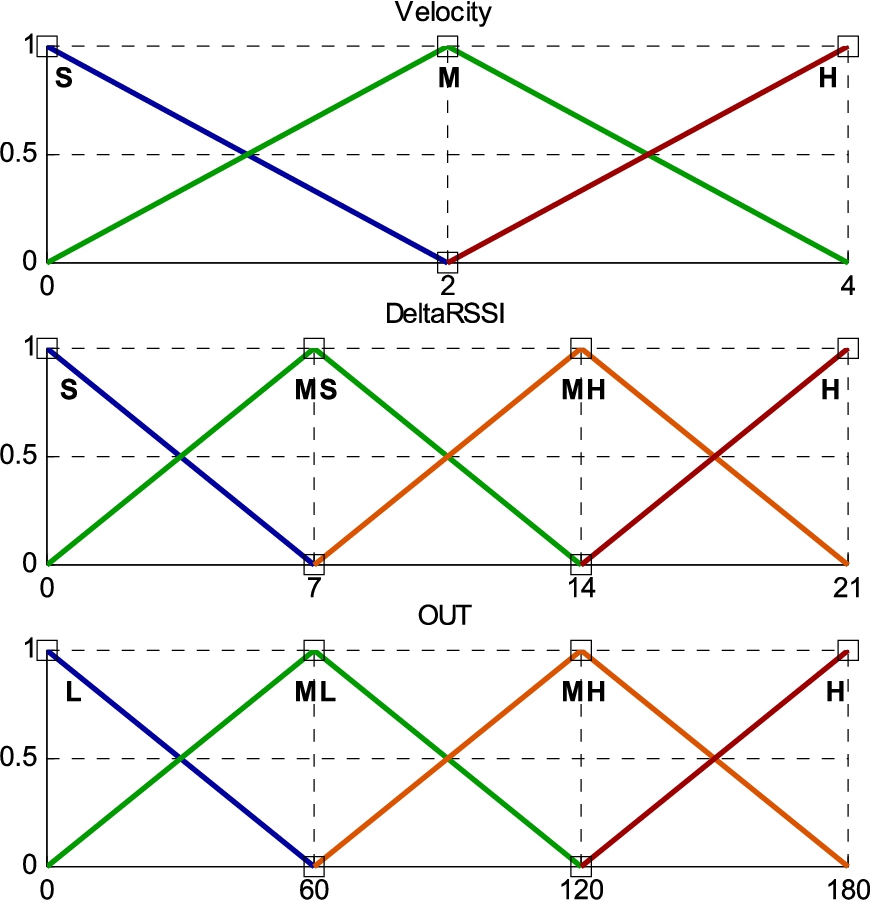
To prevent this, the visitor’s speed of movement is used as second input variable (Velocity). The values of the variable Velocity are following: S (Small), M (Medium) and H (High). The faster the visitor moves, the less RSSI data is filtered. The possible values for output linguistic variable OUT are following: L (Low), ML (Medium Low), MH (Medium High) and H (High). The higher the OUT value, the stronger the input data is filtered. To obtain output linguistic variable OUT, 12 fuzzy rules of the following type are used:

if Velocity=value AND DeltaRSSI=valuethen OUT=value.

Figure 2 shows the fuzzy rule matrix used. To infere logical products for each rule, Root-Sum-Square method is used. The defuzzification of the data into a crisp output is realized by combining the results of the inference process and the computing of the fuzzy centroid of the area.

Fig. 2.

Fuzzy rule matrix.

3.2.Localization algorithms

This article analyzes the accuracy of five range-based localization algorithms in different use case scenarios. The first two well-known algorithms–Trilateration and Nonlinear Least Squares (NLLSQ) localization–are used for comparison with the other three algorithms, which are specially designed to be less sensitive to noise in radio channels and require little computing power.

Trilateration is one of the most commonly used range-based techniques for localization in buildings [1,3,6,22,27]. Three RF sources, such as BLE beacons, placed in known locations, are required to calculate the 2D position of the target node. When using three beacons, the position of the client is the point at which all circumferences intersect. In real indoor environments, due to the fluctuation of the RSSI values, instead of intersecting at one point, these three circles can either intersect in an area, or not. Therefore, we use Line Intersection-based Trilateration algorithm [21] to estimate visitor’s position.

Nonlinear Least Squares [27] is an optimization technique that solves nonlinear data-fitting problems of the following 2D form:

(7)minx,y‖f(x,y)‖22=minx,y(f1(x,y)2,+⋯+fn(x,y)2).

When the position needs to be calculated, the function to be minimized is as follows:

(8)f=(x−xi)2+(y−yi)2−di2.

where (x,y) is the estimated position of target node, (xi,yi) is the position of ith beacon, and di is the distance between ith beacon and estimated target node position, which is calculated using (3). This algorithm starts at the point p(x0,y0) and returns estimated target node position when function f goes under the predefined threshold. The position of the starting point is calculated using Weighted Centroid Localization algorithm [24]. In order to be able to estimate the position of target point, two or more distance estimates should be available for the distances between the visitor and two beacons (the number of observations should be equal or greater than the number of unknown parameters).

3.3.First proposed algorithm (ALG-1)

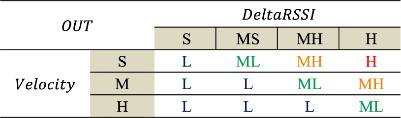
The proposed algorithm ALG-1 belongs to the range-based localization algorithms but implements some ideas used in the range-free localization algorithm named Ring-Overlapping Circle RSSI (ROCRSSI) [15]. The ROCRSSI algorithm requires beacons to be able not only to transmit data, but also to read the data from other beacons. This makes it unusable if standard BLE beacons are to be used. Let us assume that RSSIi is the signal from ith beacon and RSSIt is the signal from the target node. If RSSIi<RSSIt then the ith beacon belongs to Group 1. Otherwise, it belongs to Group 2. The maximum RSSI value in Group 1 is used to calculate radius r1 and the minimum RSSI value in Group 2 gives radius r2. It is assumed that target node is located between two circles (ring) with inner radius r1, outer radius r2 and center coincided with a beacon’s position. Repeated for all the beacons, a set of overlapping ring pairs are created. The target node is located as the center of gravity of these overlapping ring pairs.

In our case we use standard BLE beacons. The aim is to obtain an estimate for the values of radii r1 and r2 without it being possible for each beacon to receive the RSSI value from the other beacons. For this purpose, RSSI fluctuations from each beacon are analyzed and filtered using proposed AKF. The attenuation of the RSSI signal is more significant when there are objects or people between the visitor and these nodes. In this scenario, the target node will receive a lower value for the power from the BLE node. The attenuation of the power can be modeled by assuming that the position of the target node is within a ring whose outer radius is proportional to this attenuation. From the coordinates of the overlapping parts of the rings obtained for two or more beacons, an estimate of the target node position can be obtained. We use weighted centroid to calculate the final estimate for the position. To obtain the inner and outer radii of each ring, the maximum and minimum RSSI values for each time window are filtered using combination of the MA filter and AKF described in Section 3.1. Based on these values (uˆmax, uˆmin), the inner and outer radii of the ring are calculated. The values of r1 and r2 are obtained using the path loss model (1):

(9)r1=10RSSI0−uˆmax10γ,r2=10RSSI0−uˆmin10γ.

The calculation of the estimated target node position is realized in the following sequence (see Fig. 3a). First, we select beacons involved in obtaining the target node position. For each beacon the radii r1 and r2 are calculated using (9). Second, the coordinates of all intersections between rings are obtained.

Fig. 3.

Localization using algorithm ALG-1: (a) how algorithm works: valid intersections (blue dots); invalid intersections (red dots); estimated position of target node pt (red diamond); (b) algorithm in action: ΔRSSI = ± 6 dBm; target point (blue circle); circle with r=1 m (dark yellow).

If the number of intersections between each possible pair of circles is two, the one for which a less total distance from the point to the position of the selected beacons is winner point (blue dots). The other point is considered invalid and is removed (red dots). Finally, it is assumed that the position of the target node pt (red diamond) coincides with the coordinates of the weighted centroid of area that blue points form. Higher weights are set for intersections that have a smaller total distance to the selected nearest beacons:

(10)wi=1/∑∀k‖piint,pkbeacon‖,

where piint is the position of an intersection point with an index i; pkbeacon is the position of a beacon with an index k; ‖·‖ is the distance between two points in a Cartesian coordinate system.

The estimation for position of the target node pt is obtained using the following equation:

(11)pt=∑∀i(wipiint)/∑∀iwi.

Figure 3b shows how the ALG-1 works when three beacons are selected to estimate position of target node. Random noise in RSSI data with a maximum value of ±6 dBm is added. The blue circle is the real position of the target node, and the red diamond–the estimated position. The accuracy of the algorithm is highest if the target node position coincides with the center of gravity of an area that the beacons form (triangle B₂B₄B₅).

3.4.Second proposed algorithm (ALG-2)

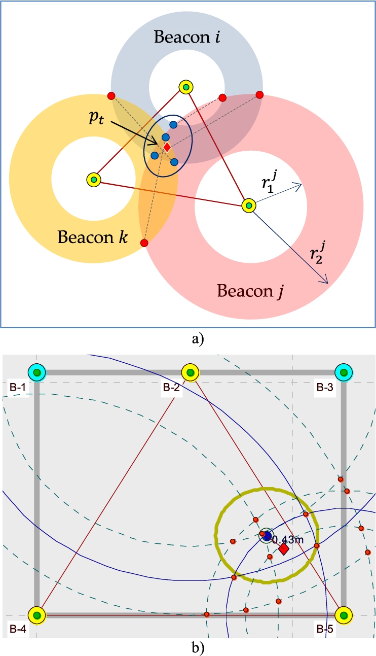
The main reason for the error in estimating the target node position in the Trilateration and NLLSQ algorithms is the inaccurate calculation of the distance between the target node position and the beacons. In algorithm ALG-2, the target node position is calculated based on the difference between the RSSI values for each pair of beacons involved in the position-finding process. Therefore, each RSSI difference value is proportional to the ratio of the distances between the target node and each pair of beacons. If all beacons are configured to transmit at the same power, then this parameter (TxPower) will not affect the accuracy of position calculation. In the proposed algorithm, in order to simplify the calculations, it is assumed that the position of the target node is located in the center of a polygon. Let us first consider a special case in which the position of the target node is a point pij with coordinates (x,y), which lies on a line connecting two beacons with indices i and j (see Fig. 4a). In this case, the target node position pij is obtained by the following equations:

(12)x=xi+didi+dj(xj−xi)=xi+xj−xi1+cof,y=yi+didi+dj(yj−yi)=yi+yj−yi1+cof.

where cof=dj/di, dk is the distance between the target node position and a beacon with index k. The value of parameter cof can be obtained using (3). If all beacons transmit with equal power, the value of this coefficient is obtained by the following equation:

(13)cof=10RSSIi−RSSIj10γ=10RSSDij10γ.

Fig. 4.

Localization using algorithm ALG-2: (a) how algorithm works: target point (blue circle); intersection points (red circles); (b) algorithms ALG-2A and ALG-2B in action: ΔRSSI = ±3 dBm; circle with r=1 m (dark yellow); estimated position of target node using ALG-2A algorithm (green triangle up); and estimated position of target node using ALG-2B algorithm (green triangle down).

Let us consider a case in which the position of the target node is a point pt, which falls into the triangle formed by three beacons with indices i, j, and k (see Fig. 4a). Let us assume that the projections of this point on the lines between each pair of beacons are the points pij, pik, and pkj. If there is no noise in the RSSI data, then the target position is obtained as an intersection between the lines l⊥ij, l⊥ik, and l⊥kj. The line l⊥ij is perpendicular to the line lij, which connects beacons i and j and passes through the point pij. For the equation of line l⊥ij, we can write:

(14)y=ypij+m⊥ij(x−xpij).

In order for a line l⊥ij to be perpendicular to a line lij, the following condition should be satisfied:

(15)m⊥ij=−1mij=−xj−xpijyj−ypij,

where mij is the slope of the line lij. The equations for the other perpendicular lines l⊥ik and l⊥kj are found in a similar way. It remains to find the intersections between each pair of lines (l⊥ij, l⊥ik), (l⊥ij,l⊥kj) and (l⊥ik,l⊥kj). The condition l⊥ij∩l⊥ik≠∅ is satisfied if l⊥ij=l⊥ik. In this case, for the coordinates of the intersection point pinti between the lines l⊥ij and l⊥ik, the following equations are obtained:

(16)xinti=ypik−ypij+m⊥ijxpij−m⊥ikxpikm⊥ij−m⊥ik,yinti=ypij+m⊥ij(x−xpij)

The coordinates of the other intersection points are obtained in a similar way. The estimated target node position coincides with the center of gravity of the area obtained from all three intersections:

(17)pt=pinti+pintj+pintk3.

If n is the number of beacons used to calculate the position of the target point, the algorithm can be used if n⩾2. Two variants of the proposed algorithm will be analyzed. In the first variant (ALG-2A), the position of the target node coincides with the position of the point calculated using (17). In the second variant of the algorithm (ALG-2B), the target node position coincides with the position of one of the intersection, for which a minimum sum of distances between the intersection point and the points on the sides of the triangle involved in calculating its coordinates:

(18)pt=min∀m(∑∀q∖m‖pintm,pmq‖).

The accuracy of these algorithms depends on the geometric location of the beacons involved in the position calculation (see Fig. 4b). Best localization accuracy is obtained if the target node is in the center of a triangle that beacons form. When the target node is located in the triangle that the beacons form, the accuracy of algorithms ALG-2A and ALG-2B is approximately the same. Worst localization accuracy is obtained when the position of the target point is outside of the triangle. In this case, as shown in Fig. 4b, the ALG-2B algorithm has better accuracy than the ALG-2A algorithm.

4.Experiments

In this section, several use case scenarios are conducted to analyse localization accuracy of the algorithms described in Section 3. The analysis of the parameters on which the localization accuracy depends is realized through a testbed platform, which includes: 1) Mobile app which dump to CSV file information from beacons with highest RSSI values and data from built-in accelerometer; 2) Texas Instruments (TI) CC2540 USB BLE dongle and SmartRF BLE packet sniffer software; 3) Java app for raw BLE packets data pre-processing and dump; and 4) Matlab™ software for automatic beacons deployment and localization algorithms comparison.

Mobile apps for BLE beacon configuration are most often specific to each manufacturer (Gimbal, Kontakt.io, iBKS, etc.) in order to ensure a higher level of security. Through them, the beacons can be configured by setting a specific value for each parameter, for example, advertising interval, Major, Minor, RSSI0, and TxPower. Using TI CC2540 BLE dongle, it is possible to scan any BLE channel for data from BLE devices. Data from CC2540 is analyzed using TI SmartRF BLE packet sniffer software. It allows setting the identifier of the BLE channel, which should be sniffed, as well as how to visualize the contents of the data packets. The application allows broadcasting BLE packets to other applications using UDP protocol. A Java application that starts a UDP server to capture packets transmitted by the SmartRF packet sniffer is developed. This app allows real-time recording of raw and filtered data as CSV files. Subsequently, this data is processed by a Matlab™ application that allows statistical analysis of data from CSV files.

4.1.Use case scenario 1

The aim of the first experiment is to analyze the applicability of the algorithm for beacon’s data pre-processing. The experiment was conducted in a lecture hall for 50 students. The dimensions of the hall are 11 m × 6 m × 3.3 m. Six BLE beacons were used, four of which were located in the corners of the hall, and two were located in the middle of the longer sides of the hall. They are located at a height of 1.5 m from the floor of the room. The same configuration parameters are set for all beacons: advertising interval (200 ms), RSSI0 (−52 dBm), and TxPower (4 dBm). To obtain the parameters of the log-distance path loss model, Matlab™ cftool is used (see Fig. 5).

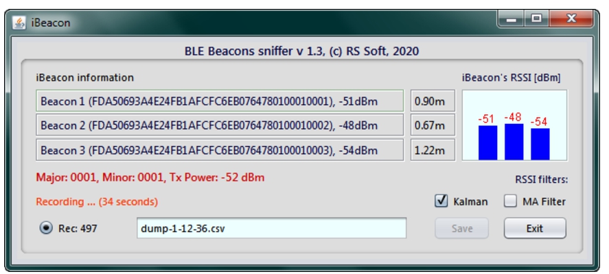
The SmartRF BLE packet sniffer software is used to select a specific BLE channel (37, 38 or 39) to read beacon’s packets. The developed Java app starts a UDP server and capture packets transmitted by the TI SmartRF packet sniffer. This application has a graphical user interface (see Fig. 6) and allows: 1) Initialization of the app using parameters from a configuration file (minimum value of RSSI below which the data from the corresponding beacons is not processed; UUID of the beacons to be analyzed; maximum number of beacons to be analyzed; filter parameters, etc.; 2) Real-time visualization of RSSI data from the three closest to target node beacons; 3) Filter type selection: MA filter, Kalman filter or a combination of both filters; 4) Start / stop saving data into a CSV file – the application shows how many samples are recorded and how much time has elapsed since the beginning of the recording.

Fig. 5.

Lecture hall path loss model, γ=2.533 (95% confidence bounds).

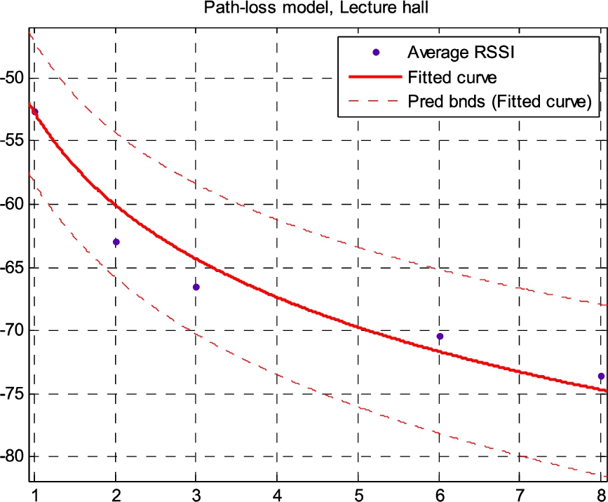
Fig. 6.

Java app for beacons data pre-processing and dump.

One hundred records received from different beacons and channels were analyzed for the specific distance between target and reference nodes, and noise in the BLE chanels. For each of the five distances (1 m, 2 m, 3 m, 6 m, and 8 m), 20 records were obtained. Each record contains about 500 samples (100 seconds). Matlab™ software is used to visualize the results obtained. The length of the time window N is set to 10 samples. AKF returns a result every second. To make this possible, a 50% overlap of time windows is used. In order to analyze the proposed AFK, two types of experiments have been implemented in a real environment. During all tests, there is a movement of people crossing the line that is formed when connecting the positions of the reference (beacon) and target node (visitor). The aim is to simulate the alternation of LOS and NLOS scenario. In the first experiment, the RSSI data obtained from a target node that is stationary and located at a specific distance (dref) from the reference node are analyzed. Figure 7 shows the results obtained after analyzing two records at a distance between nodes of 1 m and 8 m. Large decreases in RSSI values occur when the direct visibility between the two nodes is lost. An overall summary of the results for all distances are shown in Table 1. For each filtering algorithm and for each reference distance between the beacons, the min, max and average distances were calculated, as well as the standard deviation. It can be clearly seen that in a dynamic building environment, fluctuations in RSSI data result in large errors in the calculated distance between the nodes – from 0.24–1.72 m at dref=1 m to 3.3–7.3 m at dref=8 m.

Fig. 7.

Beacon’s data pre-processing – raw data (green), filtered data (MA + AKF): average curve (green circles), maximum curve (red), and minimum curve (blue): (a) 1 m distance between reference and target nodes; (b) 8 m distance between nodes.

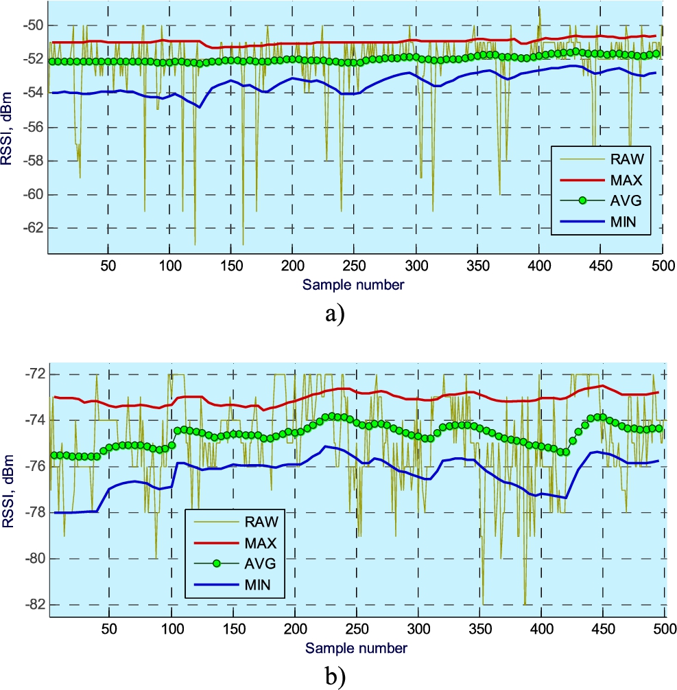
Table 1

Summary of result obtained in dynamic environment with the static target node used

Filtering algorithm		Distance, m

Error, m		1	2	3	6	8
Raw	min	0.24	0.91	1.34	2.05	3.31
	max	1.72	4.16	8.22	8.10	7.29
	avg	0.04	0.13	0.23	0.28	0.35
	std	0.24	0.39	0.77	0.98	1.41
MA	min	0.10	0.22	0.70	0.89	1.84
	max	0.33	0.44	0.85	1.42	2.39
	avg	0.03	0.11	0.28	0.24	0.18
	std	0.08	0.12	0.38	0.47	0.95
MA + AKF	min	0.02	0.01	0.12	0.46	0.73
	max	0.04	0.20	0.54	0.78	1.53
	avg	0.003	0.10	0.18	0.23	0.25
	std	0.016	0.05	0.15	0.28	0.72

Fig. 8.

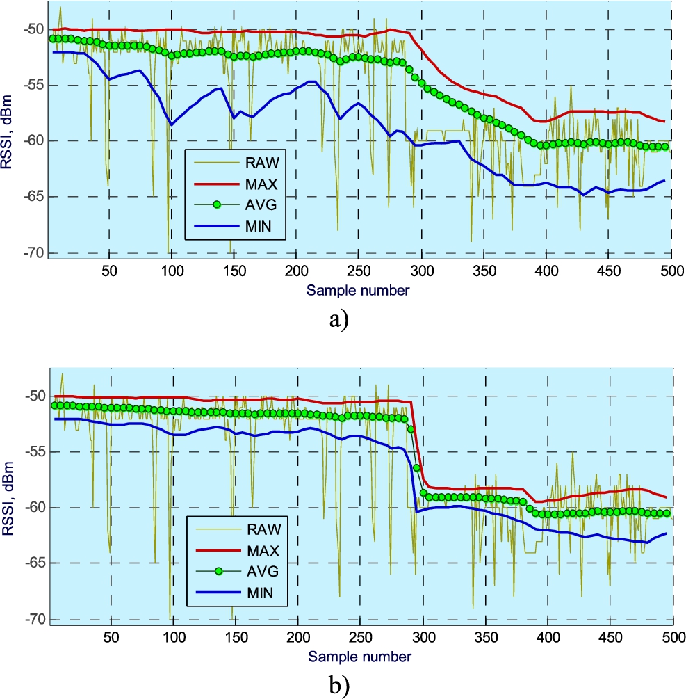
Beacon’s data pre-processing in dynamic environment and moving target node: (a) non-adaptive KF is used; (b) proposed AKF is used.

When using an MA filter, the error in the calculated distance decreases, but for dref>3 m it is over 1 m (0.9–1.42 m for dref=6 m and 1.84–2.39 m for dref=8 m). When using a combination of MA filter and proposed AFK (Velocity=0), the maximum error for all tested reference distances is less than 1 m.

In the second experiment, the target node (visitor) moves in the lecture hall from one reference distance between the nodes to another reference distance. The visitor uses a mobile app through which the data from the six beacons and his/her speed of movement are recorded in a CSV file. Using Matlab^™, it is analyzed for how long the reaction of a non-adaptive KF and the proposed AKF converge to the actual value of RSSI. During all the recordings, people move in the room. Figure 8 shows the result after filtering the RSSI data obtained by moving the target node from the reference node at an initial distance of 1 m (−52 dBm) to a final distance of 2 m (−60 dBm). It is clear that when using a non-adaptive Kalman filter (Fig. 8a) the convergence time is over 100 samles (20 seconds). When using the proposed AFK (Fig. 8b), this time is reduced to 15 samples (3 seconds). Experiments show that a non-adaptive Kalman filter does not give satisfactory results if the target node is not stationary. In this case, the convergence of the KF is insufficient to take into account the dynamics of the target node.

Fig. 9.

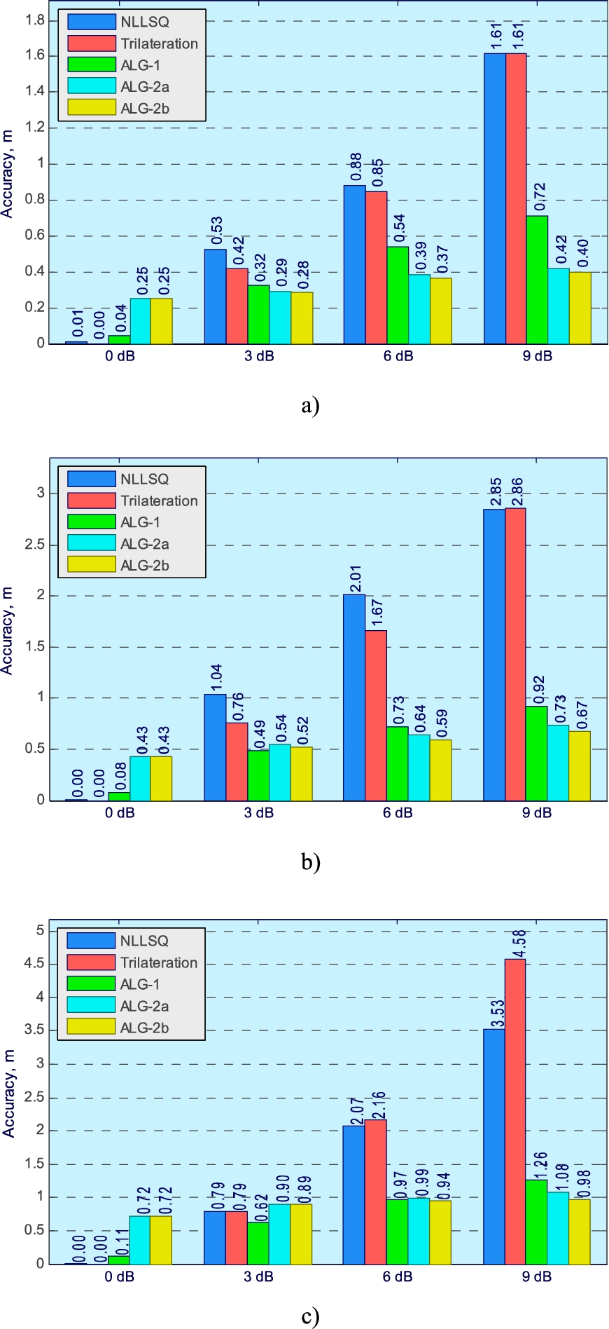
Comparison of algorithms localization accuracy: (a) distance between beacons is 3 m; (b) distance between beacons is 6 m; (c) distance between beacons is 9 m.

4.2.Use case scenario 2

The aim of the second experiment was to validate the localization algorithms in an simulated environment at different target node positions relative to the reference nodes position, different values of the fluctuationsin the RSSI values, and different distances between the reference nodes (beacons). To validate the algorithms, localization accuracy is calculated. The localization accuracy εt is the measure of the correctness of the obtained estimate for the position of the target node, which is calculated as the difference between the actual position of the target node, pt=(xt,yt) and the estimate for this position, pˆt=(xˆt,yˆt):

(19)εt=(xt−xˆt)2+(yt−yˆt)2.

All experiments were performed under the assumption that the signals from three reference nodes were analyzed, which form an equilateral triangle. The accuracy of localization at three different distances between the beacons (3 m, 6 m, and 9 m) and three different positions of the target node is analyzed. We test localization accuracy for the following target node positions: 1) Target node is in the center of an equilateral triangle; 2) The position of the target node coincides with the position of an reference node; and 3) The target node is outside the triangle. For each of these three positions, 50 estimates were made for the target node position at four different maximum values for the random noise level in RSSI (0 dBm, ±3 dBm, ±6 dBm, and ±9 dBm). Figure 9 shows the average localization accuracy estimates for all possible target node positions at different distances between reference nodes and noise in RSSI values. The ALG-2A and ALG-2B algorithms have almost constant accuracy for all values of noise and distances between reference nodes. This is expected because ALG-2 algorithms are not significantly affected by noise in RSSI data. The more accurate is ALG-2B, which guarantees average localization accuracy less than 1 m for all test scenarios. The ALG-1 algorithm has approximately the same accuracy as the ALG-2 algorithms for noise in RSSI data up to ±6 dBm. Trilateration and NLLSQ algorithms can be used for micro-localization only at a small distance between beacons and low noise levels in communication channels. These requirements cannot be guaranteed in a real environment. Analysis of the position of the target node shows that all algorithms are most accurate when the target node is at the center of gravity of the triangle the three nearest beacons form. However, at this target node position, the Trilateration and NLLSQ algorithms guarantee micro-localization only when the distance between the beacons is less than 3 m. The ALG-1 and ALG-2 algorithms are most inaccurate when the position of the target node is outside the triangle the reference nodes form. In this case, these algorithms guarantee micro-localization only if the distance between reference nodes is less than 6 m.

4.3.Use case scenario 3

This experiment analyzes how the beacons’ density and deployment shape affect the accuracy of the localization algorithms [4,11,24,25,27]. The localization accuracy increases as the distance between the beacons decreases. In large public buildings, the cost of the deployment increases as the distance between the beacons decreases. For this reason, a compromise should be made between the deployment cost and the localization accuracy. Experiments show that in addition to the beacons’ density, the localization accuracy also depends on the shape the beacons form. In [24], the authors prove that the best placement of beacons is when every three of them form an equilateral triangle. This shape is called Crystal-shape iBeacon Placement (CiP), and it gives better results compared to the Z-curve placement strategy described in [23]. In a real building environment, these shapes cannot be guaranteed due to the specific dimensions of the rooms and corridors as well as the need for different localization accuracy in different rooms and corridors.

Matlab™ software has been developed to deploy beacons automatically, taking into account the desired shape and deployment density. All analyzed localization algorithms were tested for a simulated space of 200 m² (20 m × 10 m) in the following two scenarios:

CiP shape and a distance between the beacons 5 m (5 beacons) and 10 m (14 beacons).
Rectangular shape and a distance between the beacons 5 m (6 beacons) and 10 m (15 beacons).

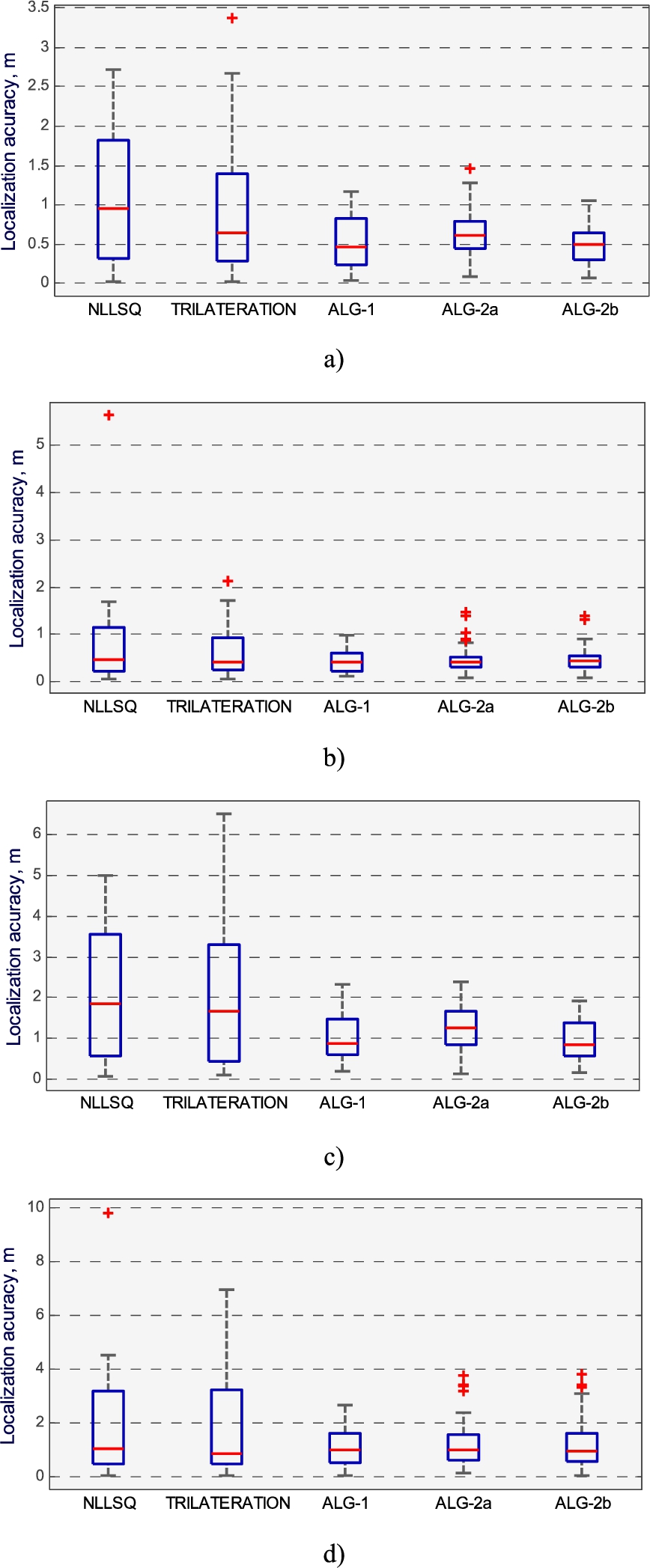
For each scenario, the localization accuracy was analyzed for 50 test points with pseudo-random coordinates. Different random noise with maximum amplitude of ±5 dBm has been added to the RSSI data. The obtained results are shown in Fig. 10 as a box-and-whisper plot. Trilateration and NLLSQ algorithms have better localization accuracy if a CiP shape is used. Conversely, ALG-2 algorithms have better accuracy if a rectangular shape is used. The reason for this is that ALG-2 algorithms have less accuracy when the target node is outside the triangle formed by the nearest beacons. Such a scenario is possible due to the noise in the radio channels. The localization accuracy of the ALG-1 algorithm depends less on the deployment shape and beacon’s density compared to other algorithms. At a distance between the beacons of 5 m, only the ALG-1 and ALG-2B algorithms can be used for micro-localization. For example, for a CiP shape, the accuracy of the ALG-1 algorithm is less than 1 m for all test points. In this case, the ALG-2A algorithm has three test points, and the ALG-2B algorithm has two test points for which the localization accuracy is over 1 m but less than 1.5 m. At a distance between the beacons of 10 m, the best localization accuracy has the algorithm ALG-2B when a rectangular shape is used. In this case, none of the localization algorithms guarantees accuracy below 1 m for all test points.

Fig. 10.

Comparison of different type of beacon deployment–box-and-whisper plot (n=50, ΔRSSI = ±5 dBm): (a) rectangle shape, d=5 m; (b) triangle shape, d=5 m; (c) rectangle shape, d=10 m; (d) triangle shape, d=10 m.

4.4.Use case scenario 4

The aim of this use case scenario is to validate the analyzed beacon’s data pre-processing and localization algorithms in a real indoor environment. Specially developed apps for Android OS and Matlab™ are used to realize this scenario. The experiment was conducted in a lecture hall described in Section 4.1.

Two experiments were performed in this scenario. The first experiment analyzes the accuracy of the localization algorithms at nine test points in the room (see Fig. 11). The positions of these points are selected to simulate different positions of the test point relative to the positions of the beacons. When a participant in the experiment reaches a test point, he/she presses a button so the mobile app can receive information about this event. The route with test points is passed 20 times in one day.

During the experiment, five people move into the room. The software saves in a CSV file the information from beacons and accelerometer every 200 ms. The Matlab™ software calculates the localization accuracy for each analyzed algorithm at all test points (see Fig. 12).

Fig. 11.

Test environment–lecture hall: beacons (red rectangles); test points (gray circles); furniture (yellow and green rectangles).

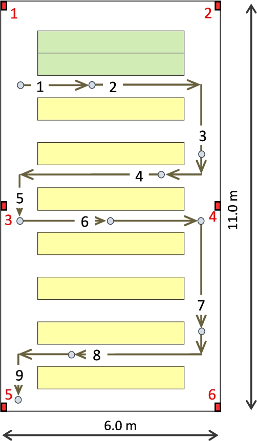
Fig. 12.

Localization accuracy for all analyzed localization algorithms at all test points.

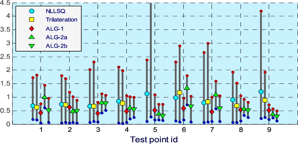
For each test point, the value of the minimum (blue dots), the maximum (red dots), and the average (different marker) of localization accuracy for each of the localization algorithms is obtained. The average localization accuracy of the ALG-1 and ALG-2 algorithms is less than 1 m for all test points. The average accuracy of algorithm ALG-2A is over 1 m for test points 1, 6 and 7. The reason for this is that this algorithm has poor localization accuracy when the target point is near the side of the triangle the beacons form. The Trilateration algorithm gives a high localization error for test point 5, since for some of the measurements, the highest RSSI value give beacons 1, 3 and 5 that form a straight line, not a triangle.

Fig. 13.

Estimated routes vs. ideal route (dark gray).

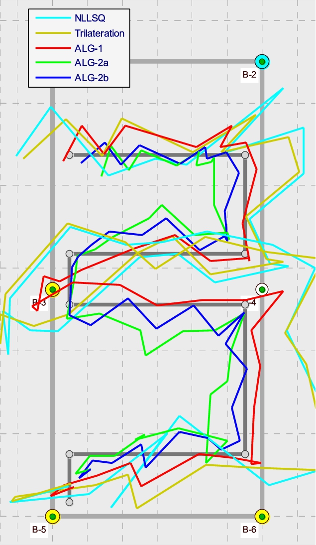
Fig. 14.

Comparison between different localization algorithms according localization precision.

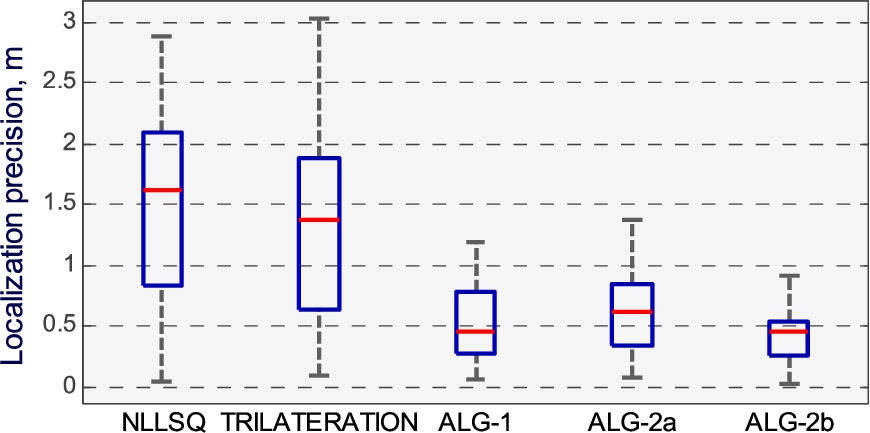
Trilateration and NLLSQ algorithms cannot be used for accurate localization, as there are measurements where the error is higher than 1 m. The best results are obtained using the ALG-2B algorithm. The next most accurate algorithm is the ALG-1.

The second experiment analyzes the localization precision of the algorithms when participants cross the route, which is formed by all test points. To compare the localization precision of the different localization algorithms, an estimate is obtained for the overall deviation from the path (the shortest distance between the calculated position and the route). Figure 13 shows the results obtained when traversing the route from test point 1 to test point 9.

The target node position is obtained every second. The length of the path is 30 m. The average time to complete this experiment is 40 seconds. The average speed of movement is 2.7 km/h. Figure 13 shows the ideal route (dark gray) and the routes obtained using each localization algorithm. The ALG-2B algorithm has the best localization precision (see Fig. 14). In this case, the deviation from the route is less than 1 m for all measurements. The next most accurate algorithm is ALG-1, for which only one measurement has a deviation greater than 1 m but less than 1.2 m. Trilateration, NLLSQ, and ALG-2A algorithms do not guarantee micro-localization.

5.Conclusions

In this article, the possibility of creating low-complexity IPS for accurate localization in smart buildings using BLE beacons is analyzed. A new adaptive algorithm for reducing noise in BLE beacon data has been proposed. The algorithm is based on a combination of a Moving Average (MA) filter and an Adaptive Kalman Filter (AKF). AKF uses fuzzy logic to estimate the noise in RSSI data and to capture visitor’s dynamics. This algorithm is designed to implement in real time. Several use case scenarios have been implemented to compare five localization algorithms. Two of these algorithms are specifically designed to be less sensitive to noise in RSSI data and require little computing power. We validate the proposed algorithms in different simulated and real building environments. The advantages and limitations for each of the algorithms are identified, based on an analysis of how their localization accuracy and precision depend on factors such as: noise level in the beacons’ data, beacons’ density, placement shape, and position of target node relative to the position of reference nodes. The following is a summary of the main results obtained after the experiments:

In a real building environment (presence obstacles for radio waves and many moving visitors) obtaining micro-localization without the use of adaptive filtering of data from beacons is not possible. The proposed data pre-processing algorithm combines MA filter and an AKF. The time to estimate the target node position is fixed to one second in order to simplify AKF calculations.
The level of fluctuations in RSSI data is 2–9 dBm and depends on a number of factors, such as distance between the beacons and multipath effect. The most dependent on noise level are the Trilateration and NLLSQ algorithms. The least noise-sensitive is ALG 2B algorithm.
The ALG-1 and ALG-2 algorithms are more sensitive than the Trilateration and NLLSD algorithms to position of the target node only if there is no noise in the RSSI data. In a real environment where there are obstacles and moving people, this is impossible. All algorithms have the highest accuracy when the target node is in the center of gravity of the shape the reference nodes form.
The density of the beacons is a major factor that affects the accuracy of all algorithms. In a real building environment, Trilateration and NLLSQ algorithms cannot be used if the distance between reference nodes d is greater than 3 m. The other algorithms guarantee accurate localization when d<10 m. Micro-localization is guaranteed when d<6 m.
The deployment shape affects the accuracy of the localization, but in a different way for the different localization algorithms. For example, the Trilateration and NLLSQ algorithms are most accurate if the shape is an equilateral or isosceles triangle. Conversely, the ALG-1 and ALG-2 algorithms are more accurate if the placement shape is rectangular.
The NLLSQ and ALG-1 algorithms can calculate the target node position using data from two or more beacons.
The choice of beacons to calculate the position of the target node should not be based solely on RSSI values. In a real environment, it is guaranteed that only the beacon with heights value of RSSI is selected correctly. For the other beacons, it should take into account what shape they form with the selected beacon. If it is necessary, the next pair of beacons should be selected.
When localizing moving objects in a real building environment, the ALG-2B algorithm has the best precision, followed by the ALG-1 algorithm.

The proposed algorithms for data pre-processing from BLE beacons and precise localization can be used in many services for visitors to smart buildings, for example: delivery of customized content depending on the location of each visitor; precise navigation of people with visual impairments in large public buildings [14]; detection of social interactions among humans [2], etc.

References

[1]	S. Alletto et al., An indoor location-aware system for an IoT-based smart museum, IEEE Internet Things J. 3: ((2016) ), 244–253. doi:10.1109/JIOT.2015.2506258.
[2]	P. Baronti et al., Remote detection of social interactions in indoor environments through bluetooth low energy beacons, J. Ambient Intell. Smart Environ. 12: ((2020) ), 203–217. doi:10.3233/AIS-200560.
[3]	D. Cannizzaro et al., A comparison analysis of BLE-based algorithms for localization in industrial environments, Electron 9: ((2020) ), 1–17.
[4]	S.S. Chawathe, Beacon placement for indoor localization using bluetooth, in: IEEE Conference on Intelligent Transportation Systems, Proceedings, ITSC, (2008) , pp. 980–985.
[5]	J. Chin, V. Callaghan and S. Ben Allouch, The Internet-of-Things: Reflections on the past, present and future from a user-centered and smart environment perspective, J. Ambient Intell. Smart Environ 11: ((2019) ), 45–69. doi:10.3233/AIS-180506.
[6]	P. Davidson and R. Piché, A survey of selected indoor positioning methods for smartphones, IEEE Communications Surveys and Tutorials 19: ((2017) ), 1347–1370. doi:10.1109/COMST.2016.2637663.
[7]	R. Faragher and R. Harle, Location fingerprinting with bluetooth low energy beacons, IEEE J. Sel. Areas Commun. 33: ((2015) ), 2418–2428. doi:10.1109/JSAC.2015.2430281.
[8]	N. Fet, M. Handte and P.J. Marrón, Autonomous adaptation of indoor localization systems in smart environments, J. Ambient Intell. Smart Environ. 9: ((2017) ), 7–20. doi:10.3233/AIS-160416.
[9]	C. Gomez, S. Chessa, A. Fleury, G. Roussos and D. Preuveneers, Internet of Things for enabling smart environments: A technology-centric perspective, J. Ambient Intell. Smart Environ. 11: ((2019) ), 23–43. doi:10.3233/AIS-180509.
[10]	D.E. Grzechca, P. Pelczar and L. Chruszczyk, Analysis of object location accuracy for iBeacon technology based on the RSSI path loss model and fingerprint map, Int. J. Electron. Telecommun. 62: ((2016) ), 371–378. doi:10.1515/eletel-2016-0051.
[11]	W. He, P.H. Ho and J. Tapolcai, Beacon deployment for unambiguous positioning, IEEE Internet Things J. 4: ((2017) ), 1370–1379. doi:10.1109/JIOT.2017.2708719.
[12]	K.E. Jeon, J. She, P. Soonsawad and P.C. Ng, BLE beacons for Internet of things applications: Survey, challenges, and opportunities, IEEE Internet of Things Journal 5: ((2018) ), 811–828. doi:10.1109/JIOT.2017.2788449.
[13]	Z. Kaibi, Z. Yangchuan and W. Subo, Research of RSSI indoor ranging algorithm based on Gaussian – Kalman linear filtering, in: Proceedings of 2016 IEEE Advanced Information Management, Communicates, Electronic and Automation Control Conference, IMCEC 2016, (2016) , pp. 1628–1632.
[14]	H.K. Lu, P.C. Lin, K.C. Chu, A.N. Chen and A. Yuan, Development and evaluation of a beacon-based indoor positioning and navigating system for the visually impaired, J. Intell. Fuzzy Syst. 37: ((2019) ), 4665–4675. doi:10.3233/JIFS-179301.
[15]	X. Luo, W.J. O’Brien and C.L. Julien, Comparative evaluation of Received Signal-Strength Index (RSSI) based indoor localization techniques for construction jobsites, Adv. Eng. Informatics 25: ((2011) ), 355–363. doi:10.1016/j.aei.2010.09.003.
[16]	A. Mackey, P. Spachos, L. Song and K.N. Plataniotis, Improving BLE beacon proximity estimation accuracy through Bayesian filtering, IEEE Internet Things J. 7: ((2020) ), 3160–3169. doi:10.1109/JIOT.2020.2965583.
[17]	F. Mekelleche and H. Haffaf, Classification and comparison of range-based localization techniques in wireless sensor networks, J. Commun. 12: ((2017) ), 221–227.
[18]	G.M. Mendoza-Silva, J. Torres-Sospedra and J. Huerta, A meta-review of indoor positioning systems, Sensors (Switzerland) 19 (2019).
[19]	J. Park, J. Kim and S. Kang, BLE-based accurate indoor location tracking for home and office, Computer Science & Information Technology (2015), 173–181.
[20]	V.C. Paterna, A. Calveras Augé, J. Paradells Aspas and M.A. Pérez Bullones, A bluetooth low energy indoor positioning system with channel diversity, weighted trilateration and Kalman filtering, Sensors (Basel) 17 (2017).
[21]	S. Pradhan, Y. Bae, J.Y. Pyun, N.Y. Ko and S.S. Hwang, Hybrid toa trilateration algorithm based on line intersection and comparison approach of intersection distances, Energies 12: ((2019) ), 1668–1694. doi:10.3390/en12091668.
[22]	U.M. Qureshi, Z. Umair and G.P. Hancke, Evaluating the implications of varying bluetooth low energy (BLE) transmission power levels on wireless indoor localization accuracy and precision, Sensors (Switzerland) 19: ((2019) ), 1–28.
[23]	J. Rezazadeh, M. Moradi, A.S. Ismail and E. Dutkiewicz, Superior path planning mechanism for mobile beacon-assisted localization in wireless sensor networks, IEEE Sens. J. 14: ((2014) ), 3052–3064. doi:10.1109/JSEN.2014.2322958.
[24]	J. Rezazadeh, R. Subramanian, K. Sandrasegaran, X. Kong, M. Moradi and F. Khodamoradi, Novel iBeacon placement for indoor positioning in IoT, IEEE Sens. J. 18: ((2018) ), 10240–10247. doi:10.1109/JSEN.2018.2875037.
[25]	L. Ruan, L. Zhang, F. Cheng and Y. Long, The global optimal placement of ble beacon for localization based on indoor map, in: International Archives of the Photogrammetry, Remote Sensing and Spatial Information Sciences – ISPRS Archives, Vol. 42: , (2018) , pp. 591–595.
[26]	S. Sadowski and P. Spachos, RSSI-based indoor localization with the Internet of Things, IEEE Access 6: ((2018) ), 30149–30161. doi:10.1109/ACCESS.2018.2843325.
[27]	S. Sadowski and P. Spachos, Optimization of BLE beacon density for RSSI-based indoor localization, in: 2019 IEEE International Conference on Communications Workshops, ICC Workshops 2019 – Proceedings, (2019) .
[28]	O.B. Sezer, E. Dogdu and A.M. Ozbayoglu, Context-aware computing, learning, and big data in Internet of Things: A survey, IEEE Internet of Things Journal 5: ((2018) ), 1–27. doi:10.1109/JIOT.2017.2773600.
[29]	E.Q. Shahra, T.R. Sheltami and E.M. Shakshuki, A comparative study of range-free and range-based localization protocols for wireless sensor network: Using COOJA simulator, Int. J. Distrib. Syst. Technol. 8: ((2017) ), 1–16. doi:10.4018/IJDST.2017010101.
[30]	P. Spachos, I. Papapanagiotou and K.N. Plataniotis, Microlocation for smart buildings in the era of the Internet of things: A survey of technologies, techniques, and approaches, IEEE Signal Process. Mag. 35: ((2018) ), 140–152. doi:10.1109/MSP.2018.2846804.
[31]	P. Spachos and K. Plataniotis, BLE beacons in the smart city: Applications, challenges, and research opportunities, IEEE Internet Things Mag. 3: ((2020) ), 14–18. doi:10.1109/IOTM.0001.1900073.
[32]	F. Zafari, A. Gkelias and K.K. Leung, A survey of indoor localization systems and technologies, IEEE Commun. Surv. Tutorials 21: ((2019) ), 2568–2599. doi:10.1109/COMST.2019.2911558.
[33]	F. Zafari and I. Papapanagiotou, Enhancing iBeacon based micro-location with particle filtering, in: 2015 IEEE Global Communications Conference, GLOBECOM 2015, (2015) , pp. 1628–1632.
[34]	Y. Zhuang, J. Yang, Y. Li, L. Qi and N. El-Sheimy, Smartphone-based indoor localization with bluetooth low energy beacons, Sensors (Switzerland) 16 (2016).