Effectiveness of deep learning techniques in TV programs classification: A comparative analysis

3.1Materials

In this section, we’re going to introduce the two methods we have developed for classifying television broadcasts and extended videos. Our goal is to pro-vide an in-depth explanation of the methodologies we’ve utilized throughout the classification process. We’ll delve into the specifics of each method, spot-lighting their distinctive features and the fundamental principles upon which they’re based. This thorough analysis will clarify the two separate strategies, set ting the stage for an exhaustive evaluation of their efficiency and their ability to adapt to different scenarios. This level of detailed scrutiny is essential to pinpoint the most appropriate and effective approach for categorizing television content and longer video formats.

We created an initial dataset for the SSIM-CNN framework. We used a first dataset comprising test images to evaluate the SSIM [14]. Originally, the images in our dataset captured the opening and closing acronymous of a sports news program. We have since expanded this dataset to include content from additional programs beyond sports, incorporating various categories from a second dataset created for CNN. To train CNN network, we assembled datasets using image annotations sourced from web search engines and video frame captures from the specified channels. The project’s initial phase concentrated on identifying content from sports news. We later expanded our dataset to include a wider range of categories. The training dataset now covers diverse genres: Geo documentaries (826 images), Religious events (769 images), Game shows (525 images), Talk shows (685 images), Sales promotions (470 images).

For our second initiative, the Shot Boundary Detection with Transformers framework, we have developed an enriched dataset of mini videos. These were generated utilizing Shot Boundary Detection techniques and were systematically classified into diverse categories following the A.g.Com program classification guidelines. This comprehensive dataset includes the following segments: Cartoons (559); Cooking (313); Culture (244); Debates (164); Religious (309); Geography (439); Interviews (476); Weather (337); Politics (100); Commercials (604); News Summaries (570); Sports(122); also integrating videos from UCF-101 [15] from specific categories due to data scarcity, particularly Basketball(15), Soccer(8), Tennis(15), Swimming(26), Golf(12), chosen based on the monitoring of the channels and the creation of the dataset itself, Teleshopping (450), and News bulletins (191).

3.2Similarity structure index measure with convolutional neural network

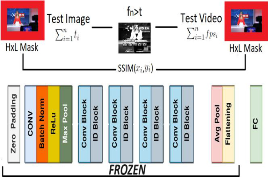
The proposed architecture utilizes an image comparison system based on SSIM, augmented with a ResNet50 [16]. This novel method focuses on analyzing stacked frames from the target video. Each frame undergoes a detailed comparison against standardized test images obtained from the broadcasting channels of the TV shows in question.

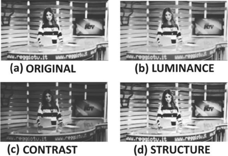
The Structural Similarity Index Measure (SSIM) [17] works as a perceptual tool quantifying image quality degradation by measuring changes in structural in-formation. Unlike most image quality metrics, which typically calculate discrepancies based on pixel value differences like mean squared error, the SSIM index reflects the human visual system’s ability to detect structural information within a scene. It excels at discerning the details between a reference image and a comparison image. A metric that mimics this capability generally excels in tasks that require this level of discrimination. The SSIM index evaluates three essential characteristics of an image: Luminance, Contrast, and Structure, as shown in Fig. 1.

Figure 1.

Comparative visualization of the SSIM metrics: Original, Luminance, Contrast, and Structure.

Consider a collection of test images; every image is represented as a Matrix I that capture specific moments of detection, such as the beginning or the end of a TV show’s acronym. Each image has size N⋅ N, and we define with n the n-th image {I⁢1,I⁢2,I⁢3,…,I⁢n}.

A video is essentially a temporal sequence of images, each always represented as a matrix Mi where i indicates the frame number over time. If the video consists of n frames, then we have a set of matrices {M⁢1,M⁢2,…,M⁢n}.

The goal is to precisely identify these distinct moments, like the commencement or conclusion of a TV show acronym. Under the assumption of discrete signals, Luminance is determinate by computing the average of all pixel values:

The luminance comparison function, denoted as l⁢(x,y), relies on μ⁢x and μ⁢y. In this context, x⁢i represents i-th pixel value of image x, while yi denotes the i-th pixel value of image y. The variable

N represents the total number of pixel values. Regarding contrast, it is determined by calculating the standard deviation, i.e. the square root of the variance, across all pixel values:

The contrast denoted as c⁢(x,y), involves comparing σ⁢x and σ⁢y.

In this case, x and y represent the two images under comparison, and μ is the average of the pixel values. The structural comparison is conducted by dividing the input signal by its standard deviation, which normalizes the result to a standard deviation of one, facilitating a more reliable comparison:

We define functions that compare two specified images based on these parameters. We refer to the luminance comparison function as follows:

where C1 serves as a constant to ensure stability when the denominator drops to zero. C1 is given by:

where K is a constant and L represents the dynamic range of the pixel values, which is set to 255 because we are analyzing 8-bit images. The contrast comparison function is defined as follows:

C2 shares the same structure as C1. The structure comparison function is defined as follows:

where σ⁢x represent the standard deviation of a given image, and σ⁢𝑥𝑦 pertains to the covariance of images being compared. Now, we can define the similarity index using:

The parameters γ> 0, β> 0, and α> 0 are utilized to adjust the relative prominence of the three components. By setting α=β=γ= 1, and assigning C3=C2/2, we obtain the following expression:

It is advantageous to use the SSIM index locally rather than globally for assessing the image quality. Instead of applying the metrics globally, it is more effective to apply them regionally for higher accuracy. Facing the challenge of comparing images extracted from videos, referred to as Mn, with test images, labeled In. It’s crucial to note that while the Mn video frames include specific date and time information at the time of their recording, displayed on the edges of the image, the In test images have been saved with fixed date and time stamps, corresponding to the original video from which they were extracted. This temporal discrepancy between the test images and the video frames can vary, especially if the video frames are from recordings made on different days. This difference in date and time information can lead to errors in comparisons based on the SSIM index, a metric used to assess image similarity. To address this issue, we have developed and applied a mask of H×L dimensions to both the Mn video frames and the In test images. The use of this mask allows us to exclude the date and time information from the comparison process, thereby improving the accuracy in evaluating the similarity between the images. This leads to a further reduction in image size. Regarding classification, we feed the video’s SSIM index between an old and a new scene change duration, resulting in a floating-point value SSIM (x, y)=𝑓𝑛, where the index n represents the n-th comparison between the Test image In, and the n-th frame in the Mn video.

Using a standard parameter threshold t:

By setting t to a high value, we can accurately identify when an image of interest represents a TV theme acronym. Once the image of interest is identified, CNN with ResNet50 initiates the classification of general content, including sports, human activities, sales, products, talk shows, debates, and others. For training the network, we converted the images to grayscale and employed the technique of transfer learning [18]. This involved pre-training the network on ImageNet [19]. Splitting the model into a head and body, training only the head while freezing the body. In our training data, we incorporate random rotations, zooms, shifts, shears, and flips to augment the dataset. We employed a stacked frame recognition technique: to achieve temporal classifications of scenes, we implemented a moving average prediction, by considering the frames per second of the video.

As we have represented the frames in a video as an M matrix, we define:

The ResNet50 makes predictions on each frame, assigning a classification percentage to every nth frame. Mn, we write the prediction function as:

here pn represents the probability assigned to the nth frame. We only consider the highest probabilities and can define a subset of these probabilities. Let’s assume we want to consider the top k probabilities, where k⩽N and N is the total number of frames being considered. We order the probabilities in descending order and take the first k: {p(1), p(2), …, p(k)} where p⁢(1)⩾p⁢(2)⩾…⩾p⁢(k). Let p⁢(j) denote the j^th-highest probability, after ordering all probabilities in descending order.

We now calculate the average of the top k probabilities as follows:

This value represents the overall mean probability based on the frames with the highest classification confidence of the neural network. This approach is used to evaluate the performance of the network on video segments.

Figure 2.

Architecture of SSIM with CNN.

3.3Shot boundary detection with transformer

The proposed framework operates based on optical flow. In this scenario, the video to be analyzed is divided into subsequences.

Given a video as Y, let us define Y as a sequence of frames Y={M⁢1,M⁢2,…,𝑀𝑛} where Mn represents the i-th frame of the video. With the shot boundary detection technique, we divide the video Y into n sub videos, y⁢1,y⁢2,…,𝑦𝑛, where each yk represents a video segment with a distinct semantic event. This subdivision can be expressed as: Y=⋃j=1k𝑦𝑗, where 𝑦𝑗={M𝑎𝑗,M𝑎𝑗+1,…,Mb} defining aj e bj as variables that represent the indices of the frames defining the start and end of each sub video yj with 1⩽𝑎𝑗⩽𝑏𝑗⩽n⁢e⁢𝑎𝑗+1=𝑏𝑖+1 for every i from 1 to k-1. This ensures that each frame of Y belongs to exactly one sub video yj. Each subsequence will be the input for the Transformers Network [20].

The video segmentation is realized with a shot boundary detection [21], that generates a binary mask 𝑀𝑦⁢(i,l), where i represents the vertical coordinate of the pixel. Then, l denotes the horizontal coordinate of the pixel. Representing the area of the image occupied by the foreground object. This mask is produced by applying an adaptive threshold to the difference map between the current frame 𝐼𝑦⁢(i,l) and the background model 𝐵𝑦⁢(i,l). The adaptive threshold is determined as the mean plus a constant multiplied by the standard deviation. It is specifically dependent on the standard deviation of the difference map 𝑀𝑦⁢(i,l)= 1 if:

and 0 otherwise, where μ represents the mean of the difference map, highlighting the disparity between the current frame and the background model. σ denotes the standard deviation of the difference map, while k is a multiplicative constant used to compute the adaptive threshold for generating the binary mask.

In this study, we introduce a novel video classification model that harnesses the capabilities of Transformers, a category of neural networks renowned for their proficiency in handling sequential data. The structure of our model consists of several critical components. Initially, video subsequences yj, are pre-processed by segmenting them into frames, then sub-sampled to create sequences. These sequences are subsequently processed by a DenseNet121 [22], a pre-trained convolutional neural network, to extract prominent features. The top layers of the DenseNet are excluded to maintain its expertise in capturing detailed spatial information.

Features of each frame (X ∈R𝑁𝑥𝐷) are arranged into a sequence (S ∈R𝑇𝑥𝑁𝑥𝐷), like the patch-based method used in Vision Transformers. This sequence, enhanced with positional embeddings (PE ∈R𝑇𝑥𝐷), is processed by a single layer of the Transformer. The output of the Transformer, Z, is provided by:

where S represents the sequence of features extracted from each frame of the video, organized to reflect the spatial and temporal structure of the original sequence of frames.

Figure 3.

Architecture of the shot boundary detection with transformer.

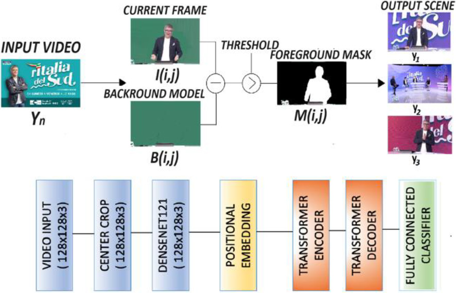
Each element of S is a feature vector describing a frame or frame segment of the video. PE represents positional embeddings, which are added to the S sequence to provide the Transformer with information about the temporal position of each frame within the sequence. This layer is designed to learn spatial and temporal dependencies among the features, providing a proficient solution for the analysis of video data. Moreover, the model makes use of a GlobalMaxPooling1D operation to effectively refine spatial information:

and this is complemented by a dropout layer to reduce the risk of overfitting.

The Transformer features a single attention head, and projects the embeddings through a dense layer with a dimensionality of 4 (F∈RTx4), thereby enhancing the model’s learning capabilities:

in essence, F represents the final processing of the input data through the Transformer model, where, after leveraging the spatial and temporal learning capabilities of the single attention head, the features are synthesized into a four-dimensional vector for each timestep. This condensed output, F, embodies the understanding gleaned by the model and is poised for deployment in decision-making stages, such as classification or advanced interpretation of patterns in video data.

4.1Performance of the proposed system

To evaluate how well the system operates, we use P to represent a favorable outcome, and N to symbolize an unfavorable one. Here’s how we classify the results: TP refers to the count of scenes accurately recognized in a video, FP is used for the count of scenes recognized in a video but labeled incorrectly, TN is the count for scenes that were misidentified in a video, and FN stands for the scenes in a video that went undetected or for any irregularities found. We paid more attention to the 2 transformer and shot boundary methodology.

The framework’s performance was carefully assessed by utilizing:

Accurately describing the results obtained.

4.2Evaluation of similarity structure index measure with ResNet50

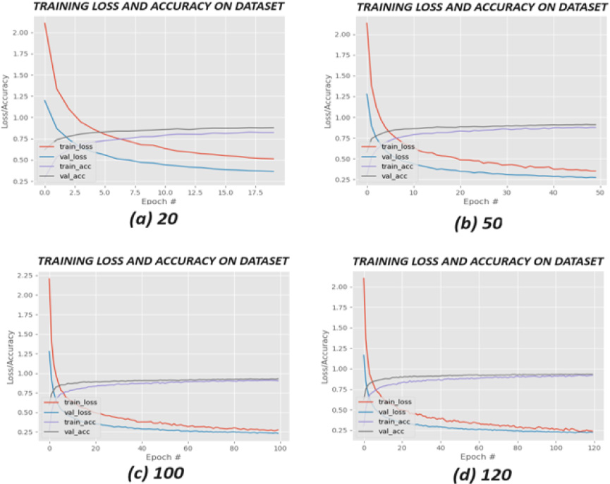
The results of the classification are shown in Table 1, which serves as an example of the results derived from the framework classification process. In this table, we can examine the first row that details the performance of SSIM, then the classification done on each framework by ResNet50. We divided the dataset, allocating 80% for training and 20% for validation. Figure 4 illustrates the training loss and accuracy of the network, employing cross-entropy to measure the difference between the model’s predictions and the actual labels throughout the training period. The network underwent training over 20, 50, 100, and 120 epochs.

Graph (a) – 20 epochs: The training loss decreases rapidly, indicating that the model is learning from the dataset effectively. Both the training and validation accuracy improve quickly, and appear to stabilize by the 20th epoch. There’s a small gap between training and validation loss, suggesting minor overfitting.

Graph (b) – 50 epochs: This graph extends to 50 epochs and shows a continued decrease in training loss. The training and validation accuracy both rise and then plateau, indicating that the model may not be gaining significant improvements from additional epochs. There’s a consistent gap between training and validation loss, but it does not appear to be widening significantly, which is positive.

Graph (c) – 100 epochs: Here, over 100 epochs, the training loss continues to decrease but at a much slower rate. The accuracy seems to have plateaued. The gap between the training and validation loss appears slightly larger compared to the 50 epochs graph, which may indicate overfitting as the model continues to learn specifics about the training data that do not generalize to the validation data.

Graph (d) – 120 epochs: Extending the training to 120 epochs, the loss and accuracy trends seem consistent with the 100 epochs graph. There’s a noticeable gap between the training and validation loss, which may suggest that the model isn’t likely to benefit from further training on the same data without adjustments or regularization to reduce overfitting.

Figure 4.

Comparison of learning curves for training and validation loss and accuracy on a dataset, with incremental epochs of 20, 50, 100, and 120.

The best results obtained for 120 epochs shown in Table 2 are discussing the results, Geo and Religious categories have high precision, recall, and F1 scores, all around 0.94 to 0.98, indicating that the model performs very well in these categories, with a balanced ability to identify relevant cases (precision) and to identify all actual cases (recall).

Game show, Talk show, and Sales promotion categories have slightly lower but still robust performance metrics, ranging from 0.92 to 0.95, which implies that the model is generally reliable in these classifications as well.

The accuracy of 0.95 suggests that the model correctly classifies 95% of the overall data, which is quite high for most applications.

Both the macro average and weighted average scores across precision, recall, and F1 are consistent at 0.94 and 0.95 respectively. The macro average treats all classes equally, while the weighted average takes the support (the number of true instances for each label) into account. High values in both suggest that the model’s performance is uniformly strong across all classes and that the model is not biased towards more frequently occurring classes.

The support for each class varies, with ‘Geo’ having the highest number of instances (206) and ‘Sales promotion’ the least (118). Despite these differences, the model’s performance is steady across classes.

In conclusion, the model demonstrates excellent and consistent performance across different categories with no significant signs of bias towards frequent categories.

4.3Evaluation of shot boundary detection with transformers

In our work, we pay special attention to the classification results obtained with this technique.

Figure 5.

Confusion matrix on 100 epochs.

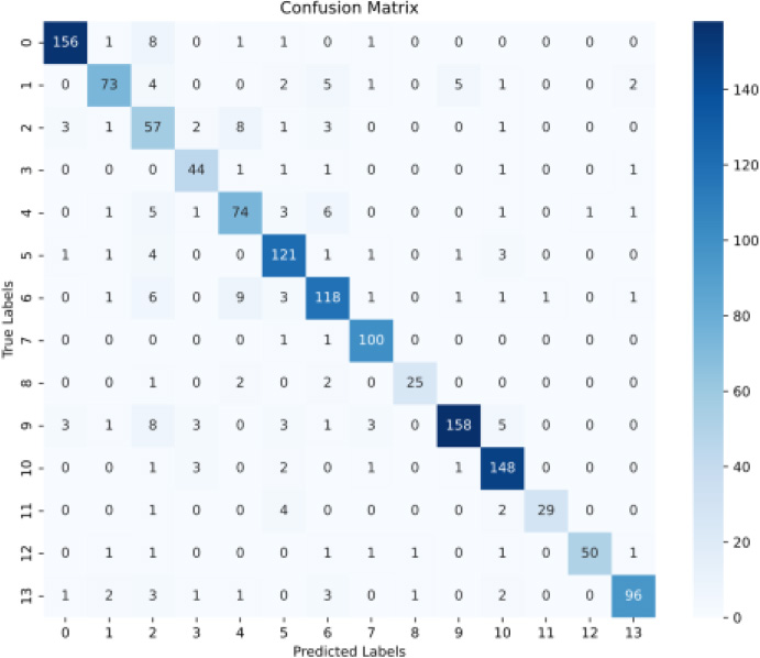
We allocated 80% of the dataset for training and the remaining 20% for testing. We conducted experiments across the different numbers of epochs at 50, 100, 150, and 200 epochs, as reported in Table 3. The best results were achieved after 100 epochs, especially when analyzing the different categories, in conjunction with the corresponding confusion matrix as illustrated in Fig. 5.

Our classification model demonstrates good results, particularly in the Cartoons and Weather categories, achieving accuracies of 0.95 and 0.92, respectively. The model’s precision in classified cartoons is confirmed by the confusion matrix, which shows 156 correct classifications out of 168 items, with very few false positives and negatives. Similarly, in the Weather category, the model correctly classified 100 out of 102 items.

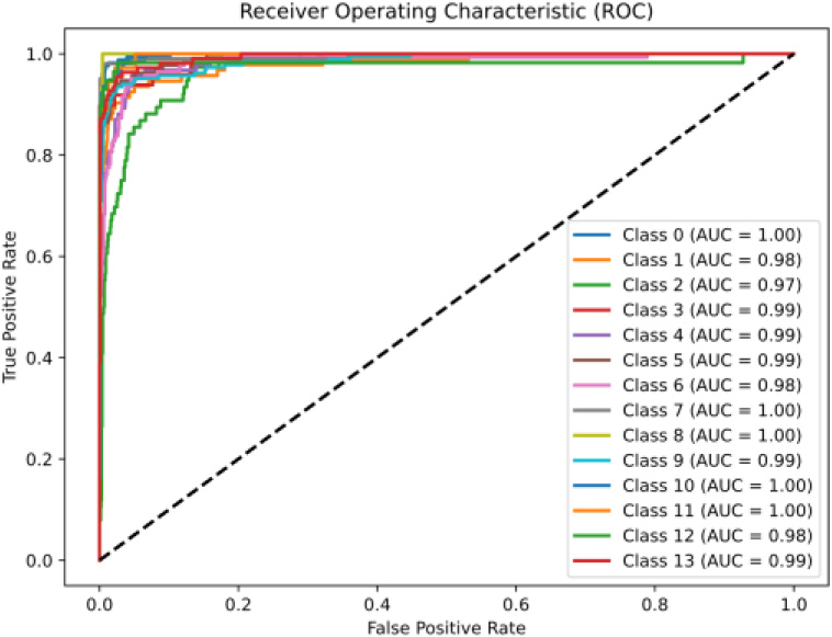
Figure 6.

ROC graphics on 100 epochs.

For Commercials and News Summaries, the model showed high accuracy, with 158 and 148 correct classifications out of 185 and 156 items, respectively. In Sports, despite a very high accuracy of 0.97, the precision is lower at 0.81, suggesting some confusion with other categories; however, the confusion matrix reveals 29 correct classifications out of 36. Teleshopping exhibits the best performance with near-perfect accuracy of 0.98 and 50 correct classifications out of 57, despite a moderate amount of misclassification indicated by the confusion matrix.

The model’s overall performance is robust with an accuracy of 0.87 across 1430 items. The macro averages for accuracy and precision, which calculate the average performance of the model for each category separately and then average these results, are 0.87 and 0.88, respectively. This indicates balanced performance across categories, ensuring that each category is given equal importance regardless of its size. Meanwhile, the weighted average, considering the number of items per category, confirms good overall performance. These results underscore the effectiveness of the model as a classification tool across a broad spectrum of categories.

Figure 6 shows the ROC (Receiver Operating Characteristic) curves over 100 epochs. These curves chart the model’s classification efficacy across 13 distinct classes by plotting the true positive rate (TPR) against the false positive rate (FPR) for various threshold settings.

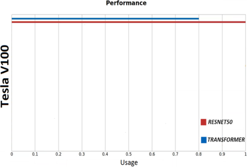
Figure 7.

GPU consumer during training of the CNN and Transformer.

The key observations from the ROC curves include:

The dashed line represents the baseline of random guessing (AUC = 0.50), with all class curves significantly outperforming this benchmark. This demonstrates that the model’s predictions are substantially superior to those made by the chance.

4.4Experimental results discussion

In this section, we provide a comparative analysis against existing research. The initial SSIM framework, when combined with a CNN, excels at quickly identifying specific TV program opening (or closing) sequence. Notably, it obviates the need for additional training when a channel updates its opening sequence; a simple test image input suffices. ResNet50 consistently shows proficiency in recognizing broader categories. However, it does come with a caveat: the alignment of the test image’s dimensions with the video’s frames per second (fps) is crucial. Conversely, the second framework, which utilizes the Transformers network for Shot Boundary Detection, adopts a more general approach to opening (or closing) sequence. Rather than focusing on individual opening sequence, it includes ‘spots’ that cover advertisements, aiming to universalize the model, thereby eliminating the need for retraining. While SSIM with ResNet50 sometimes struggles with accurately marking the beginning of TV News specifically when a journalist introduces a new report the results are generally reliable. Additionally, Fig. 7 details the GPU’s usage during training. The accompanying graph reveals that the ResNet50 network requires more power than the Transformers network. Nonetheless, it achieved remarkable results in the 120-epoch training phase, boasting an impressive 95% accuracy rate.

4.5Comparative analysis

For comparison with existing technologies, it is essential to highlight that our frameworks show promising results when benchmarked against ongoing research efforts. This underscores the potential and effectiveness of our approach amidst the current technological advancements in the field. In Table 4, we juxtapose our findings with those from recent studies in this area. For instance, in [23], the authors leverage the UCF101 dataset to classify a variety of human actions or activities in videos. Notably, their study reveals that our proposed methodologies forego the need for optical flow extraction, enhancing efficiency in terms of execution speed. Our approach utilizes a dual-stream data setup, one stream for visual inputs and another for motion, ensuring a robust representation of spatiotemporal data. It should be noted, though, that training deep neural networks like three-dimensional CNNs demands extensive data and computational power, culminating in a top accuracy of 90.2% for our Two-stream 3D network.

In [24], the researchers introduce a hybrid model that combines a Convolutional Neural Network (CNN) with a Recurrent Neural Network (RNN) to discern video content types, classifying them into categories such as ‘Animation,’ ‘Gaming,’ ‘Natural Content,’ ‘Flat Content,’ and so on. They propose a novel technique for classifying only key frames, thus curtailing processing time without significantly affecting performance. Using specific classes from the COIN dataset, they selected 1,000 images for training and testing, yielding an accuracy of 80.27%. The model’s efficacy was assessed on low-power hardware, which imposed limitations on processing capacity and necessitated the use of a smaller dataset sample.

In [25], the focus is on scene change detection within videos, using PCA in the context of identifying scene transitions. This involves extracting frames from videos and compiling them into a dataset categorized by types of content, such as journalistic reports and sports, with an accuracy of 89.3%. ResNet50 was deployed for classifying transition and non-transition frames within the training classes.

Lastly [26], presents a framework detailing the use of audio features to differentiate between types of television programming like news, sports, and entertainment. Audio data is converted into spectrograms, visual representations of frequency and time within the audio signal, which then serve as inputs for a Convolutional Neural Network (CNN) trained on Audio Set and tested on a tailored BBC dataset, coupled with a Multilayer Perceptron classifier on the backend. The CNN assesses the likelihood of specific sound events within the recording, achieving a commendable accuracy of approximately 93.7%. However, the spectrogram representation might not capture the entire spectrum of relevant audio information in television programs. Despite the inclusion of broadcasts from various genre categories, there’s a possibility that some genres are overrepresented relative to others. In [27], the focus is on classifying violent content in videos using deep neural networks (DNNs) trained on the VSD2014 benchmark, which differentiates between violence and non-violence. The highest accuracy achieved was 53% with a network consisting of 21 hidden layers, implemented on a MacBook Pro. The experimental findings suggest that all the various architectures of hidden layers and nodes explored did not surpass 57% accuracy, warranting further research.

In [28], the authors explore and compare different methodologies for the challenging task of classifying television programs. Logistic Regression emerged as the most effective, boasting an 82% accuracy for newly classified content. This method has proven its merit, particularly in scenarios involving brief documents and a limited number of training samples. The principal limitation identified in the study is that despite certain enhancements, incorporating semantic information from Wikipedia did not significantly improve the accuracy of television program classification. In [29] contribute to the ongoing research discourse, as presented at the the European Conference on Advances in Databases and Information Systems in 2023. It introduces various methodologies for the classification of television programming.

References

[1] | Agcom.2008, Available from: https://wwwagcom, it/ documents/10179/539063/Allegato+12-11-2008+13. |
[2] | Candela F, Morabito FC, Zagaria CF. Television programs classification via deep learning approach using SSMI-CNN. In: Proceedings of the Second International Conference on Applied Intelligence and Informatics (AII 2022). (2022) Sep 1–3; 293-307. Cham, Switzerland. Springer. 2023. |
[3] | Tran D, Bourdev L, Fergus R, Torresani L, Paluri M. Learning spatiotemporal features with 3D convolutional networks. In: Proceedings of the IEEE International Conference on Computer Vision. (2015) ; 4489-4497. |
[4] | Simonyan K, Zisserman A. Two-stream convolutional networks for action recognition in videos. In: Advances in Neural Information Processing Systems. (2014) ; 27. |
[5] | Wang L, Xiong Y, Wang Z, Qiao Y. Temporal segment networks: Towards good practices for deep action recognition. In: Proceedings of the European Conference on Computer Vision (ECCV). (2016) . |
[6] | Carreira J, Zisserman A. Quo vadis, action recognition? A new model and the kinetics dataset. In: Proceedings of the IEEE Conference on Computer Vision and Pattern Recognition. (2017) ; 4724-4733. |
[7] | Feichtenhofer C, Fan H, Malik J, He K. SlowFast networks for video recognition. In: Proceedings of the IEEE/CVF International Conference on Computer Vision. (2019) ; 6202-6211. |
[8] | Bahdanau D, Cho K, Bengio Y. Neural machine translation by jointly learning to align and translate. arXiv preprint arXiv1409.0473. |
[9] | Sharma S, Kiros R, Salakhutdinov R. Action recognition using visual attention. arXiv preprint arXiv1511.04119. |
[10] | Hu W. IEEE transactions on systems, man, and cybernetics – part c: Applications and reviews. (2011) ; 41: (6): 729-743. |
[11] | Cao Y, Qiu M, Feng W, Li J. Scene-based TV program classification with visual attention mechanism. In: 2019 IEEE International Conference on Multimedia and Expo (ICME). (2019) ; 640-645. doi: 10.1109/ICME.2019.00230. |
[12] | Wu F, Zuo L, Chen S, Tang Y. TV program classification with multi-modality features and multi-task learning. In: 2020 IEEE International Conference on Multimedia and Expo (ICME). (2020) ; 1-6. doi: 10.1109/ICME46284.2020.9102761. |
[13] | Le HK, Moon S. Automatic TV program genre classification using deep convolutional neural networks. In: Proceedings of the 16th International Conference on Control, Automation, Robotics and Vision (ICARCV). (2019) ; 133-138. IEEE. |
[14] | Candela F. SSIM_PROGRAM_CLASSIFICATION. Available from: https://githubcom/itsCandels/SSIM_PROGRAM_CLASSIFICATION-main. |
[15] | Soomro K, Zamir AR, Shah M. UCF101: A dataset of 101 human actions classes from videos in the wild. arXiv preprint arXiv1212.0402. |
[16] | He K, Zhang X, Ren S, Sun J. Deep residual learning for image recognition. In: Proceedings of the IEEE Conference on Computer Vision and Pattern Recognition. (2016) ; 770-778. |
[17] | Wang Z, Bovik AC, Sheikh HR, Simoncelli EP. Image quality assessment: From error visibility to structural similarity. IEEE Transactions on Image Processing. (2004) ; 13: (4): 600-612. |
[18] | Krizhevsky A, Sutskever I, Hinton GE. ImageNet classification with deep convolutional neural networks. In: Advances in Neural Information Processing Systems 25 (NIPS 2012). (2012) ; 1097-1105. |
[19] | Deng J, Dong W, Socher R, Li LJ, Li K, Fei-Fei L. Imagenet: A large-scale hierarchical image database. In: Proceedings of the 2009 IEEE Conference on Computer Vision and Pattern Recognition. IEEE. (2009) ; 248-255. |
[20] | Vaswani A, Shazeer N, Parmar N, Uszkoreit J, Jones L, Gomez AN, et al. Attention is all you need. In: Advances in Neural Information Processing Systems. (2017) ; 30. |
[21] | Jadhav DA, Sharma Y, Arora PS. Adaptive background subtraction models for shot detection. In: Advances in Signal and Data Processing: Select Proceedings of ICSDP 2019. Springer Singapore. (2021) . |
[22] | Huang G, Liu Z, Van Der Maaten L, Weinberger KQ. Densely connected convolutional networks. In: Proceedings of the IEEE Conference on Computer Vision and Pattern Recognition. (2017) ; 4700-4708. |
[23] | Diba A, Pazandeh AM, Van Gool L. Efficient two-stream motion and appearance 3D CNNs for video classification. arXiv preprint arXiv1608.08851. |
[24] | Patil P, Saitwal K, Kamat P, Kulkarni A. Video content classification using deep learning. arXiv preprint arXiv2111.13813. |
[25] | Chakraborty D, Chiracharit W, Chamnongthai K. Video shot boundary detection using principal component analysis (PCA) and deep learning. In: 2021 18th International Conference on Electrical Engineering/Electronics, Computer, Telecommunications and Information Technology (ECTI-CON). IEEE. (2021) ; 272-275. |
[26] | Pham L, Tran D, Nguyen D, Phan S. An audio-based deep learning framework for BBC television program classification. In: 2021 29th European Signal Processing Conference (EUSIPCO). IEEE. (2021) . |
[27] | Ali A, Senan N. Violence video classification performance using deep neural networks. In: Recent Advances on Soft Computing and Data Mining: Proceedings of the Third International Conference on Soft Computing and Data Mining (SCDM 2018). Springer International Publishing. (2018) ; 91-100. |
[28] | Narducci F, Musto C, Semeraro G, Lops P, de Gemmis M. TV-program retrieval and classification: A comparison of approaches based on machine learning. Information Systems Frontiers. (2018) ; 20: : 1157-1171. |
[29] | Candela F. Deep learning techniques for television broadcast recognition. In: European Conference on Advances in Databases and Information Systems. Cham: Springer Nature Switzerland. (2023) . |
[30] | Rafiei MH, Adeli H. A new neural dynamic classification algorithm. IEEE Transactions on Neural Networks and Learning Systems. (2017) ; 28: (12): 3074-3083. doi: 10.1109/TNNLS.2017.2682102. |
[31] | Alam KMR, Siddique N, Adeli H, Rafiei MH, Gauthier L, Takabi D. Self-supervised learning for electroencephalography. IEEE Transactions on Neural Networks and Learning Systems. (2023) . |