
An Improved Algorithm for Extracting Frequent Gradual Patterns
Abstract
Frequent gradual pattern extraction is an important problem in computer science widely studied by the data mining community. Such a pattern reflects a co-variation between attributes of a database. The applications of the extraction of the gradual patterns concern several fields, in particular, biology, finances, health and metrology. The algorithms for extracting these patterns are greedy in terms of memory and computational resources. This clearly poses the problem of improving their performance. This paper proposes a new approach for the extraction of gradual and frequent patterns based on the reduction of candidate generation and processing costs by exploiting frequent itemsets whose size is a power of two to generate all candidates. The analysis of the complexity, in terms of CPU time and memory usage, and the experiments show that the obtained algorithm outperforms the previous ones and confirms the interest of the proposed approach. It is sometimes at least 5 times faster than previous algorithms and requires at most half the memory.
1Introduction
The technological development in the last decades has allowed the creation of many electronic devices used to solve the current problems of humanity. These devices are present in many aspects of human life such as health, agriculture, economy and education. They produce and store huge amounts of digital data, which in turn contain a certain amount of hidden knowledge. Knowledge extraction (Di-Jorio et al., 2009a; Vera et al., 2020; Al-Jammali, 2023) aims to extract useful and understandable hidden knowledge, such as correlation, dependence or co-variation of attributes, from large databases.
A well known data mining task is frequent itemset mining, widely studied by the data mining community. It consists of analysing data to discover frequently co-occurring itemsets (Agrawal and Srikant, 1994; Kenmogne, 2018). It has many applications in many areas such as market basket analysis, e-learning, image classification, activity monitoring, community discovery, malware detection, web mining, chemical and biological analysis, and software bug analysis. Over the past decades, many studies have been devoted to frequent sequence mining (Kenmogne, 2016; Belise et al., 2017, 2018; Kenmogne et al., 2022), which generalizes frequent itemset mining by taking the sequential ordering of itemsets in transactions into account to find frequently co-occurring subsequences in a set of transactions. Recently, gradual patterns that model frequent co-variations between numerical attributes aroused great interest in a multitude of areas. They convey knowledge of the form «the more A, the more B». Examples of gradual patterns extracted from a salary database and a medical database are «the higher the age, the higher the salary» and « patients with high insulin levels, high body mass index and high age have a high probability of having diabetes», respectively. Previous studies have developed two basic algorithms for extracting frequent gradual patterns, namely Graank and Grite. Both algorithms are based on the Apriori principle, which consists in generating candidates and selecting those that are frequent. The difference between them comes from how to calculate the gradual supports. In the Grite algorithm, gradual support is based on the so-called precedence graph approach. In the Graank algorithm, it relies instead on the so-called concordant pairs approach.
Even though the problem of knowledge extraction has been addressed for many years (Frawley et al., 1992; Agrawal and Srikant, 1994; Hüllermeier, 2002; Berzal et al., 2007; Di-Jorio et al., 2009a; Kononenko and Bevk, 2009; Ayouni et al., 2010; Negrevergne et al., 2014; Kenmogne, 2016; Jabbour et al., 2019; Chicco and Jurman, 2020; Lonlac et al., 2020; Lonlac and Nguifo, 2020; Vera et al., 2020; Clémentin et al., 2021; Li and Liu, 2021; Ham et al., 2022), knowledge mining algorithms are well known to be both time and memory intensive for large databases, and the improvements are driven by the need to process more data at faster speed with less cost. This paper follows this trend for the extraction of frequent gradual patterns.
Interesting gradual pattern mining algorithms can be classified into four categories. The first category focuses on the extraction of frequent gradual patterns (Di-Jorio et al., 2009a, 2009b, 2009c; Laurent et al., 2009; Clémentin et al., 2021). The second category focuses on reducing the number of frequent gradual patterns by considering only closed or maximal patterns (Ayouni et al., 2010; Côme and Lonlac, 2021; Belise et al., 2023). The third category focuses on leveraging parallel architectures to speed up the mining process (Laurent et al., 2010, 2012; Negrevergne et al., 2014; Belise et al., 2018). The fourth category concerns the integration of constraints, related to the application context, in the mining process (Belise, 2011; Kenmogne, 2016; Belise et al., 2017; Kenmogne, 2018; Ser et al., 2018; Lonlac et al., 2020). Many algorithms of the four categories are based on the Apriori principle, also known as the test-generation principle, which consists in generating candidate itemsets, calculating their gradual supports and retaining only those candidates whose support is above the minimum threshold. In these algorithms, frequent gradual patterns of size k are used to generate candidates of size
The work presented in this paper is related to the first category of algorithms. In this category, performance optimization involves reducing the search space and reducing the costs of fundamental operations used in the mining process, namely support calculation, candidate generation and binary matrix multiplication. In mining algorithms, the search space could be reduced to the lattice of positive gradual patterns, i.e. patterns whose first term is positive. This halves the search space, which in turn results in a halving of the computational load. The reduction of support calculation costs has been studied in the literature in the particular case where the gradual support is based on the so-called precedence graph approach. This paper focuses on reducing the costs of generating and processing candidates, assuming that gradual support relies on the so-called concordant pairs approach. This results in a new approach for extracting frequent gradual patterns. Compared to previous approaches, the cost of candidate generation is significantly reduced by using only frequent gradual itemsets whose size is a power of two to generate all candidates. More precisely, frequent gradual patterns of size
The rest of the paper is organized as follows. Section 2 presents related work. Section 3 presents a new approach for the extraction of frequent gradual patterns. Section 4 presents the experimental results. Section 5 concludes the paper.
2State of the Art
This section presents the fundamental concepts of the extraction of the gradual patterns and the methods of extraction of the said patterns.
2.1Concepts and Definitions
The database described in Table 1 is used to illustrate the concepts and methods for extracting gradual patterns.
Table 1
Example of a numerical database
| Id | Age (A) | Salary (S) | Car (C) |
| 22 | 1200 | 0 | |
| 28 | 1850 | 2 | |
| 24 | 1200 | 3 | |
| 35 | 2200 | 1 |
Definition 1
Definition 1(Item).
An item is an attribute of the database.
For example, in Table 1, A, S and C are items.
Definition 2
Definition 2(Gradual Item).
A gradual item is of the form
In database
Definition 3
Definition 3(Gradual pattern or gradual itemset).
A gradual pattern M, also called gradual itemset, is a concatenation of several gradual items, denoted
M is linguistically interpreted as a conjunction of gradual items. A k-gradual itemsets is an gradual itemset containing k gradual items. For example, the 2-gradual itemset
Definition 4
Definition 4(Complementary gradual itemset).
Let
In the literature, it is often assumed that
Definition 5
Definition 5(Gradual rule).
A gradual rule, denoted R:
The rule
Definition 6
Definition 6(Concordant pairs).
A concordant pair with respect to a gradual itemset is a pair of objects in the database that satisfies the order induced by the said itemset.
For example,
Definition 7
Definition 7(Binary matrix of an itemset, Di-Jorio et al., 2009a).
Let
Table 2 illustrates the notion of binary matrix of a gradual itemset and the calculation of the binary matrix of a concatenation of itemsets. If
Table 2
Binary matrices of some itemsets from database
| ↱ | ||||||||||||
| 0 | 1 | 1 | 1 | 0 | 1 | 0 | 1 | 0 | 1 | 1 | 1 | |
| 0 | 0 | 0 | 1 | 0 | 0 | 0 | 1 | 0 | 0 | 1 | 0 | |
| 0 | 1 | 0 | 1 | 0 | 1 | 0 | 1 | 0 | 0 | 0 | 0 | |
| 0 | 0 | 0 | 0 | 0 | 0 | 0 | 0 | 0 | 1 | 1 | 0 | |
| ↱ | ||||||||||||
| 0 | 1 | 0 | 1 | 0 | 1 | 1 | 1 | 0 | 1 | 0 | 1 | |
| 0 | 0 | 0 | 1 | 0 | 0 | 0 | 0 | 0 | 0 | 0 | 0 | |
| 0 | 1 | 0 | 1 | 0 | 0 | 0 | 0 | 0 | 0 | 0 | 0 | |
| 0 | 0 | 0 | 0 | 0 | 0 | 0 | 0 | 0 | 0 | 0 | 0 | |
Proposition 1
Proposition 1(Binary matrix of a complementary itemset).
If
The extraction of the relevant gradual patterns and rules is based on quality criteria that are based on the concept of support and the concept of trust. The definition of the support concept varies depending on the extraction method. This paper considers the definition based on the notion of concordant pairs.
Definition 8
Definition 8(Support of a gradual pattern, Berzal et al., 2007).
The support
(1)
Table 3 illustrates the notion of gradual support.
Table 3
Gradual supports of some itemsets from database
| Itemset | Complementary itemset | List of concordant pairs | Support |
Proposition 3.
If a gradual pattern is frequent then its complementary is also frequent.
Proposition 3 is a consequence of Proposition 2.
Definition 9
Definition 9(Confidence of a gradual rule).
The confidence
(2)
Definition 10
Definition 10(Frequent gradual pattern).
A gradual pattern M is said to be frequent if its support is greater than or equal to the minimum support threshold minSupp, i.e.
Definition 11
Definition 11(Valid gradual rule).
A gradual rule R is said to be valid if its confidence is greater than or equal to the minimum confidence threshold minCon, i.e.
2.2Some Approaches to Extracting Gradual Itemsets
The first approach is based on the notion of linear regression (Hüllermeier, 2002). It only considers fuzzy data and rules whose premise and conclusion have a size less than or equal to two. However, the notion of T-norm makes it possible to overcome the size limitation of the premises and conclusions of the gradual rules. This approach makes it possible to extract the gradual rules.
The second approach evaluates the support of a gradual pattern as a function of the number of concordant pairs and the total number of pairs in the database. The support calculation formula proposed in Berzal et al. (2007), corresponds to that of Definition 1. This definition is implemented in the Graank algorithm (Laurent et al., 2009), which extracts frequent gradual patterns. However, in some works, instead of considering half of the total number of pairs in the database, the total number of pairs in the database is considered instead and the support formula becomes:
(3)
The third approach evaluates the support of a gradual pattern based on the longest path of its precedence graph. The nodes of the graph are the objects of the database and the arcs translate variations which are in adequacy with the set of comparison operators of the pattern. The graph of precedence of a gradual pattern is a graphic representation of its binary matrix. The Grite algorithm (Di-Jorio et al., 2009c), which extracts frequent gradual patterns, is based on this approach. Like Graank, Grite is based on the Apriori principle. Its weakness comes from the relatively high cost of calculating the longest path of a precedence graph. Therefore, the computational cost of gradual support is high compared to that of Graank. On the other hand, Graank takes into account the magnitude of the distortion for data that do not satisfy the gradual itemsets. Indeed, the deletion of an object can considerably reduce the value of the support and lead to additional calculations in the Grite algorithm.
3An Improved Algorithm
3.1Presentation of Two Versions of the Proposed Algorithms
Fig. 1
General principle of the new algorithm. In this figure
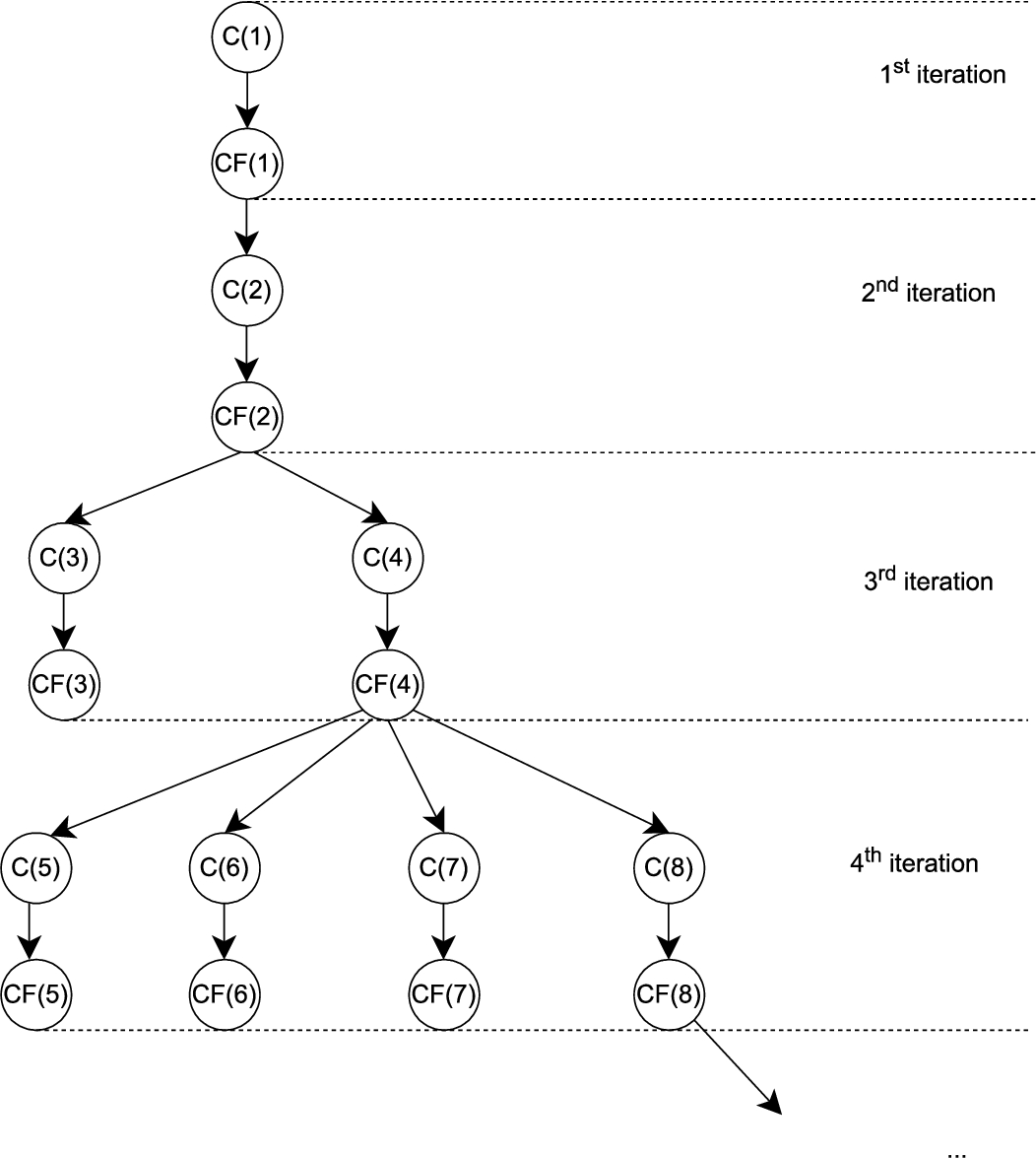
Like most pattern discovery algorithms following the Apriori principle, the Graank algorithm performs a breadth-first traversal of the search space to identify frequent gradual itemsets. In this algorithm, the generation of candidate itemsets of size
The new algorithm presented here attempts to correct Graank’s weaknesses. Compared to Graank, at iteration
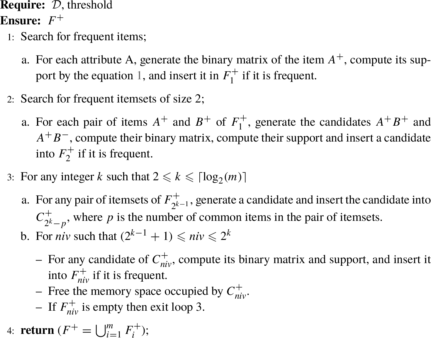
Algorithm 1
First version of the improved algorithm
Algorithm 2
Second version of the improved algorithm
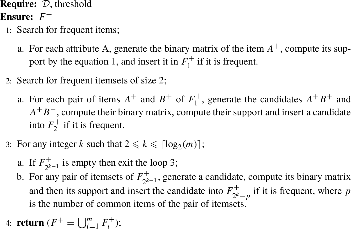
Algorithms 1 and 2 describe two versions of the improved algorithm. They take as input a database and a minimal support provided by the user, and return the set of frequent gradual patterns. Table 4 describes the list of symbols used in the algorithms. As in Graank, both versions of the proposed algorithm exploit the notion of complementarity to reduce the search space by half. To do this, only itemsets with a positive first term are handled. Both versions search and store all frequent itemsets in main memory. Both versions of the algorithm can be modified in the following way to display each frequent itemset immediately after its discovery and in such a way as to reduce the consumption of main memory:
– Display each frequent itemset after its discovery.
– Store each new frequent itemset whose size is a power of 2, i.e. of the form
– Free the memory space occupied by
There are two main differences between Algorithms 1 and 2. The first difference comes from the management of the memory space used to store the candidates of an iteration. During an iteration, Algorithm 1 generates the set of all candidates and selects the frequent ones while Algorithm 2 generates the first candidate and keeps it if it is frequent, then generates the second candidate and retains it if it is frequent, and so on. Thus Algorithm 1 requires an additional memory space to store all the candidates of each iteration while Algorithm 2 does not need such memory space. The key idea of Algorithm 2 is to save memory. The second difference comes from their termination criteria. Algorithm 1 could terminate during one iteration without computing the supports of all candidates in said iteration while Algorithm 2 cannot do this because it calculates the supports of all the candidates of an iteration. As a result, Algorithm 1 generally finishes before Algorithm 2.
Table 4
List of symbols.
| Notation | Signification |
| Database | |
| Set of frequent itemsets of sizes k whose first term is positive | |
| Set of candidate itemsets of size k whose first term is positive | |
| m | Number of database attributes |
| Threshold | Minimal support given by the user |
3.2Complexity Analysis
This section studies the time and memory complexities of Graank and the proposed algorithms.
Consider a candidate c of level
Lemma 1.
The generation of a candidate of level
Lemma 1 shows that the CPU cost of generating a candidate and computing its binary matrix is significantly improved.
Lemma 2.
Denote
(4)
(5)
Proof.
In (4) and (5), the first expression is the time complexity of the generation of candidates. The second expression is time complexity of the computation of binary matrices of candidates. □
Lemma 2 shows that, compared to Graank, the overall candidate generation runtime in the proposed algorithms is significantly improved. The overall runtime of the calculation of matrix multiplications is not improved although the execution time for the calculation of the matrix of a single itemset is significantly improved according to Lemma 1.
Denote by
(6)
This is equivalent to:
(7)
In (6), the first expression is the memory space required to store all frequent itemsets discovered between levels 1 and
In the first version of the proposed algorithm, iteration k starts by generating and storing all candidates whose size is between
(8)
This is equivalent to:
(9)
In the second version of the proposed algorithm, at iteration k, after generating a candidate whose size is between
(10)
(11)
This is equivalent to:
(12)
In formula (10), the first, second and third expressions have the same meaning as their counterpart in formula (8). The fourth expression is the memory space needed to store all frequent itemsets whose size is between
Lemma 3.
We have
Proof.
The first, second, third and fifth expression of formula (9) are respectively equal to their counterpart in formula (11). The fourth expression of formula (11) is less than its counterpart in formula (9). Thus, we have
Lemma 4.
Denote by
(13)
(14)
(15)
(16)
(17)
(18)
Proof.
(14) and (15) are straightforward from the respective definitions of
Lemma 4 shows that the first version of the proposed algorithm consumes more memory space than the second one which in turn can consume less or more memory space than Graank under certain constraints. However, the first version may stop one iteration before the second. Thus, the first version stops faster than the second. The second version stops at the start of an iteration that has no candidate. Such an iteration k implies that there is no frequent itemset of size
4Experimentations
This section compares three algorithms: Graank and two versions of the proposed algorithm. Section 4.1 presents datasets. Section 4.2 presents the results of the experimental comparisons.
4.1Presentation of Datasets
In this section, we present four types of datasets: one agricultural dataset (Islam et al., 2018), three health datasets (Li and Liu, 2021; Chicco and Jurman, 2020), one economic dataset (Clémentin et al., 2021) and three synthetic datasets (Clémentin et al., 2021).
The agricultural dataset (agricultural-dataset-bangladesh) comes from information collected on 28 agricultural areas of Bangladesh. It provides relationships between soil nutrients, types of fertilizers, types of soil and meteorological information. The soil nutrients were collected on 6 different types of land: flooded land at high altitude, flooded land at medium altitude, medium land, medium low land, flood low land, very low flood land and miscellaneous land. We have 4 types of fertilizers (urea, triple superphosphate, diammonium dhosphate, and MP). The types of soils come from 19 different types of soil and 4 different types of soil information. The meteorological data come from the Bangladesh Meteorological Department (BMD), providing information on average rainfall, maximum and minimum temperature, and humidity from 2008–2017. The complete description of the different attributes are given in Islam et al. (2018). The initial database is composed of 44 attributes and 70 transactions. For experimentation purposes, non-numeric attributes and those with missing values were remove, reducing the number of attributes to 32. The acces link to the agricultural dataset is https://www.kaggle.com/tanhim/agricultural-dataset-bangladesh-44-parameters
The three health datasets are described in the following.
1. The first health dataset concerns diabetes (diabetes.csv). It comes from the national institute of diabetes and digestive and kidney diseases. It is composed of 9 numeric attributes and 768 transactions. The objective of this dataset is to predict whether a patient is diabetic or not, based on certain diagnostic measures included in the dataset. Several constraints were placed on the selection of these instances from a larger database. In particular, all patients here are females at least 21 years old and of Pima Indian origin. The dataset is composed of several medical predictor variables and a target variable. The predictor variables include the number of pregnancies the patient has had, her BMI, insulin level, age, blood pressure, triceps skinfold thickness and diabetes pedigree function. The acces link to the diabete dataset is https://www.kaggle.com/uciml/pima-indians-diabetes-database
2. The second health dataset concerns child mortality (fetal_health.csv) (Li and Liu, 2021). These data come from Larxel Volunteer (São Paulo), It is a set of 22 numerical attributes and 2126 transactions. Due to memory limitations, only 200 transactions were considered in experimentations. The objective of this dataset is to predict fetal health allowing healthcare professionals to take action to prevent infant and maternal mortality. The different attributes in the dataset are based on Fetal Heart Rate (FHR), fetal movements, uterine contractions. The access link to the child mortality dataset is https://www.kaggle.com/andrewmvd/fetal-health-classification
3. The third and last health dataset contains medical records of 299 patients with heart failure collected at Faisalabad Heart Institute and Allied Hospital Faisalabad (Punjab, Pakistan), between April and December 2015 (heart_failure_clinical_records.csv) (Chicco and Jurman, 2020). It is a set of 13 numeric attributes and 299 transactions. The access link to this dataset is https://www.kaggle.com/andrewmvd/fetal-health-classification
The economic dataset comes from the Nasdaq Financials dataset (fundamentals.csv) (Clémentin et al., 2021). It contains 35 attributes and 300 transactions. Due to memory limitations, only the first 20 attributes and the first 150 transactions were considered in experimentations. The access link of the economic dataset is https://www.kaggle.com/dgawlik/nyse?select=fundamentals.csv.
The three synthetic datasets are C250-A100-50 (Negrevergne et al., 2014), F20Att00Li (Negrevergne et al., 2014) and test (Negrevergne et al., 2014). The access link to all these datasets is https://github.com/bnegreve/paraminer/tree/master/data/gri
The characteristics of these datasets are summarized in Table 5.
Table 5
Characteristics of the datasets.
| Datasets | Number of items | Number of transactions |
| Agricultural dataset bangladesh | 32 | 70 |
| Diabetes | 9 | 768 |
| Fetal health | 26 | 200 |
| Heart Failure Clinical Records | 13 | 299 |
| Fondamental | 20 | 150 |
| C250-A100-50 | 12 | 250 |
| F20Att200Li | 20 | 100 |
| test | 10 | 100 |
4.2Experimental Evaluation of Algorithms
This section compares the performance of the Graank algorithm (Laurent et al., 2009) and the two versions of the proposed algorithms. Experiments were performed on a computer with a Intel(R) Core(TM) i7 CPU M 620 @ 2.67 GHz 2.67 GHz with 6 GB RAM, running on Windows 10 Home 64-bit operating system. The different algorithms are implemented in Java. The purpose of experiments is to compare the runtime as depicted on Figs. 2, 3, 4, 5 and the memory consumption as shown in Figs. 6, 7, 8, 9 for different support threshold values on datasets presented on Section 4.1.
4.2.1Runtime Evaluation of Algorithms
Figure reffig:timeagriculture shows the runtime performance of the three algorithms on the agricultural dataset. The two versions of the proposed algorithm have almost similar execution times and are sometimes at least five times faster than Graank.
Fig. 2
CPU performance on agricultural dataset.
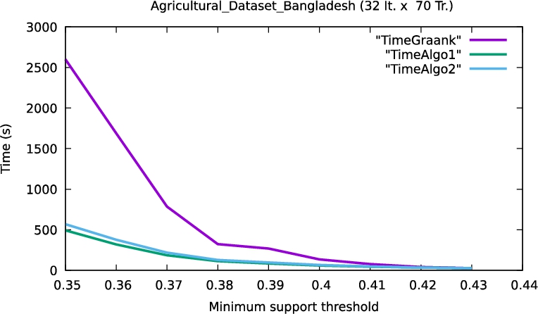
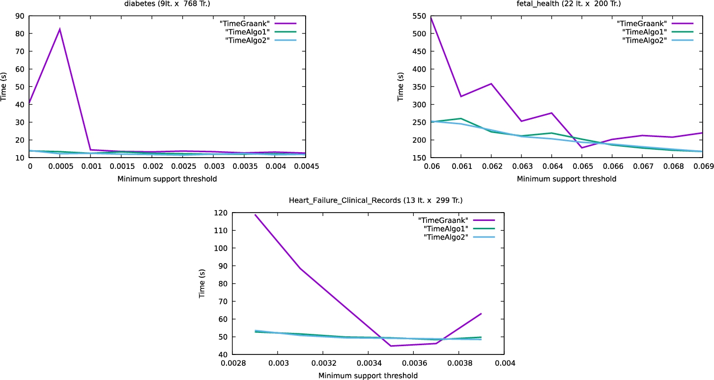
Figure 3 shows the runtime performances of the three algorithms on the three medical datasets. The two versions of the proposed algorithm are globally faster than Graank on medical datasets. Moreover, they are sometimes seven times faster than Graank on the diabete dataset and twice as fast as Graank on fetal health and heart failure datasets. However, for some support threshold values, both versions of the proposed algorithm are slightly slower than Graank. This is due to the matrix multiplication times according to Lemma 2. As with the agricultural dataset, the two versions of the proposed algorithm have nearly similar runtimes on medical datasets.
Fig. 3
CPU performance on medical datasets.
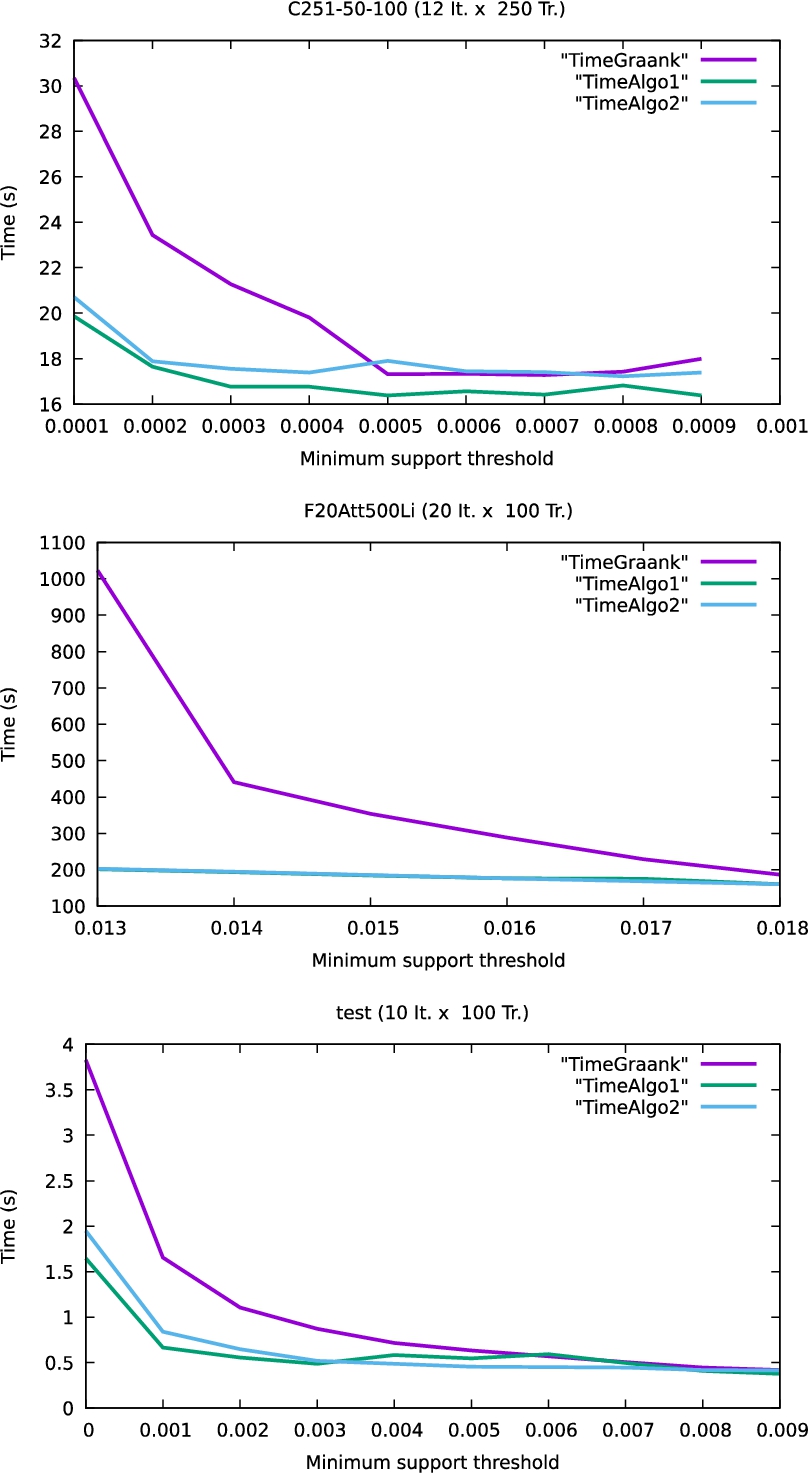
Figures 4, 5 show the runtime performances of the three algorithms on economic and synthetic datasets respectively. Both versions of the proposed algorithms are faster than Graank. On the other hand, the first version is slightly faster than the second one.
Fig. 4
CPU performance on economic dataset.
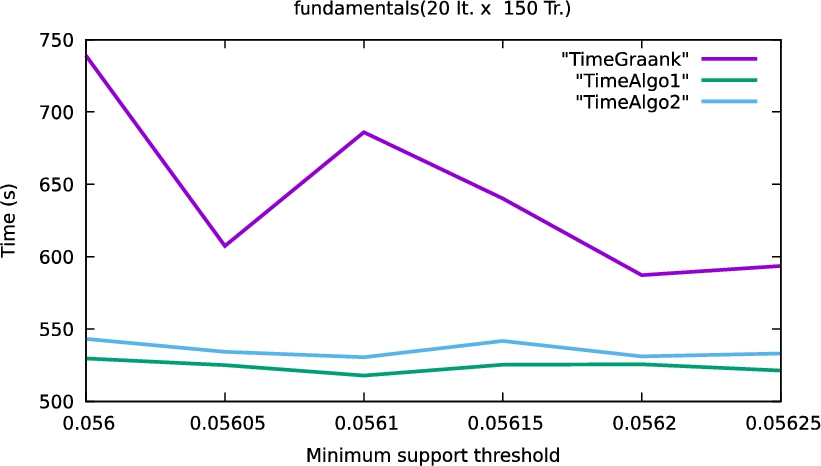
Fig. 5
CPU performance on synthetic datasets.
In summary, the runtime evaluation shows that Algorithms 1 and 2 outperform Graank in terms of CPU consumption and are sometimes at least 5–7 times faster. Between Algorithms 1 and 2, the advantage goes to Algorithm 1 in terms of CPU consumption.
4.2.2Memory Evaluation of Algorithms
Figure 6 shows the memory consumption on agricultural dataset. The memory consumption of both versions of the proposed algorithm is less than that of Graank for support threshold values which are less than 0.37 and slightly higher otherwise.
Fig. 6
RAM usage on agricultural dataset.
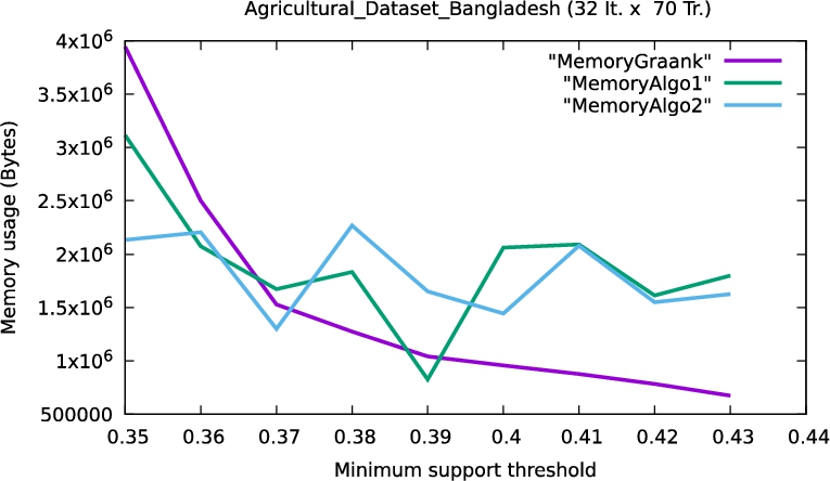
Figure 7 shows memory consumption on medical datasets. The memory consumption of both versions of the proposed algorithm is lower than that of Graank. On the other hand, the second version uses less memory than the first one.
Fig. 7
RAM usage on medical datasets.
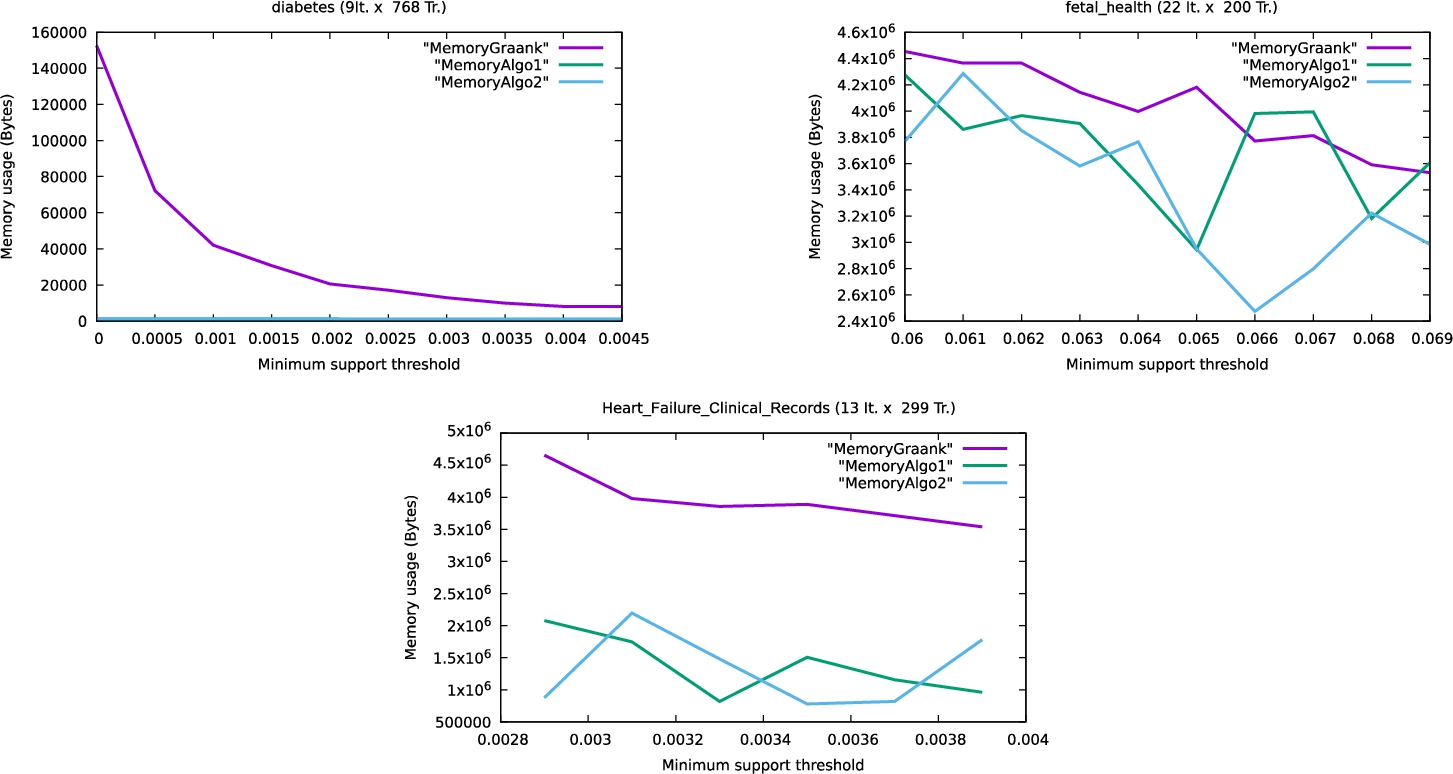
Figure 8 shows the memory consumption on the economical dataset. The memory consumption of both versions of the proposed algorithm is lower than that of Graank. Moreover, the second version uses less memory than the first one.
Fig. 8
RAM usage on economic dataset.
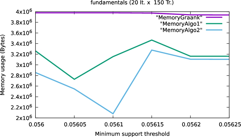
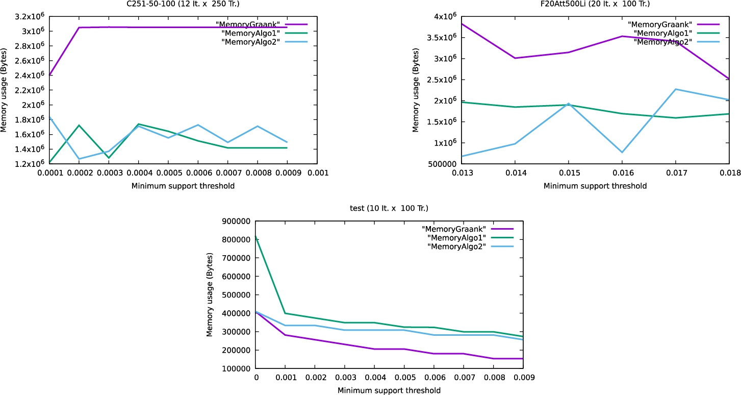
Figure 9 shows the memory consumption on synthetic datasets. The memory consumption of both versions of the proposed algorithm is lower than that of Graank on the first two datasets and slightly higher than that of Graank on the third dataset. As with the economic dataset, the second version consumes less memory than the first one.
Fig. 9
RAM usage on synthetic datasets.
In summary, the memory evaluation shows that, in general, Algorithms 1 and 2 outperform Graank in terms of memory consumption and they require sometimes at most half the memory. Between Algorithms 1 and 2, the advantage goes to Algorithm 2 in terms of memory consumption. However, there are marginal cases where Graank consumes less memory than Algorithms 1 and 2. Formula (18) in Lemma 4 characterizes some of the said cases.
4.3Presentation of Some Interesting Patterns
This section presents some interesting patterns extracted from real datasets.
4.3.1Case of the Agricultural Dataset
Here some interesting gradual patterns extracted from the agricultural-dataset-bangladesh dataset, with the minimum support threshold
4.3.2Case of Health Datasets
Here are some interesting gradual patterns extracted from the diabetes dataset with the minimum support threshold
Here are some interesting gradual patterns extracted from the fetal heart dataset with the minimum support threshold
Here are some interesting gradual patterns extracted from the heart failure dataset with the minimum support threshold
4.3.3Case of the Economic Dataset
Here are some interesting gradual patterns extracted from the fundamentals dataset, with the minimum support threshold
5Conclusion
In this paper, we have presented a new approach to improve the performance of frequent gradual pattern mining algorithms by reducing the candidate generation and processing costs. The complexity analysis and experimental performances carried out on different databases are to the advantage of the proposed approach compared to the previous ones, which confirms the effectiveness of the new approach. Sometimes, the CPU consumption gain factor is greater than 5 and the memory consumption gain factor is greater than 2. However, the theoretical and experimental studies carried out in this article reveal marginal cases for which Graank requires less memory than the proposed approach. This work opens interesting perspectives. Studying how to reduce the memory space required by Graank for marginal cases is an interesting research question. This may lead to an adaptation or improvement of the candidate generation and processing technique proposed in this paper. It could also lead to the design of a new technique. It is also interesting to study the integration of the proposed candidate generation and processing technique into other data mining algorithms in order to improve their performance. Another research question is to study how to parallelize the algorithms in which the technique proposed in this paper has been integrated in order to take advantage of the benefits offered by parallel computing for processing large datasets.
References
1 | Agrawal, R., Srikant, R. ((1994) ). Fast algorithms for mining association rules in large databases. In: International Conference On Very Large Data Bases (VLDB ‘94). Morgan Kaufmann Publishers, Inc., San Francisco, CA, USA, pp. 487–499. 1-55860-153-8. |
2 | Al-Jammali, K. ((2023) ). Prediction of heart diseases using data mining algorithms. Informatica (Slovenia), 47: (5). https://doi.org/10.31449/INF.V47I5.4467. |
3 | Ayouni, S., Yahia, S.B., Laurent, A., Poncelet, P. ((2010) ). Motifs graduels clos. In: Extraction et Gestion des Connaissances (EGC’2010), Actes, 26 au 29 janvier 2010, Hammamet, Tunisie, pp. 211–216. http://editions-rnti.fr/?inprocid=1001293. |
4 | Belise, K.E. (2011). Algorithmes des motifs séquentiels et temporels : Etat de l’art et étude comparative. Master’s thesis, Université de Dschang. |
5 | Belise, K.E., Calvin, T., Nkambou, R. ((2017) ). A pattern growth-based sequential pattern mining algorithm called prefixSuffixSpan. EAI Endorsed Transactions on Scalable Information Systems, 4: (12), 4. https://doi.org/10.4108/eai.18-1-2017.152103. |
6 | Belise, K.E., Fotso, L.C.T., Djamégni, C.T. ((2023) ). A novel algorithm for mining maximal frequent gradual patterns. Engineering Applications of Artificial Intelligence, 120: , 105939. https://doi.org/10.1016/j.engappai.2023.105939. |
7 | Belise, K.E., Roger, N., Calvin, T., Nguifo, E.M. ((2018) ). A parallel pattern-growth algorithm. In: CARI’2018, South Africa, pp. 245–256. |
8 | Berzal, F., Cubero, J.C., Sánchez, D., Miranda, M.A.V., Serrano, J. ((2007) ). An alternative approach to discover gradual dependencies. International Journal of Uncertainty, Fuzziness and Knowledge-Based Systems, 15: (5), 559–570. https://doi.org/10.1142/S021848850700487X. |
9 | Chicco, D., Jurman, G. ((2020) ). Machine learning can predict survival of patients with heart failure from serum creatinine and ejection fraction alone. BMC Medical Informatics and Decision Making, 20: (1), 1–16. |
10 | Clémentin, T.D., Cabrel, T.F.L., Belise, K.E. (2021). A novel algorithm for extracting frequent gradual patterns. Machine Learning with Applications, 5: , 100068. |
11 | Côme, A., Lonlac, J. ((2021) ). Extracting frequent (closed) seasonal gradual patterns using closed itemset mining. In: 33rd IEEE International Conference on Tools with Artificial Intelligence, ICTAI 2021, Washington, DC, USA, November 1–3, 2021. IEEE, pp. 1442–1448. https://doi.org/10.1109/ICTAI52525.2021.00229. |
12 | Di-Jorio, L., Laurent, A., Teisseire, M. ((2009) a). Extraction efficace de règles graduelles. In: Ganascia, J.-G., Gançarski, P. (Eds.), Extraction et gestion des connaissances (EGC’2009), Actes, Strasbourg, France, 27 au 30 janvier 2009. Revue des Nouvelles Technologies de l’Information, Vol. RNTI-E-15: . Cépaduès-Éditions, pp. 199–204. 978-2-85428-878-0. http://editions-rnti.fr/?procid=4591. |
13 | Di-Jorio, L., Laurent, A., Teisseire, M. ((2009) b). Mining frequent gradual itemsets from large databases. In: International Symposium on Intelligent Data Analysis, pp. 297–308. |
14 | Di-Jorio, L., Laurent, A., Teisseire, M. ((2009) c). Mining frequent gradual itemsets from large databases. In: Adams, N.M., Robardet, C., Siebes, A., Boulicaut, J.-F. (Eds.), Advances in Intelligent Data Analysis VIII, 8th International Symposium on Intelligent Data Analysis, IDA 2009, Lyon, France, August 31–September 2, 2009. Proceedings. Lecture Notes in Computer Science, Vol. 5772. Springer, pp. 297–308. 978-3-642-03914-0. |
15 | Frawley, W.J., Piatetsky-Shapiro, G., Matheus, C.J. ((1992) ). Knowledge discovery in databases: an overview. AI Magazine, 13: (3), 57–70. http://www.aaai.org/ojs/index.php/aimagazine/article/view/1011. |
16 | Ham, N., Nguyen, L., Huong, B., Tuong, L. ((2022) ). A new approach for efficiently mining frequent weighted utility patterns. Applied Intelligence, 53: (1), 121–140. https://doi.org/10.1007/s10489-022-03580-7. |
17 | Hüllermeier, E. ((2002) ). Association RUles for expressing gradual dependencies. In: Principles of Data Mining and Knowledge Discovery, 6th European Conference, PKDD 2002, Helsinki, Finland, August 19–23, 2002, Proceedings, pp. 200–211. https://doi.org/10.1007/3-540-45681-3_17. |
18 | Islam, T., Chisty, T.A., Roy, P. (2018). A Deep Neural Network Approach for Intelligent Crop Selection and Yield Prediction Based on 46 Parameters for Agricultural Zone-28 in Bangladesh. PhD thesis, BRAC University. |
19 | Jabbour, S., Lonlac, J., Saïs, L. ((2019) ). Mining gradual itemsets using sequential pattern mining. In: 2019 IEEE International Conference on Fuzzy Systems, FUZZ-IEEE 2019, New Orleans, LA, USA, June 23–26, 2019. IEEE, pp. 1–6. https://doi.org/10.1109/FUZZ-IEEE.2019.8858864. |
20 | Kenmogne, E.B. ((2016) ). The impact of the pattern-growth ordering on the performances of pattern growth-based sequential pattern mining algorithms. Computer and Information Science, 10: (1), 23–33. |
21 | Kenmogne, E.B. (2018). Contribution to the Sequential and Parallel Discovery of Sequential Patterns with an Application to the Design of e-Learning Recommenders. PhD thesis, University of Dschang. |
22 | Kenmogne, E.B., Djamegni, C.T., Nkambou, R., Tabueu Fosto, L.C., Tadmon, C. ((2022) ). Efficient mining of intra-periodic frequent sequences. Array, 16: , 100263. https://doi.org/10.1016/j.array.2022.100263. |
23 | Kononenko, I., Bevk, M. ((2009) ). Extended symbolic mining of textures with association rules. Informatica (Slovenia), 33: (4), 487–497. http://www.informatica.si/index.php/informatica/article/view/266. |
24 | Laurent, A., Lesot, M.-J., Rifqi, M. ((2009) ). GRAANK: exploiting rank correlations for extracting gradual itemsets. In: Andreasen, T., Yager, R.R., Bulskov, H., 0001, H.C., Larsen, H.L. (Eds.), Flexible Query Answering Systems, 8th International Conference, FQAS 2009, Roskilde, Denmark, October 26–28, 2009. Proceedings. Lecture Notes in Computer Science, Vol. 5822: . Springer, pp. 382–393. 978-3-642-04956-9. |
25 | Laurent, A., Negrevergne, B., Sicard, N., Termier, A. ((2010) ). PGP-mc: extraction parallèle efficace de motifs graduels. In: EGC: Extraction et Gestion des Connaissances, pp. 453–464. Cépaduès. |
26 | Laurent, A., Négrevergne, B., Sicard, N., Termier, A. ((2012) ). Efficient parallel mining of gradual patterns on multicore processors. In: Advances in Knowledge Discovery and Management. Springer, pp. 137–151. |
27 | Li, J., Liu, X. ((2021) ). Fetal health classification based on machine learning. In: 2021 IEEE 2nd International Conference on Big Data, Artificial Intelligence and Internet of Things Engineering (ICBAIE). IEEE, pp. 899–902. |
28 | Lonlac, J., Nguifo, E.M. ((2020) ). A novel algorithm for searching frequent gradual patterns from an ordered data set. Intelligent Data Analysis, 24: (5), 1029–1042. https://doi.org/10.3233/IDA-194644. |
29 | Lonlac, J., Doniec, A., Lujak, M., Lecoeuche, S. ((2020) ). Mining frequent seasonal gradual patterns. In: Song, M., Song, I., Kotsis, G., Tjoa, A.M., Khalil, I. (Eds.), Big Data Analytics and Knowledge Discovery – 22nd International Conference, DaWaK 2020, Bratislava, Slovakia, September 14–17, 2020, Proceedings. Lecture Notes in Computer Science, Vol. 12393: . Springer, pp. 197–207. https://doi.org/10.1007/978-3-030-59065-9_16. |
30 | Negrevergne, B., Termier, A., Rousset, M.-C., Méhaut, J.-F. ((2014) ). Para miner: a generic pattern mining algorithm for multi-core architectures. Data Mining and Knowledge Discovery, 28: (3), 593–633. |
31 | Ser, S., Saïs, F., Teisseire, M. ((2018) ). Découverte de motifs graduels partiellement ordonnés: application aux données d’expériences scientifiques. In: Extraction et Gestion des Connaissances, EGC 2018, Paris, France. |
32 | Vera, J.C.D., Ortiz, G.M.N., Molina, C., Vila, M.A. ((2020) ). Knowledge redundancy approach to reduce size in association rules. Informatica (Slovenia), 44: (2). https://doi.org/10.31449/inf.v44i2.2839. |


