A Deep Learning Model for Multi-Domain MRI Synthesis Using Generative Adversarial Networks

Han, Le Hoang Ngoc; Hien, Ngo Le Huy; Huy, Luu Van; Hieu, Nguyen Van

doi:10.15388/24-INFOR556

A Deep Learning Model for Multi-Domain MRI Synthesis Using Generative Adversarial Networks

Article type: Research Article

Authors: Han, Le Hoang Ngoc¹ | Hien, Ngo Le Huy² | Huy, Luu Van¹ | Hieu, Nguyen Van^{1; ∗}

Affiliations: [1] Faculty of Information Technology, The University of Danang – University of Science and Technology, Vietnam | [2] School of Built Environment, Engineering, and Computing – Leeds Beckett University, United Kingdom

Correspondence: [∗] Corresponding author.

Keywords: medical imaging, MRI, synthesis, deep learning, GANs

DOI: 10.15388/24-INFOR556

Journal: Informatica, vol. 35, no. 2, pp. 283-309, 2024

Received July 2023

Accepted April 2024

Published: 2024

Get PDF

Abstract

In recent years, Magnetic Resonance Imaging (MRI) has emerged as a prevalent medical imaging technique, offering comprehensive anatomical and functional information. However, the MRI data acquisition process presents several challenges, including time-consuming procedures, prone motion artifacts, and hardware constraints. To address these limitations, this study proposes a novel method that leverages the power of generative adversarial networks (GANs) to generate multi-domain MRI images from a single input MRI image. Within this framework, two primary generator architectures, namely ResUnet and StarGANs generators, were incorporated. Furthermore, the networks were trained on multiple datasets, thereby augmenting the available data, and enabling the generation of images with diverse contrasts obtained from different datasets, given an input image from another dataset. Experimental evaluations conducted on the IXI and BraTS2020 datasets substantiate the efficacy of the proposed method compared to an existing method, as assessed through metrics such as Structural Similarity Index (SSIM), Peak Signal-to-Noise Ratio (PSNR) and Normalized Mean Absolute Error (NMAE). The synthesized images resulting from this method hold substantial potential as invaluable resources for medical professionals engaged in research, education, and clinical applications. Future research gears towards expanding experiments to larger datasets and encompassing the proposed approach to 3D images, enhancing medical diagnostics within practical applications.

1Introduction

Magnetic Resonance Imaging (MRI) plays a crucial role in modern medical diagnostics, providing non-invasive visualization of internal body structures and aiding in the diagnosis and monitoring of various diseases (Katti et al., 2011). However, acquiring high-quality MRI data can be a time-consuming and costly process. Additionally, the availability of diverse pulse sequences for MRI imaging is limited, which can restrict the ability to capture specific anatomical or functional information (Geethanath and Vaughan, 2019).

The aim of MRI synthesis is to provide clinicians and researchers with a broader range of imaging options without the need for additional scanning (Liang and Lauterbur, 2000). By synthesizing multiple pulse sequences from a single input image, medical professionals can study various aspects of the same anatomical region or analyse the effects of different imaging parameters without subjecting patients to multiple scans (Wang et al., 2021). This approach has the potential to save time, reduce costs, and minimize patient discomfort.

In recent years, several state-of-the-art MRI synthesis techniques have been developed to address the challenges of multimodal MRI, such as long scan times and artifacts (Liu et al., 2019; Li et al., 2019). One of the techniques is the pyramid transformer network (PTNet3D), a new framework for 3D MRI synthesis (Zhang et al., 2022). PTNet3D uses attention mechanisms through transformer and performer layers, and it consistently outperforms convolutional neural network-based generative adversarial networks (GANs) in terms of synthesis accuracy and generalization on high resolution datasets. However, PTNet3D requires a large amount of training data and is computationally intensive. Another study by Massa et al. (2020) explored the use of different clinical MRI sequences as inputs for deep CT synthesis pipelines. Nevertheless, while deep learning-based CT synthesis from MRI is possible with various input types, no single image type performed best in all cases. Additionally, Hatamizadeh et al. (2021) proposed the Swin UNETR model, which uses Swin Transformers for brain tumour segmentation in MRI images. They emphasized the need for multiple complementary 3D MRI modalities to highlight different tissue properties and areas of tumour spread. However, automated medical image segmentation techniques are still in their early stages, more research is needed to improve their accuracy.

It can be seen from the abovementioned MRI synthesis models that they remain to face limitations in relying on large training datasets (which must be synchronized and adhere to a standardized template) and high computational complexity. Generalization across different datasets and imaging modalities can be challenging. Therefore, to address these research gaps, this study proposes a novel method that utilizes a single generator and a single discriminator for the entire multi-domain image-to-image translation task. Instead of employing separate generators and discriminators for each target domain, a unified architecture is adopted, enabling the generation and discrimination of multiple classes utilizing a single set of model parameters. This approach not only simplifies the overall model architecture but also facilitates efficient training and inference processes.

The contributions of this paper are threefold:

1. Firstly, a deep learning based approach for MRI synthesis is proposed, incorporating GANs based architecture and new generation loss, enabling the generation of multiple MRI images with different contrasts from a single input image.
2. Secondly, the effectiveness of the proposed method is asserted through training on multiple MRI datasets, including IXI and BraTS2020, which have different contrasts, showcasing the ability to generate realistic and matching images.

Fig. 1
Illustration of multi-contrast MRI synthesis on BraTS2020 and IXI datasets.

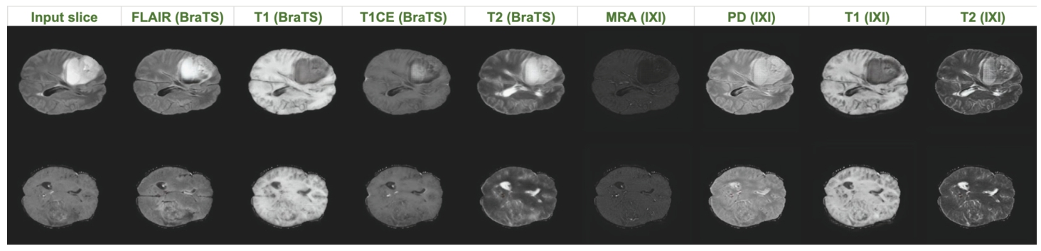
Fig. 2
‘Glomerular hemorrhage’ was detected in T2 (right) instead of T1 (left).

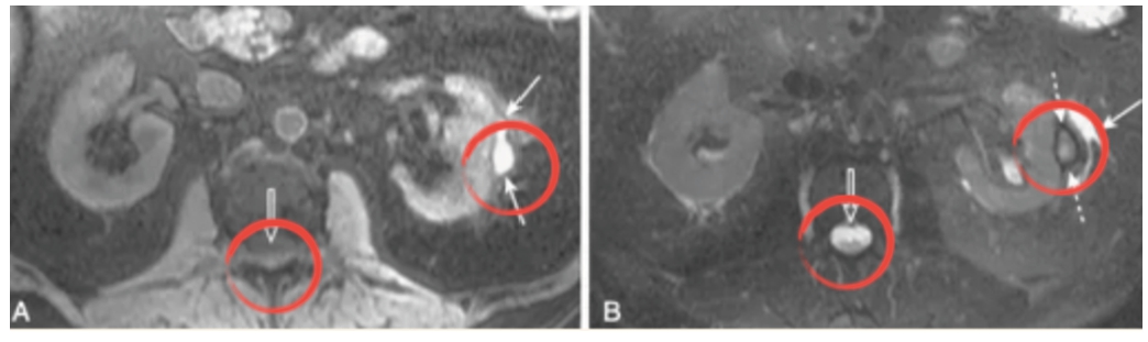
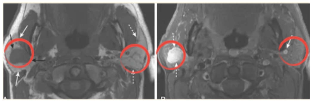
Fig. 3
‘Parotid pleomorphic adenoma’ detected in T1CE (right) instead of T1 (left).
3. Thirdly, both qualitative and quantitative results are generated on multicontrast MRI synthesis tasks using the ResUnet generator and StarGAN generators.

The aim of this research is to generate MRI images with diverse contrasts solely from a single MRI image. For instance, given an input MRI image acquired with a T1 pulse sequence, the model can generate MRI images with T2, MRA, FLAIR contrasts, and more (as depicted in Fig. 1). This innovative approach has the potential to yield substantial benefits, including cost savings, time efficiency, and reduced patient discomfort, by eliminating the necessity for multiple MRI scans that require patients to remain motionless for prolonged periods. Moreover, taking the same anatomical structure in a different pulse sequence can assist diagnosticians in detecting underlying pathologies or injuries, such as brain tumours or oedema, as illustrated in Figs. 2, 3, and 4.

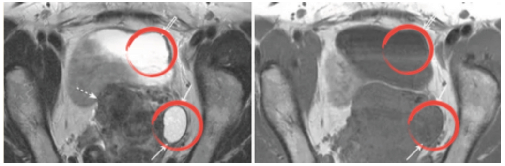
Fig. 4

‘Simple ovarian cyst’ detected in T2 (left) instead of T1 (right).

The remainder of this paper is structured as follows. Section 2 provides an overview of related work in MRI synthesis using deep learning. The methodology and architecture of the proposed GAN-based approach are described in Section 3. Then, the experimental setup and results are detailed in Section 4. Finally, Section 6 concludes the paper and discusses potential future directions for research in MRI synthesis using deep learning models.

2Related Works

2.1Medical Image-to-Image Transformation

Recent studies have examined the application of deep learning models for MRI synthesis, aiming to generate diverse MRI images with different contrasts. These approaches have leveraged various techniques and architectures to achieve accurate and realistic synthesis results. One prominent approach in MRI synthesis is the utilization of generative adversarial networks (GANs). Sohail et al. (2019) introduced a method for synthesizing multi-contrast MR images without paired training data. The proposed approach utilizes GANs to learn the mapping between input images and target contrasts. Adversarial and cycle-consistency losses are employed to ensure the generation of high-quality and realistic multi-contrast MR images. In another study, Zhu et al. (2017) suggested an approach that bears similarities to the method introduced in Sohail et al. (2019). However, this method utilizes cycle-consistent adversarial networks (CycleGAN) to learn mappings between only two different image domains. By employing two separate generator networks and two discriminator networks, the model performs both forward and backward translations between the domains. The cycle-consistency loss ensures that the reconstructed images from the translated images remain close to their original counterparts. Experimental results demonstrate the effectiveness of CycleGAN in various image translation tasks, including style transfer, object transfiguration, and season translation.

Wei et al. (2018) proposed a method to enhance the training of Wasserstein-GANs by introducing a consistency term. The consistency term ensures that the generated samples are consistent under small perturbations in the input noise space. This term helps stabilize the training process and improve the quality of generated samples. They also introduced the concept of the dual effect allowing the generator to capture more diverse modes of data distribution. Experimental results demonstrate that the proposed method outperforms the original WGAN and other state-of-the-art GAN variants in terms of image quality, diversity, and stability.

In recent advancements in medical imaging, several methods have emerged to enhance MRI image resolution such as Zhang et al. (2023) using Dual-ArbNet and Chen et al. (2023) with CANM-Net. Additionally, another study has been conducted to increase the resolution and remove noise from 2D images using Transformer GANs by Grigas et al. (2023). In general, although the task is named super-resolution, it can still be considered a sub-category of image synthesis. It can be observed that in recent years, GANs have played a crucial role and have been widely applied in tasks related to brain MRI images, especially with the majority of studies aiming at MRI image synthesis applications, according to statistics from Ali et al. (2022).

However, it can be seen that most of the above methods have limitations to provide single-input multi-output (SIMO) MRI image synthesis, which could be extremely beneficial, especially under circumstances where only a single modality is available but multiple contrasts are necessary for diagnosis and treatment planning. Moreover, it is imperative to develop an approach that facilitates training on multiple datasets to enhance the diversity of learning data and improve the synthesizing performance.

2.2Multi-Domain Image-to-Image Transformation

StarGANs represent one of the pioneering attempts to address multi-domain image-to-image translation within a single dataset (Nelson and Menon, 2022). This innovation allows the generator G to transform a single image X to an output image Y conditioned by the expected target domain c:G(X,c)→Y. To achieve this, the input image is combined with the target domain information to form the input for the generator (Choi et al., 2018).

By incorporating the target domain information during the synthesis process, StarGANs effectively enable the generator to adapt its output based on the specified domain. This conditioning mechanism facilitates the translation of images across various domains within a single training dataset, eliminating the need for separate models or training processes for each specific domain. The generator, equipped with the ability to utilize the target domain information, can effectively learn the mapping between the input image and the desired output in a domain-specific manner (Choi et al., 2020).

While StarGan has shown impressive results in multi-domain image-to-image translation, the original research did not explore its application in the medical domain. Furthermore, the original architecture simply consisted of a straightforward CNN with a few layers. As a result, several subsequent efforts have focused on modifying the architecture and adapting the StarGan approach to medical datasets. Building upon it, this study also aims to further enhance the method and prove its capacity in the medical domain.

3Methodology

The design methodology of this research is built upon a set of fundamental principles. Firstly, simplicity and generality are given utmost priority in the model architecture, while also ensuring its robustness to capture intricate features and facilitate efficient training. Secondly, emphasis is placed on leveraging information from various aspects during the optimization process to enhance the model’s generalization capabilities. This section entails how those principles converge to the proposed modification to the original design.

3.1Generator

3.1.1StarGANs-Based Generator Architecture

The first approach in this study is StarGANs, based on the architecture of CycleGAN, utilizing a generator network with two downsampling convolutional layers, six residual blocks, and two upsampling transposed convolutional layers. Instance Normalization is applied to the generator, while no normalization is used for the discriminator (Bharti et al., 2022). The detailed architecture is shown in Fig. 5.

Fig. 5

Illustration of the StarGANs generator architecture.

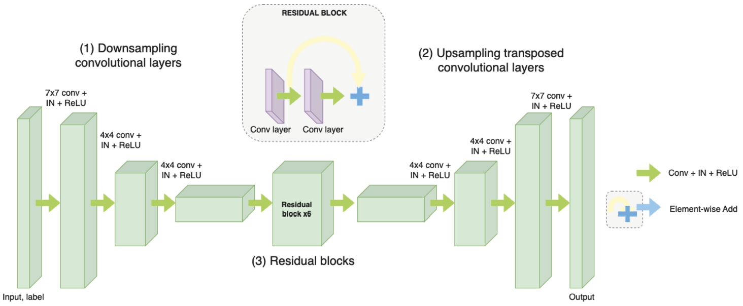
• Downsampling Convolutional Layers: The two downsampling convolutional layers are responsible for reducing the spatial dimensions of the input image (Hien et al., 2021). Convolutions are applied with a stride size of two, which effectively downsamples the image and captures the coarse features.
• Residual Blocks: These parts play a crucial role in capturing fine-grained details and enhancing the gradient flow through the network. Each residual block consists of two convolutional layers with batch normalization and ReLU activation functions. The residual connection allows the network to learn residual mappings, which helps in alleviating the vanishing gradient problem and enables the network to learn more complex representations.
• Upsampling Transposed Convolutional Layers: The two upsampling transposed convolutional layers perform the opposite operation of the downsampling layers. They increase the spatial dimensions of the features, allowing the generator to reconstruct the output image with higher resolution (Hien et al., 2020). These layers use transposed convolutions with a stride size of two, effectively upsampling the features.
• Instance Normalization: Instance normalization is applied to the generator. It normalizes the activations within each instance (sample) in the batch, making the network more robust to variations in instance statistics. By applying instance normalization, the generator can effectively capture and preserve the style and texture information of the input image during the translation process.

3.1.2ResUNet Architecture

It is observed that the shallow design of the standard architecture might struggle to capture fine-grained information at multiple scales. To address that concern, a ResUNet generator is utilized, which incorporates feature fusion at multiple scales for the image-to-image translation task. The ResUNet network is constructed by stacking multiple modified residual blocks (ResBlock) in an encoder-decoder fashion (U-Net). In line with the U-Net design, this approach also maintains a symmetric architecture, as depicted in Fig. 6. The ResUNet generator starts with 2 downsampling ResBlocks, followed by an encoder ResBlock, an upsampling ResBlock, and a final ResBlock called Decoder. The generation of the output is facilitated by a convolutional layer. The subsequent sections provide a detailed exploration of the architecture and its functionality:

Fig. 6

Illustration of the ResUNet architecture as a generator.

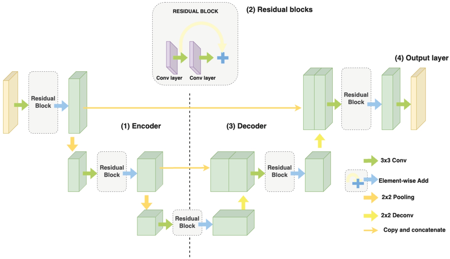
• Encoder: Positioned on the left side of the dashed line, the encoder consists of Downsampling Blocks, each composed of Residual Blocks. Within each Residual Block are two convolutional layers accompanied by batch normalization and ReLU activation functions. Notably, there’s an additional AvgPool layer at the conclusion of the Residual Block, tasked with diminishing the spatial dimensions of the input image.
• Decoder: The right-hand side of the dashed line consists of upsampling blocks. Similar to the Encoder, each upsampling block is composed of residual blocks; however, contrary to downsampling, at the end of each Residual Block, there is a deconvolution layer to upscale the generated image, along with skip connections from the Encoder. These skip connections fuse the high-resolution features from the encoder with the upsampled features, enabling the reconstruction of detailed and high-quality images.
• Output Layer: This is the final layer of the generator and typically employs a suitable activation function, such as sigmoid or tanh, to map the output values to the desired range. This layer generates the translated image in the target domain based on the learned features and the input image.

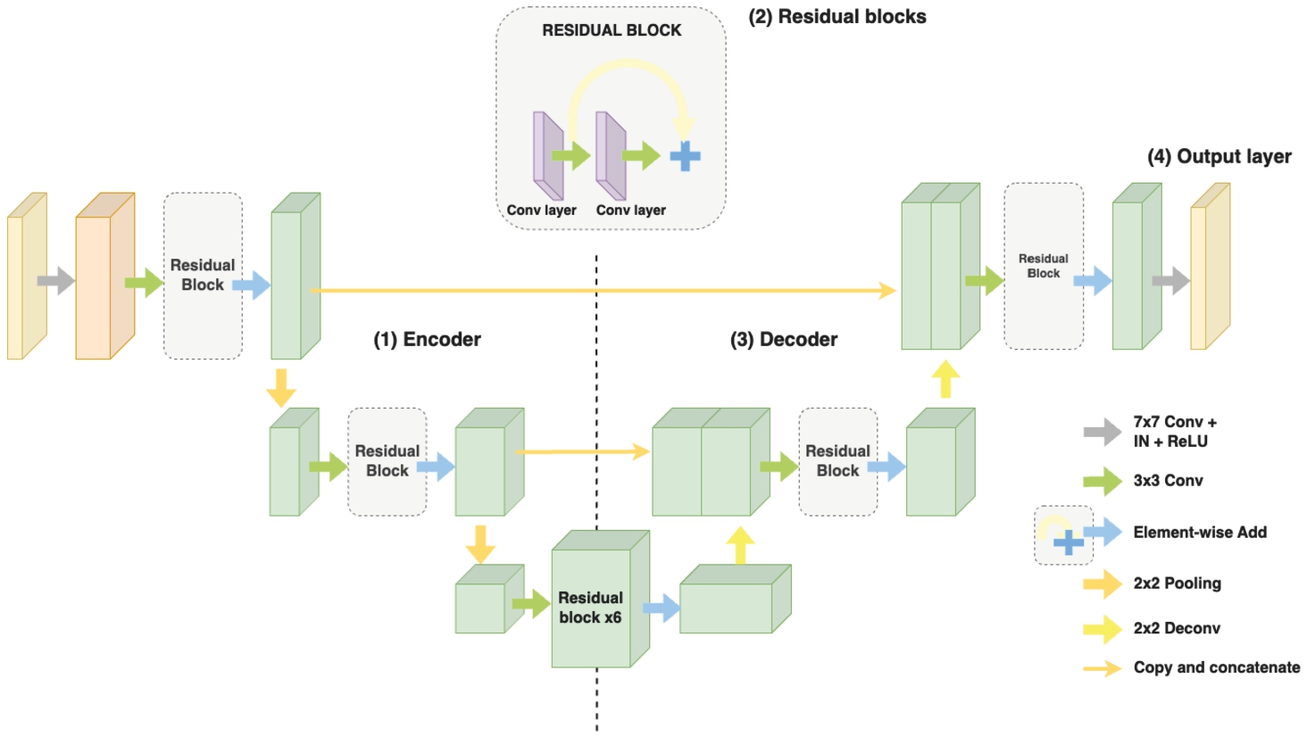
3.1.3Proposed Generator Architecture

After conducting experiments with the ResUNet architecture, a drawback was observed, which is that the generated MRI images, although exhibiting relatively good structural features, do not accurately represent the colours and components of the brain. It is speculated that the extensive use of Residual Blocks throughout the network and concatenation of all the encoder outputs to the decoder input causes the model to learn excessive colour features from the source image and introduce colour discrepancies in the generated images. Meanwhile, images generated by StarGANs exhibit high colour accuracy, addressing the shortcomings of ResUNet, yet face challenges in ensuring fine-grained details and high resolution.

Therefore, the image generation capability of the StarGANs network and the feature extraction capability of the ResUnet network will be leveraged in this research. Specifically, the main components of the ResUnet network, including ResBlock, Encoder, and Decoder, are retained. Additionally, two 7×7 convolutional layers are added followed by instance normalization layers and a ReLU activation function at the two ends of the network (Hien et al., 2021). This research aims to reduce the gradient of the network and allow the model to retain features while still flexibly generating images, ensuring that the colours of the generated images differ from the input images (e.g. image T1 has contrasting colours with image T2). Therefore, the resblock block in the bottleneck section is replaced with 6 Residual Blocks, adapting from Choi et al. (2018). This modification aims to make the network less deep and reduce the dominance of dense concatenation, which may have been contributing to the colour discrepancies. The detailed architecture summary is described in the Appendix section, in Table 6.

Fig. 7

Illustration of the proposed generator architecture.

3.2Discriminator

The discriminator is responsible for classifying whether an input image is real or fake, and also predicting the class label of the image in the case of conditional GANs. It follows the PatchGAN architecture (Choi et al., 2018; Zhu et al., 2017), which operates on local image patches rather than the whole image.

Fig. 8

Illustration of the discriminator architecture.

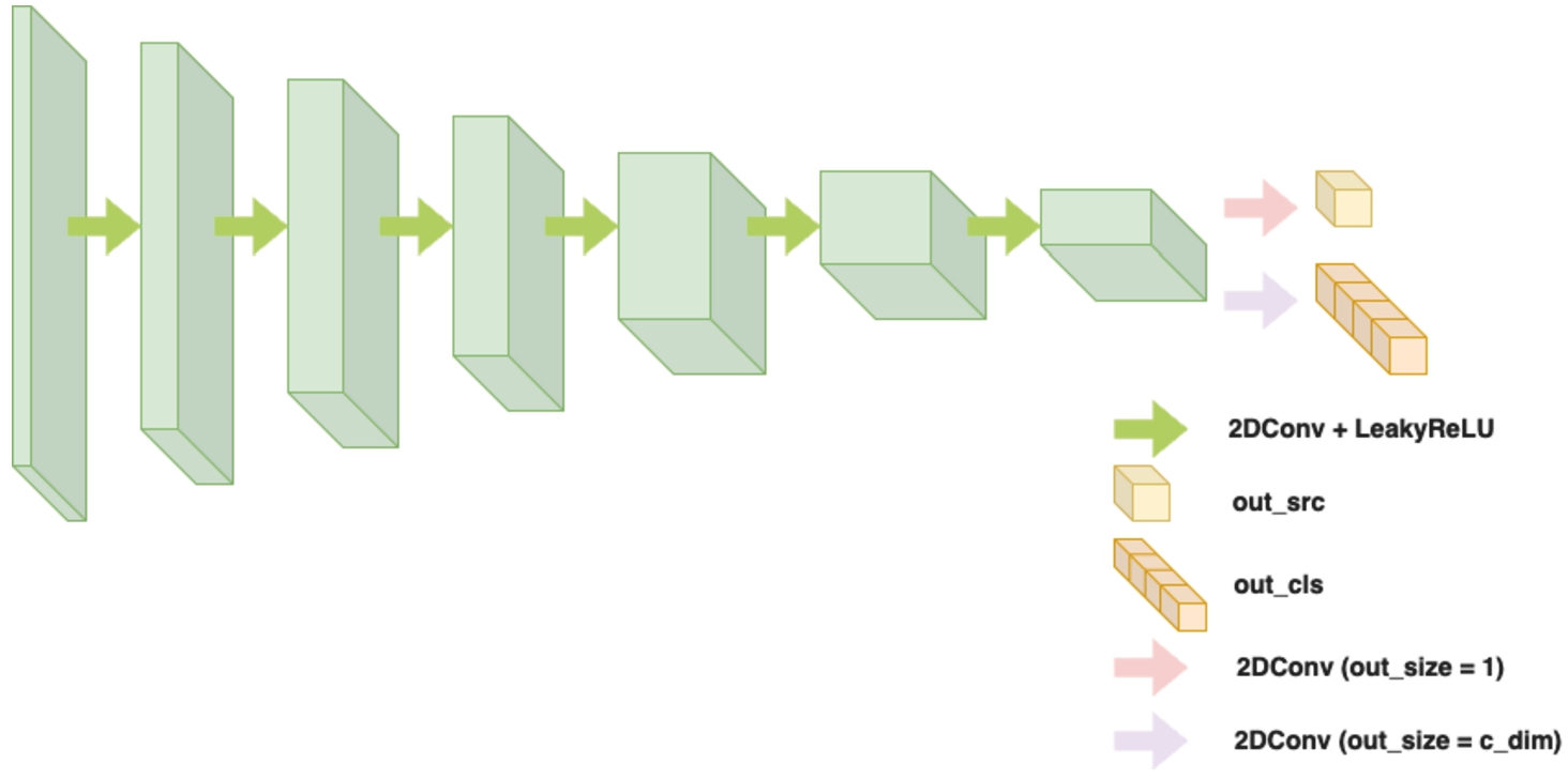
The main part of the discriminator contains the stacked convolutional layers, accumulating the number of channels to capture more complex features. The output of these layers is then passed through two separate convolutional layers, as shown in Fig. 7 and Fig. 8.

The structure of the Discriminator in StarGAN is similar to a typical Discriminator, but it includes two separate convolutional layers near the final layer to generate two distinct outputs: the first output represents the probability of the image being real or fake, while the second predicts the class label. The discriminator is designed to handle images of varying sizes, and its architecture promotes the learning of local image details for accurate discrimination. The detailed architecture summary is described at Table 7.

3.3Loss Functions

The main purpose of GANs in general and this study approach, in particular, is to make the generated images indistinguishable from real images, an adversarial loss of typical GANs (Bharti et al., 2022) is adopted, defined

(1)

Ladv=Ex[logDsrc(x)]+Ex,c[log(1−Dsrc(G(x,c)))],

where G creates an image G(x,c) based on both the input image x and the specified target domain label c, while D aims to differentiate between real and generated images. Throughout this paper, the probability distribution over sources provided by D is denoted as Dsrc. The primary aim of the generator G is to minimize this objective, while the discriminator D aims to maximize it.

3.3.1Multi-Domain Image-to-Image Translation

Adversarial loss: Instead of utilizing the adversarial loss in typical GANs (Eq. (1)), which has been observed to encounter challenges such as mode collapse, vanishing gradients, and hyper-parameter sensitivity, he regularized Wasserstein GAN with gradient penalty WGAN-GP is employed. This choice ensures stable training for both the generator and discriminator networks while also improving the overall image quality of the generated outputs. The WGAN-GP loss function is defined as follows:

(2)

Ladv=LWGANgp+λctCT|x′,x″.

In the above formulation, the initial term represents the WGAN-GP loss, while the second term introduces a consistency term to regularize this loss. The WGAN-GP loss is expressed as follows:

(3)

LWGANgp=E[Dsrc(x)]+Ex,c[Dsrc(G(x,c))]−λgpExˆ[(‖∇xˆDsrc(xˆ)‖2−1)2],

where xˆ is sampled uniformly along a straight line between a pair of real and generated images. Specifically, Gulrajani et al. (2017) presented a gradient penalty approach, highlighting that a differentiable discriminator Dsrc maintains 1-Lipschitz continuity when the norm of its gradients remains at or below 1 universally.

(4)

CT|x′,x″=Ex∼P[max(0,d(D(x′),D(x″))+0.1·d(D_(x′),D_(x″)−M′)].

In particular, x′ and x″ represent virtual data points that are in proximity to x. D(x′) represents the discriminator’s output when provided with input x, while D_ refers to the output of the second-to-last layer discriminator. And d represents the distance between two data points. M′ in the above formula is a constant by which d is bounded as assumed by Wei et al. (2018)

Contrast classification loss: In order to achieve the desired image translation, an auxiliary classifier is introduced on top of the discriminator D. This involves optimizing D using a domain classification loss for real images and optimizing G using a domain classification loss for fake images. The following are defined for real images:

(5)

Lclsr=Ex,c′[−logDcls(c′|x)],

where the expression Dcls(c′|x) denotes a probability distribution over domain labels determined by D. Through minimizing this objective, D is trained to classify a real image x to its original domain c′. It is assumed that the training data provides the input image and its associated domain label pair (x,c′). On the flip side, the below formula is the loss function for distinguishing fake images within the domain:

(6)

Lclsf=Ex,c′[−logDcls(c′|G(x,c))].

In particular, x and c′ represent a real image and its original label, respectively. G(x,c) and c denote a generated (fake) image and the desired target contrast.

For this experiment, Softmax Cross Entropy is utilized to compute the classification loss.

Cycle consistency loss: To enforce a reliable one-to-one mapping between the source and target image domains, a cycle consistency loss is utilized in the compound loss. This loss term ensures that the generated images can faithfully reconstruct the original source image when translated back to the source domain. By incorporating the cycle consistency loss, the model becomes more robust and capable of producing consistent and accurate image translations. In this experiment, L1-norm is applied to compute cycle consistency loss:

(7)

Lcyc=Ex,c,c′[‖x−G(G(x,c),c′)‖].

3.3.2New Generation Loss Functions with DSSIM and LPIPS

For the generator, the L1-norm has already been applied for cycle-consistent loss, but the current L1 loss disregards patch-level dissimilarity among images, limiting the information available for the generator. To overcome this limitation, two additional terms are introduced in the generation loss, promoting small-scale dissimilarity between real and reconstructed images at the patch level. This enhances the generator’s available information.

Motivated by the effectiveness of measuring structural similarity between images using the Structural Similarity (SSIM) metric in a patch-wise manner, the Structural Dissimilarity Loss (DSSIM) is adopted as an extension of SSIM:

(8)

LDSSIM=Ex,c,c′[(1−SSIM(x−G(G(x,c),c′)))2].

In particular, SSIM is formulated as:

(9)

SSIM(x,y)=(2μxμy+C1)+(2σxy+C2)(μx2+μy2+C1)(σx2+σy2+C2),

with:

μx, μy: the pixel sample mean of x and y, respectively;

σx2, σy2: the variance of x and y, respectively;

σxy: the covariance of x and y;

C1=(k1L)2, C2=(k2L)2: two variables to stabilize the division with weak denominator;

L: the dynamic range of the pixel-values (typically this is 2#bits per pixel−1);

k1=0.01 and k2=0.03 by default.

Additionally, to ensure that the generator continuously generates images that closely match the target contrast, the Learned Perceptual Image Patch Similarity (LPIPS) metric is incorporated, which has been recently proposed:

(10)

LLPIPS=Ex,c,c′[x−G(G(x,c),c)].

The ultimate reconstruction loss combines the desirable aspects of all three terms:

(11)

Lrec=λcycLcyc+λDSSIMLDSSIM+λLPIPSLLPIPS.

3.3.3Full Objective

In summary, the proposed loss function for the generator and discriminator networks can be formulated as follows:

(12)

LD=−Ladv+Lclsr,

(13)

LG=Ladv+λclsLclsf+λrecLrec.

4Experimental Results

4.1Dataset Detail and Data Preprocessing

To evaluate the method, 2 standard medical image datasets, namely BraTS2020 and IXI, are adopted in this study.

4.1.1Dataset Detail

BraTS2020: The BraTS2020 dataset is a widely used benchmark dataset for brain tumor segmentation in magnetic resonance imaging (MRI). It consists of multi-modal MRI scans, including T1-weighted, T1-weighted contrast-enhanced, T2-weighted, and Fluid Attenuated Inversion Recovery (FLAIR) images (indicated in Table 1).

IXI dataset: The IXI (Information eXtraction from Images) dataset is a comprehensive and publicly available collection of multimodal brain imaging data. 600 MR images from normal, healthy subjects are collected with 4 acquisition protocols: T1-weighted, T2-weighted, Proton Density (PD), and Magnetic Resonance Angiography (MRA) (indicated in Table 2).

Table 1

Detailed information on the BraTS2020 dataset.

Attributes	Detailed information
Number of contrasts	4 (T1, T2, T1CE, FLAIR)
Number of samples per contrast	494 images/contrast
Image size (3D image)	Already registered
	All images: (240×240×155)
Ratio healthy/disease (tumour)	40/60

Table 2

Detailed information on the IXI dataset.

Attributes	Detailed information
Number of contrasts	4 (T1, T2, PD, MRA)
Number of samples per contrast	568 images/contrast
Image size (3D image)	Not registered:
	T1: (256×256×150)
	T2: (256×256×130)
	MRA: (512×512×100)
	PD: (256×256×130)
Ratio healthy/disease (tumour)	100/0

4.1.2Data Preprocessing

For both datasets, the nibabel library is employed to manage the loading and saving of MRI image files in .nii format.

BraTS2020: Since all of the images had already been registered to the same template with size (240, 240, 155), there is no need to apply any registering method for this dataset. The middle axial slices of 4 contrasts are shown in Fig. 9.

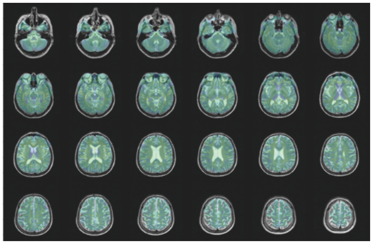
Fig. 9

Illustration of axial slices of the BraTS2020 dataset.

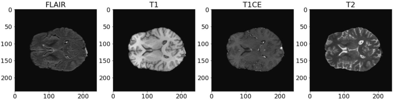
The original BraTS2020 dataset has already been divided into a training set and a validation set, as presented in Table 3. Since the images of the BraTS2020 dataset provide better resolution in the axial plane, axial slices of all images were taken. For this experiment, 10 slices per 3D image are taken.

IXI dataset: Upon reviewing and analysing the entire IXI dataset, it was observed that there are 2 contrasts that exist in different templates from the remaining. The middle original slices of the 4 contrasts are shown in Fig. 10:

Table 3

Number of samples per contrast in the BraTS2020 dataset.

Train	FLAIR	3690
	T1	3690
	T1CE	3690
	T2	3690

Test	FLAIR	1250
	T1	1250
	T1CE	1250
	T2	1250

Fig. 10

Illustration of axial slices of IXI dataset before registration.

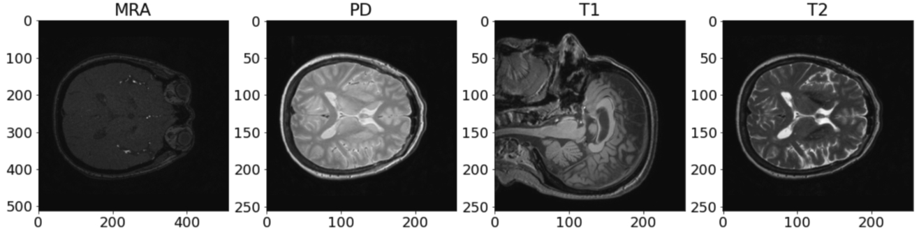
As depicted in Fig. 10, it is evident that MRA images are in shapes (512, 512, 100), while T1 images are in completely different templates (size and plane). However, it is noteworthy that there are still PD and T2 images in the same template and similar to BraTS2020 images. In light of this observation, the decision is made to apply some registering transformations to MRA and T1 images using the common template synthesized from PD and T2. For this experiment, an affine transformation is employed from the AntsPy package (Avants et al., 2009) which is a Python library that wraps the C++ biomedical image processing library ANTs. First, a common template is extracted from two classes: PD and T2. Subsequently, a mask is derived from this template and subsequently the T1 and MRA images are registered onto the mask using affine transformation, as mentioned in Sohail et al. (2019). The preprocessing process for the IXI dataset is depicted in Figs. 11, 12, and 13.

Fig. 11

The axial slices of a common template synthesized from PD and T2 images.

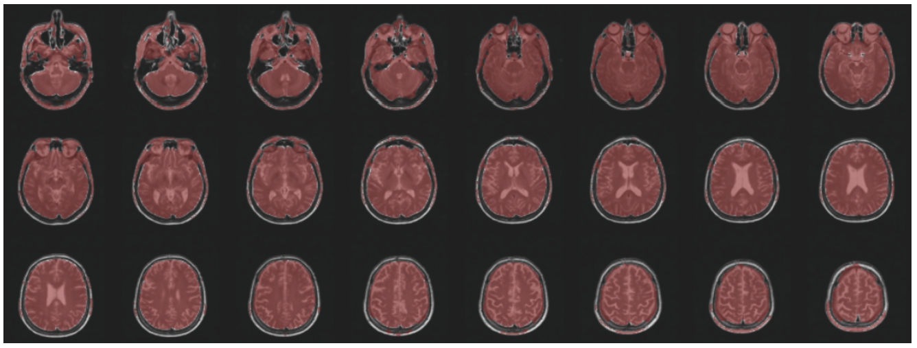
Fig. 12

The axial slices of MRA/T1 when embedded in the common template.

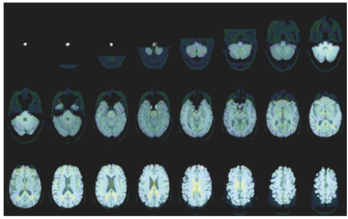
Fig. 13

The axial slices of MRA/T1 after applied affine transformation.

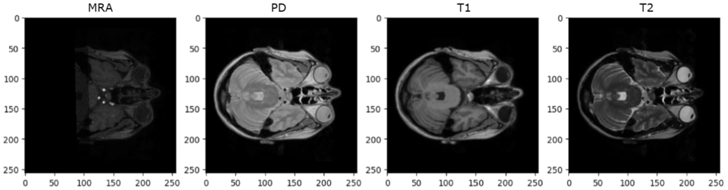
This provides 568 images of the same size and position from which 68 were randomly selected for testing while the remaining 500 were used for training. Since the MRA images of the IXI dataset provide better resolution in the axial plane, axial slices of all images were taken (as shown in Fig. 14). For the IXI dataset, only 5 middle slices per 3D image are selected. This decision is made due to the presence of missing or noisy images in some contrasts (as shown in Figs. 15 and 16), particularly in MRA, when attempting to take 8 or 10 slices.

Fig. 14

Illustration of axial slices of IXI dataset after registration.

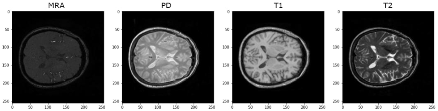
Fig. 15

Missing images in MRA contrast.

For data preprocessing, transformations including horizontal flipping, resizing to 256×256, and normalization are applied. Table 4 and Fig. 17 indicate the number of samples in the IXI dataset and visualization of the distribution of actual collected data from both datasets.

Fig. 16

Blur images in MRA contrast.

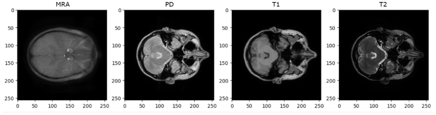
Table 4

Number of samples per contrast in the IXI dataset.

Train	MRA	2430
	PD	2430
	T1	2430
	T2	2430

Test	MRA	335
	PD	335
	T1	335
	T2	335

Fig. 17

Distribution of data from both datasets divided by datasets (BraTS2020/IXI).

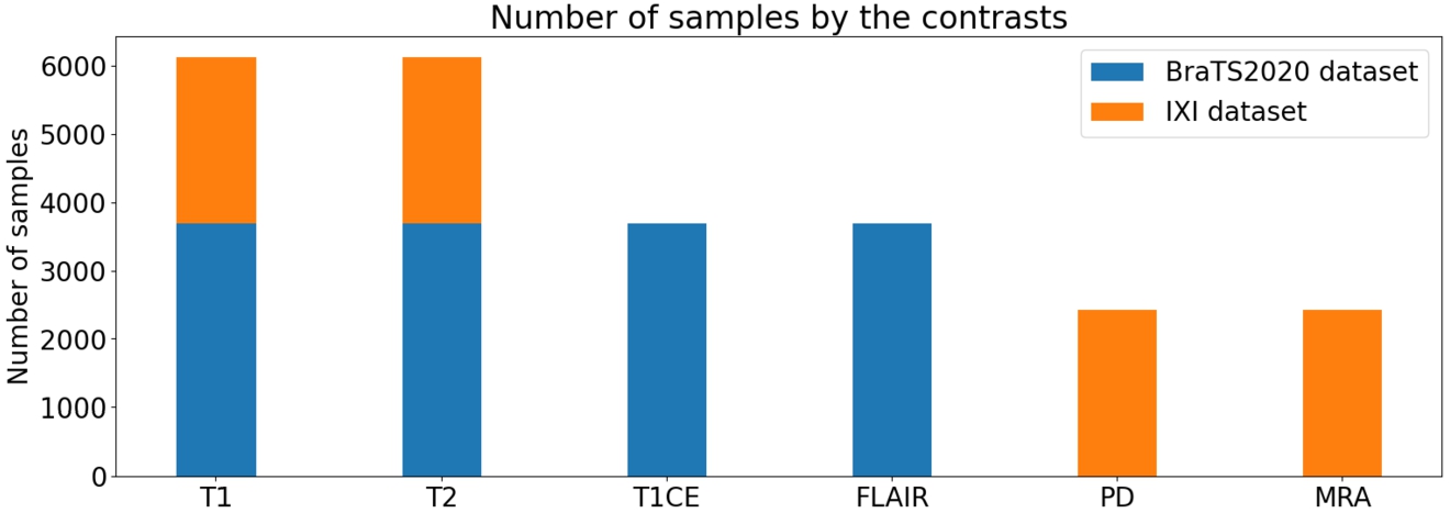
Fig. 18

Distribution of data from both datasets divided by brain’s condition (healthy/diseases).

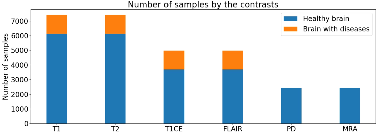
Regarding the number of samples per contrast, as depicted in Fig. 17, a notable imbalance is observed, with a higher number of samples in T1 and T2 compared to the other contrasts. However, this disparity falls within an acceptable range. In Fig. 18, there is a significant disparity in the number of samples between the two brain conditions (healthy/diseased). However, as the main purpose of this experiment is to focus on synthesizing MRI in general, this problem would be resolved in future approaches.

In Fig. 18, a substantial disparity in the number of samples between the two brain conditions (healthy/diseased) is evident. Nonetheless, it is important to note that the primary objective of this experiment is to focus on synthesizing MRI in general. The issue of sample disparity will be acknowledged and addressed in future approaches.

4.2Experimental Results

4.2.1Implementation Details

All experiments were conducted using the PyTorch framework. To accommodate computational limitations, the image slices were resized to dimensions of 256×256. During training, the input images and target contrast were randomly selected in an unpaired manner to ensure fairness in comparison (Xiang et al., 2018). Both the default StarGAN model and the proposed models used the same set of hyperparameter values. The training was carried out for 200,000 iterations with a batch size of 4. Through numerous hands-on trials, this study observed that the loss began to rise when the iteration count was configured to exceed 200,000. Furthermore, due to hardware constraints, the batch size could only be set to a value below 4 to prevent training process crashes. All models are trained using Adam optimizer with β1=0.5 and β2=0.999, as experienced by Kingma and Ba (2014). All models are trained with a learning rate of 0.0001 for the initial 100,000 iterations, followed by a linear decay of the learning rate to 0 over the next 100,000 iterations. In this study, adjustments were made to the learning rate, resulting in a marginal fluctuation of the loss value, which proved challenging to converge. The training process takes about one day when conducted on a single NVIDIA RTX-3060 GPU.

During the training process, the following parameters are employed: where λct and λgp are hyper-parameters that control the relative importance of consistent regularization and gradient penalty, respectively. Within it, consistent regularization plays a supportive role in complementing and improving the gradient penalty. Specifically, λct=1 (Eq. (2)) and λgp=10 (Eq. (3)) were selected after experimenting with neighbouring value ranges. In the training of this image generator, prioritization is given to image quality over classification. The reason is that image classification is relatively straightforward and dependent on the task of synthesizing images; the closer the generated images are to the ground truth, the higher the accuracy of the classification task will be. Additionally, image reconstruction is as important as image generation, leading to the setting of λcls=1 (Eq. (13)) and λrec=1 (Eq. (13)). As stated previously, when M′ varies within the range of 0 to 0.3, the experiments yield similar outcomes. Consequently, M′=0 (Eq. (4)) and λcyc=λDSSIM=λLPIPS=10 (Eq. (11)) are set uniformly across all experiments.

4.2.2Mask Vector for Training on Multiple Datasets

The aim of this experiment is to integrate multiple datasets during model training to mitigate the limitations posed by data scarcity in medical image synthesis. However, a challenge arises when incorporating multiple datasets, as each dataset only holds partial knowledge regarding the label information.

In the specific scenario of using datasets like BraTS2020 and IXI, a limitation arises where one dataset (BraTS2020) includes labels for contrasts: T1, T2, T1CE, and FLAIR but lacks labels for other contrasts such as PD and MRA, while the other dataset (IXI) is the opposite (lack of T1CE and FLAIR). This poses a challenge because the reconstruction of the input image x from the translated image G(x,c) requires complete information on the label vector c′.

To address this issue, a mask vector is adopted, denoted as m, which was introduced in the StarGAN framework. The purpose of the mask vector is to allow the model to ignore unspecified labels and focus only on the explicitly known label provided by a particular dataset. In the context of the paper, m is an n-dimensional one-hot vector, where n is the number of datasets. Each element of the mask vector indicates whether the corresponding dataset label is specified or not.

(14)

c_=[c1,…,cn,m]

For example, if n=2 as mentioned in the paper (representing two datasets, BraTS2020 and IXI), and if a sample belongs to the BraTS2020 dataset, then the mask vector m can be represented as [1,0], indicating that the first dataset label (BraTS2020) is specified while the second dataset label (IXI) is unspecified. This approach helps the model to handle multiple datasets efficiently, focusing on relevant labels while ignoring irrelevant ones.

In the defined expression, [·] denotes concatenation, and represents a vector containing the labels for the ith dataset. The vector, which represents the known labels, can take the form of a binary vector for binary attributes or a one-hot vector for categorical attributes. The remaining n−1 unknown labels are assigned zero values. In the specific experiments conducted, the BraTS2020 and IXI datasets are utilized, resulting in a value of n equal to two.

4.2.3Qualitative Evaluation

Fig. 19

Synthesis of MRA, PD-weighted and T1-weighted images using a single T2-weighted image as input (IXI dataset).

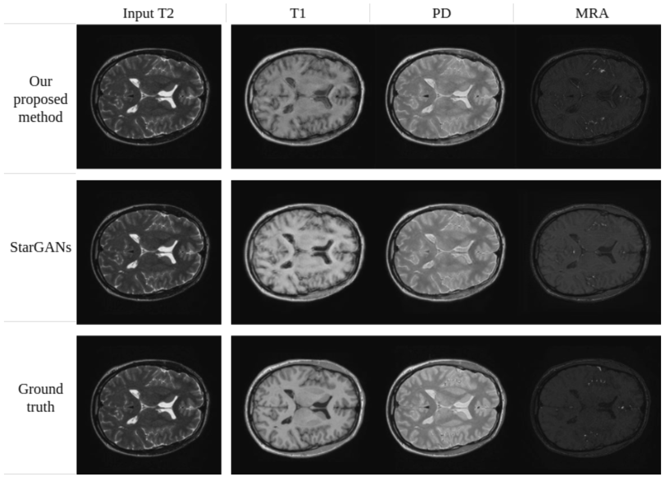
Fig. 20

Synthesis of T1-weighted, T2-weighted, and FLAIR images using a single T1CE-weighted image as input (BraTS2020 dataset).

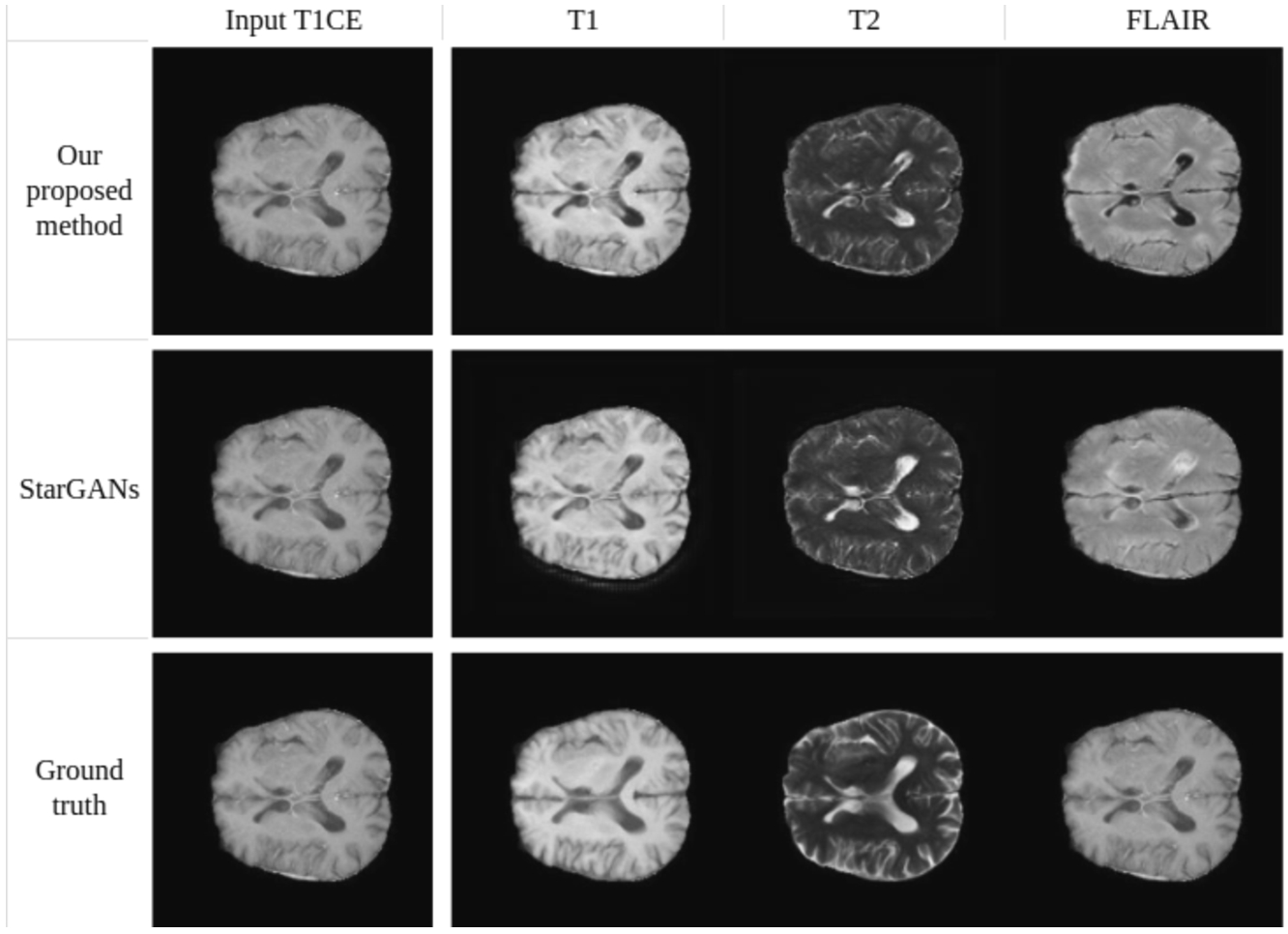
Figures 19 and 20 provide a qualitative comparison between the proposed method and Star-GAN in terms of multi-contrast synthesis. The results demonstrate that Star-GAN partly fails to capture structural and perceptual similarities for small anatomical regions, which are effectively captured by the proposed method. In Fig. 19, the synthesis of MRA from a T2-weighted image shows that Star-GAN struggles to reproduce the accurate colour of the image, while the proposed method successfully generates an image that is nearly identical to the real one. Similarly, Fig. 20 with FLAIR contrast.

4.2.4Quantitative Evaluation

In order to evaluate the performance of the proposed model trained on multiple datasets compared to Star-GAN and the training experiment conducted on a single dataset, well-established metrics such as peak signal-to-noise ratio (PSNR), structural similarity index (SSIM) [21], and normalized mean absolute error (NMAE) are utilized [22]. The average results on BraTS2020 and IXI datasets are presented in Table 5. A higher PSNR and SSIM, as well as a lower NMAE, indicate better quality in the generated images. The experimental evaluation encompasses StarGANs (SG), ResUNet (RU), and the proposed methods: With two training strategies (training on a single dataset and multiple datasets); With new generation losses and new generator architecture. The proposed approach has acquired better performance than that of Star-GAN in evaluating PSNR and NMAE, demonstrating superior performance.

Table 5

Quantitative results.

	Metric	SG single¹	RU single²	SG both³	RU both⁴	Proposed method^∗
BraTS2020	SSIM	0.8166	0.7672	0.8238	0.7734	0.8167
	PSNR	34.578	35.959	34.632	35.327	35.847
	NMAE	0.0426	0.0412	0.0431	0.0427	0.0414
IXI	SSIM	0.6883	0.6854	0.7310	0.6913	0.6972
	PSNR	38.289	40.214	40.469	40.848	40.882
	NMAE	0.0437	0.0399	0.0392	0.0387	0.0384

¹StarGANs model trained on 1 dataset.

²Model with ResUnet generator trained on 1 dataset.

³StarGANs model trained on multiple datasets.

⁴Model with ResUnet generator trained on multiple datasets.

Regarding the comparison of architecture between the two models, it is observed that the StarGANs-based with ResUNet (RU) and proposed generator outperformed default StarGANs (SG) in most of the metric values, particularly in terms of metrics PSNR and NMAE, for both training strategies. Table 5 reveals that model RU single yields the best results in 2 metrics on the BraTS2020 dataset with PSNR = 35.959 and NMAE = 0.0412, followed by the second-best performance from the proposed model. However, because RU single is trained solely on the BraTS2020 dataset, which contains both healthy normal brain MRI images and brains with tumours or abnormalities, instead of being trained on both BraTS2020 and IXI datasets, it’s plausible that it may achieve superior performance compared to a model trained on both datasets. This is because the IXI dataset only consists of healthy normal brain MRI images. Upon close examination, the difference between the top-performing outcome and the second-best outcome is minimal. Additionally, the proposed model exhibited the best performance across all three metrics on the IXI dataset. This underscores the model’s robustness and its capability to adapt effectively when trained on diverse datasets.

On the other hand, when comparing the metrics between training on a single dataset and training on multiple datasets on the same generator architecture, results show that training on multiple datasets yielded comparable or sometimes even better results compared to training on individual datasets. This approach can be applied to reduce time and computational costs without compromising the model’s performance (results in Table 5). After applying the proposed generator architecture, new generation losses, and training on both datasets. The results (*) are shown in the last column in Table 5. demonstrate superior effectiveness compared to previous methods, as indicated by higher SSIM and PSNR values and lower NMAE.

4.3Experience in Training

Throughout the training process, a rapid decrease in classification loss was observed, particularly within the first 1000 iterations for both datasets. However, with the IXI dataset, the classification loss remained stable at a value of zero. By contrast, for the BraTS2020 dataset, the classification loss occasionally fluctuated away from zero. This can be understood as the MRI images in the BraTS2020 dataset having similar colour characteristics, making it challenging for the model to learn these specific features and smaller details such as tumours and subtle brain oedema. On the other hand, the IXI dataset consists of healthy, normal brain images with relatively different colour characteristics between contrasts, providing more distinguishable features for the model to learn.

5Demonstration

A website has been developed as a platform to showcase the conducted experiments. This website serves as a repository of the research findings and provides a convenient means for accessing the experimental data, results, and related materials. The repository can be accessed via https://github.com/hanahh080601/Generate-MRI-FastAP. As illustrated in Fig. 21, the website offers a user-friendly interface, allowing visitors to navigate through the MRI Synthesis experiments, explore the data, and gain insights into the research process. It serves as a valuable resource for researchers, practitioners, and interested individuals to access and review the experimental work conducted in this study.

Fig. 21

Illustration of the user interface for the demo website.

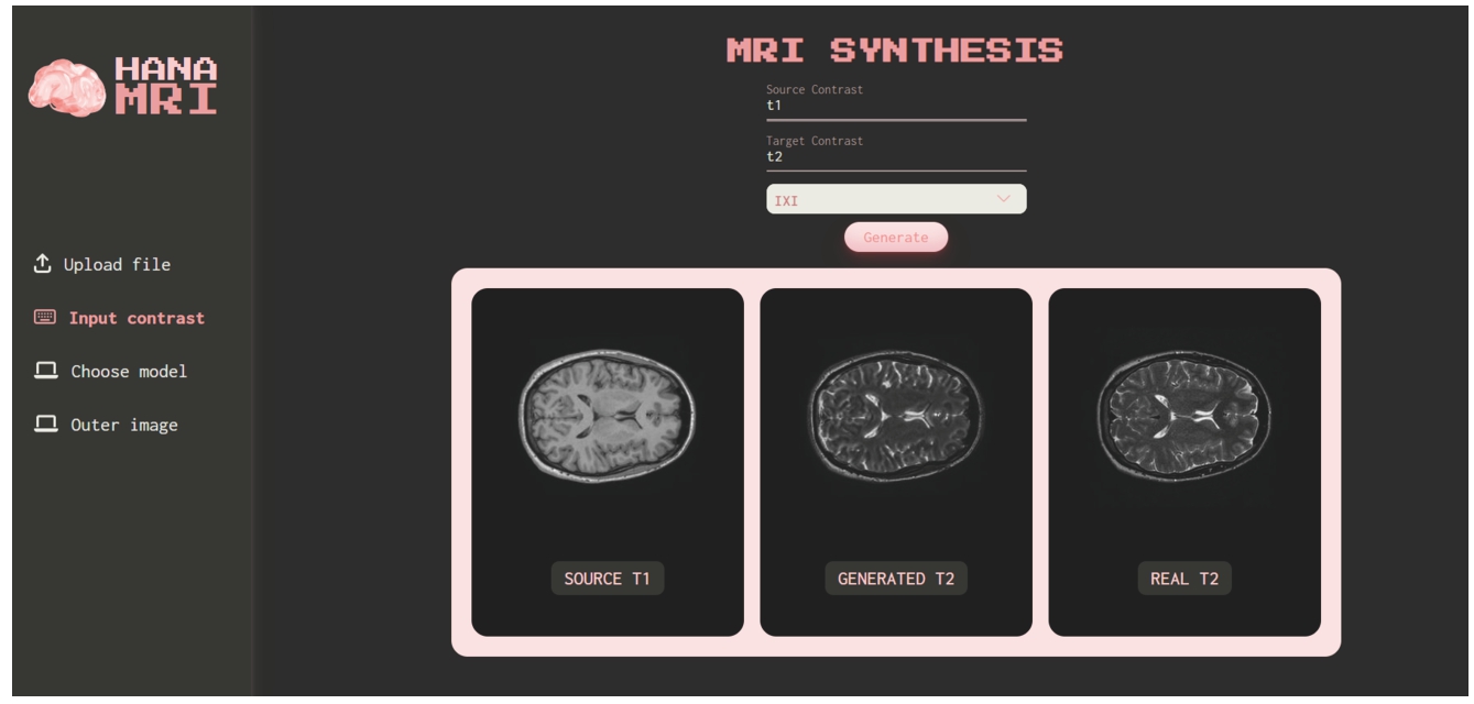
Specifically, users can select the input contrast and output contrast they desire for image synthesis upon accessing the website. They can then choose to upload files from their local device (the uploaded image must match the selected input contrast). Alternatively, users may only select the input and output contrast, after which the system will generate image using input data from the BraTS2020 and IXI datasets. This feature is used to qualitatively assess the quality of the generated images compared to the original ones.

Based on observation in Fig. 21, T1 is selected as the input contrast, T2 as the output contrast, and the IXI dataset is the chosen dataset. The system automatically chose a random T1 image from the test set of the IXI dataset and sent a request for the model to generate the T2 image. Additionally, the system also selected the ground truth T2 image from the dataset and displayed both for user comparison.

Fig. 22

Illustration of the testing model with low-resolution input image.

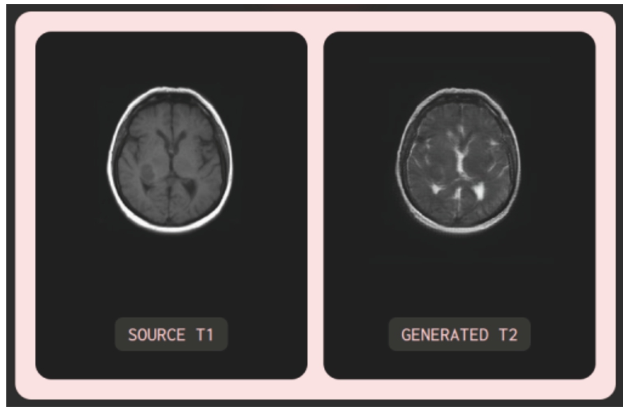
Fig. 23

Illustration of the testing model with input image T2 exhibiting abnormal fluid with the same colour as cerebral spinal fluid.

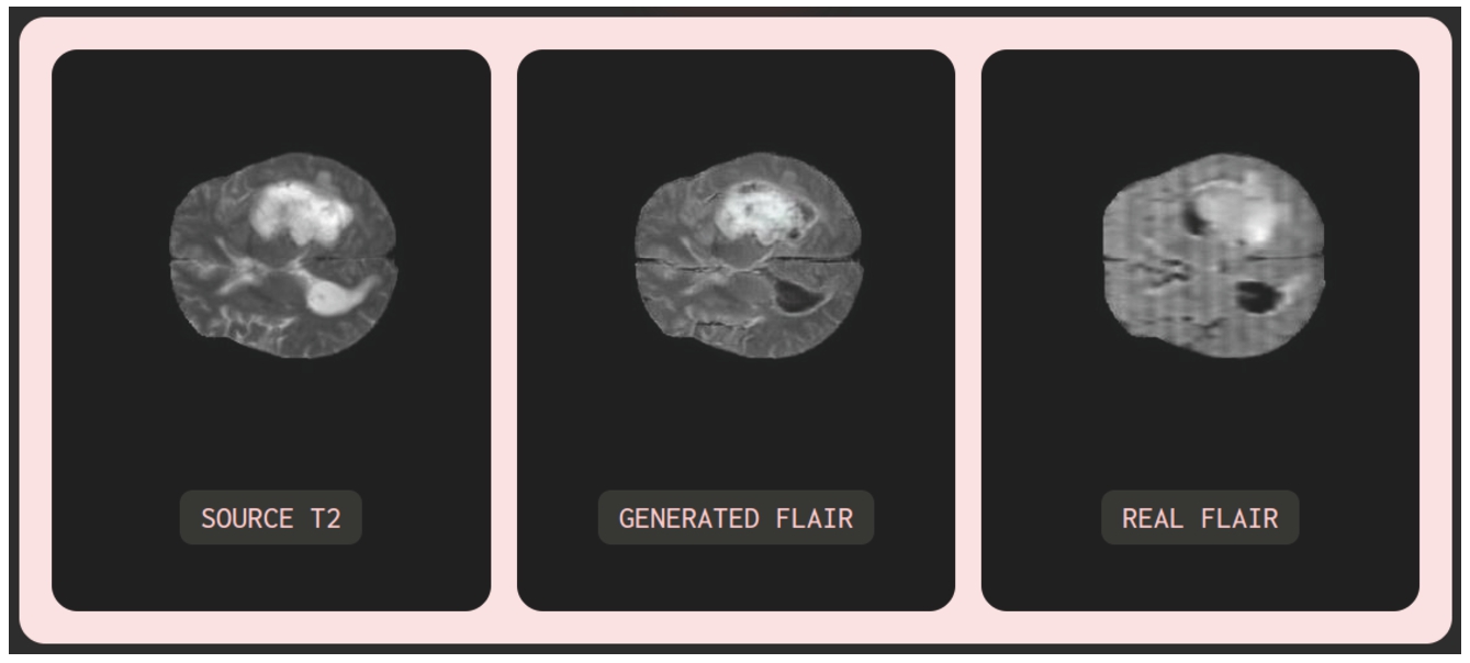
Moreover, testing was carried out to assess the model’s performance when presented with noisy or partially noisy input images. The experimentation was carried out on MRI images from the test datasets (BraTS2020 and IXI), as well as random images sourced from the Internet. Notable cases include input images corrupted with noise and T2 input images exhibiting abnormal fluid with the same colour as cerebral spinal fluid. Observing Fig. 22 with an input image of a noisy, low-resolution MRI T1 randomly obtained from the Internet, it can be seen that the generated image maintains the same quality (low resolution) as the input image, ensuring accuracy in colour contrast: cerebral spinal fluid, appearing dark in T1, manifests as bright in T2. In Fig. 23, with an input MRI T2 image from the BraTS2020 test dataset, the synthesized MRI FLAIR image exhibits relatively high image quality similar to the input image. Particularly, the model can learn and distinguish between cerebral spinal fluid (dark) and abnormal fluid (bright) in the generated FLAIR image while both appear bright in the T2 image. Furthermore, in reality, MRI images scanned by MRI machines may suffer from poor quality, noise, or misalignment due to objective and subjective factors, as illustrated by the REAL FLAIR image in Fig. 23. In such cases, the model-generated images rely solely on the input image without consideration of the MRI scanning process or subjective factors from the patient.

Therefore, this system can be utilized to synthesize multiple MRI images across various contrasts from just a single MRI image. This application can assist medical imaging specialists or diagnosing physicians by providing additional references in cases where they are uncertain about the original MRI image or desire to observe additional anatomical structures in a different contrast without requiring the patient to undergo additional MRI scans. This could help minimize costs, time, and partly support in making diagnoses.

6Conclustion

In this research, a novel method is proposed based on StarGANs, utilizing a ResUNet generator and a novel generation loss, for synthesizing multi-contrast MRI images. Despite substantial efforts made in prior studies (Bharti et al., 2022; Dai et al., 2020; Shen et al., 2020), the proposed approach only requires a single generator and discriminator. The results showcase that both qualitative and quantitative demonstrate the superiority of the proposed method over the default Star-GAN. Moreover, this study method overcomes the limitation of training multiple networks for multi-contrast image synthesis, which is crucial for deep learning methods reliant on multi-contrast data during training. The synthesized images produced by this method possess significant potential as highly valuable assets for medical professionals involved in research, education, and clinical applications.

Future work gears towards expanding the experiments to larger datasets in size and the number of contrasts, avoiding disparity in the proportion of healthy and diseased brain images. Additionally, efforts will be directed toward training the proposed approach with larger batch sizes and developing it into 3D images, which can significantly contribute to medical diagnosis in practical applications.

Appendices

A

ANetwork Architecture Details

Table 6

Proposed generator architecture summary.

Layer	Type	Details
Input	Conv2d	(13, 64, kernel_size=(7, 7), stride=(1, 1), padding=(3, 3), bias=False)
	InstanceNorm2d	(64, eps=1e-05, momentum=0.1, affine=True, track_running_stats=True)
	ReLU	(inplace=True)
down_block1	Conv2d	(64, 128, kernel_size=(3, 3), stride=(1, 1), padding=(1, 1))
(ResBlock)	InstanceNorm2d	(128, eps=1e-05, momentum=0.1, affine=True, track_running_stats=True)
	ReLU	(inplace=True)
	Conv2d	(128, 128, kernel_size=(3, 3), stride=(1, 1), padding=(1, 1))
	InstanceNorm2d	(128, eps=1e-05, momentum=0.1, affine=True, track_running_stats=True)
	AvgPool2d	(kernel_size=2, stride=2, padding=0)
down_block2	Conv2d	(128, 256, kernel_size=(3, 3), stride=(1, 1), padding=(1, 1))
(ResBlock)	InstanceNorm2d	(256, eps=1e-05, momentum=0.1, affine=True, track_running_stats=True)
	ReLU	(inplace=True)
	Conv2d	(256, 256, kernel_size=(3, 3), stride=(1, 1), padding=(1, 1))
	InstanceNorm2d	(256, eps=1e-05, momentum=0.1, affine=True, track_running_stats=True)
	AvgPool2d	(kernel_size=2, stride=2, padding=0)
bottle_neck	Conv2d	(256, 256, kernel_size=(3, 3), stride=(1, 1), padding=(1, 1), bias=False)
(6 x ResBlocks)	InstanceNorm2d	(256, eps=1e-05, momentum=0.1, affine=True, track_running_stats=True)
Each ResBlock →	ReLU	(inplace=True)
	Conv2d	(256, 256, kernel_size=(3, 3), stride=(1, 1), padding=(1, 1), bias=False)
	InstanceNorm2d	(256, eps=1e-05, momentum=0.1, affine=True, track_running_stats=True)
encoder	Conv2d	(256, 128, kernel_size=(3, 3), stride=(1, 1), padding=(1, 1))
(ResBlock)	InstanceNorm2d	(128, eps=1e-05, momentum=0.1, affine=True, track_running_stats=True)
	ReLU	(inplace=True)
	Conv2d	(128, 128, kernel_size=(3, 3), stride=(1, 1), padding=(1, 1))
	InstanceNorm2d	(128, eps=1e-05, momentum=0.1, affine=True, track_running_stats=True)
	ConvTranspose2d	(128, 64, kernel_size=(2, 2), stride=(2, 2))
up_block1	Conv2d	(320, 128, kernel_size=(3, 3), stride=(1, 1), padding=(1, 1))
(ResBlock)	InstanceNorm2d	(128, eps=1e-05, momentum=0.1, affine=True, track_running_stats=True)
	ReLU	(inplace=True)
	Conv2d	(128, 128, kernel_size=(3, 3), stride=(1, 1), padding=(1, 1))
	InstanceNorm2d	(128, eps=1e-05, momentum=0.1, affine=True, track_running_stats=True)
	ConvTranspose2d	(128, 64, kernel_size=(2, 2), stride=(2, 2))
up_block2	Conv2d	(192, 64, kernel_size=(3, 3), stride=(1, 1), padding=(1, 1))
(ResBlock)	InstanceNorm2d	(64, eps=1e-05, momentum=0.1, affine=True, track_running_stats=True)
	ReLU	(inplace=True)
	Conv2d	(64, 64, kernel_size=(3, 3), stride=(1, 1), padding=(1, 1))
	InstanceNorm2d	(64, eps=1e-05, momentum=0.1, affine=True, track_running_stats=True)
Output	Conv2d	(64, 3, kernel_size=(7, 7), stride=(1, 1), padding=(3, 3), bias=False)
	Tanh	()

Table 7

Discriminator architecture summary.

Layer	Type	Details
(main)	Sequential
	Conv2d	(3, 64, kernel_size=(4, 4), stride=(2, 2), padding=(1, 1))
	LeakyReLU	(negative_slope=0.01)
	Conv2d	(64, 128, kernel_size=(4, 4), stride=(2, 2), padding=(1, 1))
	LeakyReLU	(negative_slope=0.01)
	Conv2d	(128, 256, kernel_size=(4, 4), stride=(2, 2), padding=(1, 1))
	LeakyReLU	(negative_slope=0.01)
	Conv2d	(256, 512, kernel_size=(4, 4), stride=(2, 2), padding=(1, 1))
	LeakyReLU	(negative_slope=0.01)
	Conv2d	(512, 1024, kernel_size=(4, 4), stride=(2, 2), padding=(1, 1))
	LeakyReLU	(negative_slope=0.01)
	Conv2d	(1024, 2048, kernel_size=(4, 4), stride=(2, 2), padding=(1, 1))
	LeakyReLU	(negative_slope=0.01)
conv1	Conv2d	(2048, 1, kernel_size=(3, 3), stride=(1, 1), padding=(1, 1), bias=False)
conv2	Conv2d	(2048, 4, kernel_size=(2, 2), stride=(1, 1), bias=False)

References

1	Ali, H., Biswas, M.R., Mohsen, F., Shah U., Alamgir A., Mousa O., Shah Z. ((2022) ). The role of generative adversarial networks in brain MRI: a scoping review. Insights Imaging, 13: , 98. https://doi.org/10.1186/s13244-022-01237-0.
2	Avants, B.B., Tustison, N., Song, G., ((2009) ). Advanced normalization tools (ANTS). Insight Journal, 2: (365), 1–35.
3	Bharti, S.K., Inani, H., Gupta, R.K. ((2022) ). Smart photo editor using generative adversarial network: a machine learning approach. In: 2022 IEEE 2nd International Symposium on Sustainable Energy, Signal Processing and Cyber Security (ISSSC), pp. 1–6.
4	Chen W., Wu S., Wang S., Li Z., Yang J., Yao H., Song X. (2023). Compound attention and neighbor matching network for multi-contrast MRI super-resolution. arXiv preprint arXiv:2307.02148.
5	Choi, Y., Choi, M., Kim, M., Ha, J.-W., Kim, S., Choo, J. ((2018) ). StarGAN: unified generative adversarial networks for multi-domain image-to-image translation. In: Proceedings of the IEEE Conference on Computer Vision and Pattern Recognition, pp. 8789–8797.
6	Choi, Y., Uh, Y., Yoo, J., Ha, J.-W. ((2020) ). StarGAN v2: diverse image synthesis for multiple domains. In: Proceedings of the IEEE/CVF Conference on Computer Vision and Pattern Recognition, pp. 8188–8197.
7	Dai, X., Lei, Y., Fu, Y., Curran, W.J., Liu, T., Mao, H., Yang, X. ((2020) ). Multimodal MRI synthesis using unified generative adversarial networks. Medical Physics, 47: (12), 6343–6354.
8	Geethanath, S., Vaughan Jr., J.T. ((2019) ). Accessible magnetic resonance imaging: a review. Journal of Magnetic Resonance Imaging, 49: (7), 65–77.
9	Grigas, O., Maskeliūnas, R., Damaševičius, R. ((2023) ). Improving structural MRI preprocessing with hybrid transformer GANs. Life, 13: (9), 1893. https://doi.org/10.3390/life13091893.
10	Hatamizadeh, A., Nath, V., Tang, Y., Yang, D., Roth, H.R., Xu, D. ((2021) ). Swin UNETR: swin transformers for semantic segmentation of brain tumors in MRI images. In: International MICCAI Brainlesion Workshop. Springer, Cham, pp. 272–284.
11	Hien, N.L.H., Hoang, H.M., Tien, N.V., Hieu, N.V. ((2021) ). Keyphrase extraction model: a new design and application on tourism information. Informatica, 45: (4), 563–569.
12	Hien, N.L.H., Tien, T.Q., Hieu, N.V. ((2020) ). Web crawler: design and implementation for extracting article-like contents. Cybernetics and Physics, 9: (3), 144–151.
13	Hien, N.L.H., Van Huy, L., Van Hieu, N. ((2021) ). Artwork style transfer model using deep learning approach. Cybernetics and Physics, 10: , 127–137.
14	Gulrajani, I., Ahmed, F., Arjovsky, M., Dumoulin, V., Courville, A. (2017). Improved training of wasserstein GANs. arXiv preprint arXiv:1704.00028.
15	Katti, G., Ara, S.A., Shireen, A. ((2011) ). Magnetic resonance imaging (MRI)– a review. International Journal of Dental Clinics, 3: (1), 65–70.
16	Kingma, D.P., Ba, J.L. (2014). Adam: a method for stochastic optimization. arXiv preprint arXiv:1412.6980.
17	Li, H., Paetzold, J.C., Sekuboyina, A., Kofler, F., Zhang, J., Kirschke, J.S., Wiestler, B., Menze, B. ((2019) ). DiamondGAN: unified multi-modal generative adversarial networks for MRI sequences synthesis. In: Medical Image Computing and Computer Assisted Intervention–MICCAI 2019: 22nd International Conference, Shenzhen, China, October 13–17, 2019, Proceedings, Part IV 22, pp. 795–803. Springer.
18	Liang, Z.-P., Lauterbur, P.C. ((2000) ). Principles of Magnetic Resonance Imaging. SPIE Optical Engineering Press, Belllingham, WA.
19	Liu, Y., Lei, Y., Wang, Y., Shafai-Erfani, G., Wang, T., Tian, S., Patel, P., Jani, A.B., McDonald, M., Curran, W.J., Liu, T., Zhou, J., Yang, X. ((2019) ). Evaluation of a deep learning-based pelvic synthetic CT generation technique for MRI-based prostate proton treatment planning. Physics in Medicine & Biology, 64: (20), 205022.
20	Massa, H.A., Johnson, J.M., McMillan, A.B. ((2020) ). Comparison of deep learning synthesis of synthetic CTs using clinical MRI inputs. Physics in Medicine & Biology, 65: (23), 23N03.
21	Nelson, S., Menon, R. ((2022) ). Bijective-constrained cycle-consistent deep learning for optics-free imaging and classification. Optica, 9: (1), 26–31.
22	Shen, L., Zhu, W., Wang, X., Xing, L., Pauly, J.M., Turkbey, B., Harmon, S.A., Sanford, T.H., Mehralivand, S., Choyke, P.L., Wood, B., Xu, D. ((2020) ). Multi-domain image completion for random missing input data. IEEE Transactions on Medical Imaging, 40: (4), 1113–1122.
23	Sohail, M., Riaz, M.N., Wu, J., Long, C., Li, S. ((2019) ). Unpaired multi-contrast MR image synthesis using generative adversarial networks. In: International Workshop on Simulation and Synthesis in Medical Imaging. Springer, Cham, pp. 22–31.
24	Wang, T., Lei, Y., Curran, W.J., Liu, T., Yang, X. ((2021) ). Contrast-enhanced MRI synthesis from non-contrast MRI using attention CycleGAN. In: Proceedings od SPIE 11600, Medical Imaging 2021: Biomedical Applications in Molecular, Structural, and Functional Imaging, pp. 388–393.
25	Wei, X., Gong, B., Liu, Z., Lu, W., Wang, L. (2018). Improving the improved training of wasserstein gans: a consistency term and its dual effect. arXiv preprint arXiv:1803.01541.
26	Xiang, L., Li, Y., Lin, W., Wang, Q., Shen, D. ((2018) ). Unpaired deep cross-modality synthesis with fast training. In: Stoyanov, D. et al. (Eds.), Deep Learning in Medical Image Analysis and Multimodal Learning for Clinical Decision Support, DLMIA ML-CDS 2018. Lecture Notes in Computer Science, Vol. 11045: . Springer, Cham, pp. 155–164.
27	Zhang, J., Chi, Y., Lyu, J., Yang, W., Tian, Y. (2023). Dual arbitrary scale super-resolution for multi-contrast MRI. arXiv preprint arXiv:2307.02334.
28	Zhang, X., He, X., Guo, J., Ettehadi, N., Aw, N., Semanek, D., Posner, J., Laine, A., Wang, Y. ((2022) ). PTNet3d: a 3D high-resolution longitudinal infant brain MRI synthesizer based on transformers. IEEE Transactions on Medical Imaging, 41: (10), 2925–2940.
29	Zhu, J.-Y., Park, T., Isola, P., Efros, A.A. ((2017) ). Unpaired image-to-image translation using cycle-consistent adversarial networks. In: Proceedings of the IEEE International Conference on Computer Vision, pp. 2223–2232.