
A Comparative Study of Stochastic Optimizers for Fitting Neuron Models. Application to the Cerebellar Granule Cell
Abstract
This work compares different algorithms to replace the genetic optimizer used in a recent methodology for creating realistic and computationally efficient neuron models. That method focuses on single-neuron processing and has been applied to cerebellar granule cells. It relies on the adaptive-exponential integrate-and-fire (AdEx) model, which must be adjusted with experimental data. The alternatives considered are: i) a memetic extension of the original genetic method, ii) Differential Evolution, iii) Teaching-Learning-Based Optimization, and iv) a local optimizer within a multi-start procedure. All of them ultimately outperform the original method, and the last two do it in all the scenarios considered.
1Introduction
One of the main pillars in Computational Neuroscience is understanding the brain operation by studying information processing primitives of brain areas. For this purpose, it is necessary to simulate brain microcircuits using large-scale neural networks with thousands or millions of neurons. Neuron computational models aim to reproduce neuronal firing patterns as well as the information contained in electrophysiological recordings. However, biological realism frequently requires high computational resources. Thus, neuron models for large-scale simulations need to be computationally efficient.
The adaptive-exponential integrate-and-fire (AdEx) model (Brette and Gerstner, 2005) is a simplified neuron model that meets both requirements of realism and efficiency. It consists of only two differential equations and performs reasonably well in fitting real electrophysiological recordings with a few parameters and low computational cost (Naud et al., 2008). Nevertheless, some of the parameters in the AdEx model lack an experimental (measurable) counterpart, and finding an appropriate set of parameters becomes a challenging problem (Barranca et al., 2014; Hanuschkin et al., 2010; Venkadesh et al., 2018). Fitting mathematical neuron models to real electrophysiological behaviour can be considered a suitable optimization problem that remains partially unsolved.
The cerebellum is a centre of the nervous system involved in fine motor control, somatosensory processing, and non-motor control (emotional, cognitive, and autonomic processes such as attention and language) (Schmahmann, 2019). In its anatomical structure, there exists one input layer named granular layer (GrL), and it is compounded of cerebellar granule cells (GrCs). The GrCs are the smallest and the most numerous neurons in the human brain (Lange, 1975; Williams and Herrup, 1988). The cerebellar GrCs are thought to regulate the information processing through the main afferent system of the cerebellum (Jörntell and Ekerot, 2006). These neurons show regular repetitive spike discharge in response to a continuous direct stimulus, and their first-spike latency under direct stimulation is well characterized (D’Angelo et al., 2009; Masoli et al., 2017). Besides, previous findings suggest that the theta-frequency oscillatory activity (around 4–10 Hz in rodents) contributes to signal integration in the GrL. Indeed, the spiking resonance (as enhanced bursting activity) at the theta-frequency band of single cerebellar GrCs in response to low-frequency sinusoidal stimulation has been proposed to strengthen information transmission in the GrL (D’Angelo et al., 2009, 2001; Gandolfi et al., 2013). However, the functional role of resonance at the theta band in the information processing of cerebellar GrCs remains elusive.
Previous work by Marín et al. (2020) proposed a methodology for building computationally efficient neuron models of cerebellar GrCs that replicate some inherent properties of the biological cell. Since the cerebellar GrCs show compact and simple morphology (D’Angelo et al., 2001; Delvendahl et al., 2015), it is appropriate to consider a mono-compartment model. Thus, the cerebellar GrC was modelled with the AdEx neuron model because of its computational efficiency and realistic firing modes. This fact has been supported by several comparisons with detailed models and experimental recordings (Brette and Gerstner, 2005; Nair et al., 2014; Naud et al., 2008). As part of their method, Marín et al. (2020) tuned the parameters of the AdEx model to fit the neuronal spiking dynamics of real recordings. In this context, the authors model the tuning procedure as an optimization problem and study different objective functions to conduct the optimization. These functions combine the accumulated difference between the set of in vitro measurements and the spiking output of the neuron model under tuning. However, their evaluation involves launching computer simulations with uncertainty and nonlinear equations. For this reason, the authors proposed a derivative-free, black-box or direct optimization approach (Price et al., 2006; Storn and Price, 1997). Namely, they successfully implemented a standard genetic algorithm (Boussaïd et al., 2013; Cruz et al., 2018; Lindfield and Penny, 2017) to face the parametric optimization problem.
This work focuses on the optimization component of the methodology proposed by Marín et al. and evaluates alternative algorithms. Since no exact method is known to solve the nonlinear and simulation-based target problem, the choice of Marín et al. is sound. Genetic algorithms are widely-used and effective meta-heuristics, i.e. generic problem resolution strategies (Boussaïd et al., 2013; Lindfield and Penny, 2017). Nevertheless, the optimization part of the referred work has been tangentially addressed, and this paper aims to assess the suitability of some alternative meta-heuristics that perform well in other fields. More precisely, this paper compares four more meta-heuristics in the context of the reference work. One of them is Differential Evolution (DE) (Storn and Price, 1997), which is arguably one of the most used methods for parametric optimization in Engineering. Another option is the Teaching-Learning-Based optimizer (TLBO) (Rao et al., 2012), which features configuration simplicity, low computational cost and high convergence rates. A third option is the combination of a simple yet effective local optimizer, the Single-Agent Stochastic Search (SASS) method (Cruz et al., 2018) by Solis and Wets (1981), with a generic multi-start component (Redondo et al., 2013; Salhi, 2017). This compound optimizer will be referred to as MSASS. The last method, which will be called MemeGA, is an ad-hoc memetic algorithm (Cruz et al., 2018; Marić et al., 2014) that results from replacing the mutation part of the genetic method by Marín et al. (2020) by the referred local search procedure, SASS.
The rest of the paper is structured as follows: Section 2 describes the neuron model with the parameters to tune and the corresponding optimization problem. Section 3 explains the optimizers considered as a potentially more effective replacement of the genetic method. Section 4 presents the experimentation carried out and the results achieved. Finally, Section 5 contains the conclusions and states some possible future work lines.
2Neuron Model
This section starts by describing the neuron model, whose parameters must be adjusted, and by defining the tuning process as an optimization problem to solve. After that, the section explains both the neuron simulation environment and how the experimental pieces of data have been recorded according to the reference paper.
2.1Model Structure and Problem Definition
The adaptive exponential integrate-and-fire (AdEx) model consists of two coupled differential equations and a reset condition that regulate two state variables, i.e. the membrane potential
(1a)
(1b)
Equation (1a) describes how V varies with the injection of current,
Equation (1b) models the evolution of w. It depends on the adaptation time constant parameter (
There are ten parameters to tune for reproducing the firing properties or features of the cerebellar GrCs with the AdEx neuron model. Table 1 contains the list of model parameters to tune including their units and the range in which they must be adjusted.
Table 1
Parameters to tune for configuring the AdEx model including the boundaries and units.
| Parameter | Boundaries | Parameter | Boundaries |
| [0.1, 5.0] | [−60, −20] | ||
| [1, 1000] | a (nS) | [−1, 1] | |
| [−80, −40] | b (pA) | [−1, 1] | |
| [−80, −40] | [0.001, 10] | ||
| [−20, 20] | [1, 1000] |
Roughly speaking, the tuning process is equivalent to minimizing the accumulated difference between each firing feature for the studied parameter set and the corresponding experimental recordings. Let f be the function that models this computation. It is defined in (2) as an abstract function that depends on the ten model parameters included in Table 1. This configuration is that tagged as
(2)
In practical terms, f implies a neuron simulation procedure gathering the output of the behaviour of interest. In order to obtain a neuron model that reproduces the properties of the cerebellar GrCs, the following features were integrated into f: i) repetitive spike discharge in response to continuous direct stimulation (measured as the mean frequency of spike traces) (
Regarding
The lower the value of f is for a given set of parameters, the more appropriate it is for replicating the desired neuronal behaviour. It is hence possible to formally define the target optimization problem according to (3). The constraints correspond to the valid range of every parameter, which is generally defined by the max and min superscripts linked to the parameter symbol referring to the upper and lower bounds, respectively. The numerical values considered are those shown in Table 1.
(3)
2.2Model Context and Feature Measurement
According to Marín et al. (2020), the initial membrane potential starts with the same value as the leak reversal potential, i.e.
For the experimental measurements of the spiking resonance, the burst frequency is computed as the inverse of the average inter-spike interval (ISI) of the output neuron (the cerebellar GrC) during each stimulation cycle. Then, the average burst frequency is measured from 10 consecutive cycles during a total of 22.5 seconds of stimulation. The sinusoidal amplitude is of 6 and 8 pA (including a 12 pA offset), and the spike bursts are generated corresponding with the positive phase of the stimulus (sinusoidal phase of 270
The typical behaviour of the cerebellar GrCs implements a mechanism of repetitive spike discharge in response to step-current stimulation. It could help to support the spiking resonance of burst frequency at the theta-frequency band (D’Angelo et al., 2001). According to recent literature (Masoli et al., 2017), the fast repetitive discharge in the GrCs has been characterized based on the mean frequency and the latency to the first spike in response to three different step-current injections (10, 16 and 22 pA) of stimulation of 1 s.
3Optimization Methods
As introduced, five numerical optimization algorithms have been considered for solving the problem stated in Section 2.1: i) the genetic algorithm used in the reference paper (GA) (Marín et al., 2020), ii) a memetic optimizer based on it (MemeGA), iii) Differential Evolution (DE), iv) Teaching-Learning-Based Optimization (TLBO) (Rao et al., 2012), and v) Multi-Start Single-Agent Stochastic Search (MSASS). The first four cover the two main groups of population-based meta-heuristics (Boussaïd et al., 2013): Evolutionary Computation and Swarm Intelligence. The optimizers in the first group are inspired by the Darwinian theory, while those in the second rely on simulating social interaction. Namely, GA, MemeGA, and DE belong to the first class, and TLBO can be classified into the second one. Regarding MSASS, it is a single-solution-based meta-heuristic (Boussaïd et al., 2013) that iteratively applies a local search process to independent random starts.
Since all the algorithms rely on randomness, they can be classified as stochastic methods. The following subsections describe these optimizers for the sake of completeness. However, the interested reader is referred to their corresponding references for further information.
3.1Genetic Algorithm (GA)
Genetic algorithms, popularized by Holland (1975), were developed as an application of artificial intelligence to face hard optimization problems that cannot be rigorously solved (Boussaïd et al., 2013; Salhi, 2017). Roughly speaking, genetic algorithms work with a pool of candidate solutions. Although they are randomly generated at first, the solutions are ultimately treated as a population of biological individuals that evolve through sexual reproduction (involving crossover and mutation). Based on these ideas, genetic algorithms define a general framework in which there are different options for every step and are used in a wide range of problems (Boussaïd et al., 2013; Salhi, 2017; Shopova and Vaklieva-Bancheva, 2006). The problem addressed in this work has also been previously faced with a genetic algorithm in Marín et al. (2020). It will be referred to as GA, and it is described next as one of the methods compared.
GA starts by creating as many random candidate solutions as required by the parameter that defines the population size. Every one of these so-called ‘individuals’ is represented by a vector in which the i component corresponds to the i optimization variable. Random generation in each dimension follows a uniform distribution between the boundaries indicated in Table 1. After generating the initial individuals, they must be evaluated according to the objective function and linked to their resulting fitness. As the problem at hand is a minimization one, the lower the fitness is, the better it is. The population size remains constant during the search even though individuals change due to evolution.
After creatingthe initial population, GA simulates as many generations as required by the parameter that defines the number of cycles. Each of them consists of the ordered execution of the following steps or genetic operators:
Selection: | This step selects those individuals from the current population that might become the progenitors and members of the next one. It chooses as many individuals as defined by the population size according to a tournament selection process (Salhi, 2017; Shopova and Vaklieva-Bancheva, 2006). This strategy consists in choosing every individual as the best out of a random sample whose size is another user-given parameter. In contrast to other selection approaches, this one tends to attenuate strong drifts in the population because the scope of selection is limited by the tournament size (Salhi, 2017). Thus, not only the top best are selected, but also more regular ones, which increases variability and avoids premature convergence to local optima. |
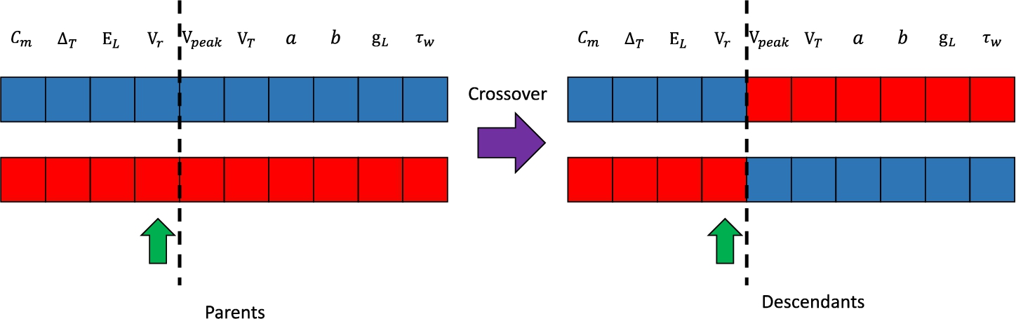
Crossover: | This step simulates sexual reproduction among those individuals previously selected to explore new regions of the search space based on the information provided by the progenitors. The process iterates through the selected individuals and pairs those at even positions with those at odd ones. For each pair, there is a user-given probability of performing single-point crossover (Salhi, 2017; Shopova and Vaklieva-Bancheva, 2006). It consists in randomly selecting a dimension of the individuals and swapping the rest of the vector between the two involved. Figure 1 depicts the single-point crossover procedure. As shown, the two progenitors (left) result in the two descendants (right) after having selected the fourth as the splitting dimension. |
Mutation: | This step tries to randomly alter the offspring that comes from the two previous ones. While crossover explores in depth the area of the search space covered by progenitors, mutation aims to allow reaching new regions of it, which avoids stagnation at local optima. The mutation procedure has a user-given probability to be launched for every individual of the offspring. Every time that it happens to apply, the individual is traversed, and each of its components has another user-given probability to be randomly reset. |
Fig. 1
Single-point crossover between two individuals.
After the three evolutionary steps described, the individuals involved are evaluated according to the objective function (only those that changed after being selected) and replace the current population for the next cycle. It is also relevant to highlight that the algorithm keeps a record with the best individuals found through the process. The solution to the problem is taken as the best one among them.
3.2Memetic Algorithm Derived from GA (MemeGA)
Memetic algorithms (Cruz et al., 2018; Marić et al., 2014) are an extension of standard genetic methods formalized by Moscato (1989). Their name comes from the term ‘meme’, defined by Dawkins (1976) as an autonomous and cultural entity similar to biological genes. However, while the individuals of genetic algorithms are mainly passive, those of memetic methods can be seen as active agents that improve their aptitude autonomously. In practical terms, this is achieved by adding the use of complementary local search techniques to the underlying process of Darwinian evolution. This approach, which is useful to avoid premature convergence while improving the exploitation of the search space, is popular in many different fields. For instance, in Marić et al. (2014), the authors design an effective and efficient parallel memetic algorithm for facility location, an NP-hard combinatorial optimization problem. A memetic algorithm is also the best-performing method for parametric heliostat field design in the study published in Cruz et al. (2018). Similarly, the optimization engine of the recent framework for drug discovery extended in Puertas-Martín et al. (2020) is a memetic method.
Considering the theoretical capabilities and the previous success cases of this kind of algorithms, a memetic method has been specifically designed and included in the present study. As introduced, the referred method is MemeGA, and it is based on the genetic method designed by Marín et al. (2020) for the problem at hand. The algorithm maintains the same structure as GA with the only exception of the mutation stage, which is replaced by the use of a local search algorithm. Namely, the original mutation probability is treated as the percentage of individuals to be randomly selected for the local search to improve them at each cycle. This approach is aligned with the proposal in Marić et al. (2014) since the local search is applied to a random subset of the population rather than to all of them, which increases diversity. As introduced, the local optimizer used is SASS, by Solis and Wets (1981), which is also the local method included in the memetic algorithms applied in Cruz et al. (2018), Puertas-Martín et al. (2020). Thus, every individual is a potential starting point for an independent execution of SASS.
As a method, SASS is a stochastic hill-climber with an adaptive step size that starts at a certain point of the search space, x. At the beginning of every iteration, SASS generates a new point,
(4)
Having generated
In contrast to the bias vector, the standard deviation of perturbation is not modified after every iteration but considering consecutive failures or successes for stability. Namely, if the number of consecutive successful iterations reaches a user-given parameter, Scnt, σ is expanded by a factor
SASS executes as many iterations, i.e. attempts to modify its current solution, as it can perform according to the number of objective function evaluations allowed by the user. After this process, the current solution of the method is finally returned. Under no circumstance will it move to a worse solution in the search space. Hence, the result of SASS will be the same initial point or a better one in the worst and best scenarios, respectively.
3.3Differential Evolution (DE)
DE is a simple yet powerful genetic-like numerical optimizer that was proposed by Storn and Price (1997) and has become widely used (Dugonik et al., 2019; Price et al., 2006). It maintains a user-defined number (NP) of randomly-generated candidate solutions (individuals) and progressively alters them to find better ones. Like GA, every individual is a vector with a valid value for each optimization variable. The workflow of this method does not try to imitate aspects such as the selection of progenitors and sexual reproduction as closely as standard genetic methods like GA. However, the terminology of DE also comes from traditional Genetic Algorithms, so each iteration applies mutation, crossover, and selection stages to every individual.
The step of mutation follows (5) to compute for each individual
(5)
The step of crossover merges each candidate solution,
(6)
Additionally, there exists an additional stage that can be linked to crossover. It is a probabilistic random-alteration process proposed by Cabrera et al. (2011) to define a variant of DE aimed at mechanism synthesis. However, the addition is not limited to that field but is of general-purpose in reality. It entails an in-breadth search component that increases variability and is similar to the traditional mutation phase of genetic algorithms such as GA. This addition aims to help the algorithm to escape from local optima, especially when working with small populations. In practical terms, it follows (7) to make more changes to each trial vector. According to it, each i component of the input trial vector can be randomly redefined around its current value with a user-given probability. The origin of the components, i.e. the current individual or its associated mutant vector, is not relevant. Therefore, this stage only adds two expected parameters: the per-component mutation probability,
(7)
After the previous steps, DE evaluates each trial vector as a solution according to the objective function. Only those trial vectors that outperform the candidate solutions from which they come persist and replace the original individuals. This process defines the population for the next iteration. DE concludes after having executed the user-defined number of iterations. At that point, the algorithm returns the best individual in the population as the solution found.
3.4Teaching-Learning-Based Optimization (TLBO)
TLBO is a recent numerical optimization method proposed by Rao et al. (2012). As a population-based meta-heuristic, this algorithm also works with a set of randomly-generated candidate solutions. However, instead of representing a group of individuals that evolve through sexual reproduction like the previous method, TLBO treats the set of solutions as a group of students. The algorithm simulates their academic interaction, considering a teacher and plain pupils, to find the global optimum of the problem at hand. This optimizer has attracted the attention of many researchers in different fields, from Engineering to Economics, because of its simplicity, effectiveness and minimalist set of parameters (Cruz et al., 2017; Rao, 2016).
The algorithm only requires two parameters to work, namely, the population size and the number of iterations to execute. Based on this information, TLBO first creates and evaluates as many random candidate solutions or individuals as indicated by the population size. As it occurs with the previous method, every individual is a plain vector containing a valid value for each optimization variable of the objective function. After this initial step, TLBO executes as many iterations as required, and every one consists of the teacher and learner phases.
The teacher phase models the way in which a professor improves the skills of his/her students. In practical terms, this step tries to shift each candidate solution towards the best one in the population, which becomes the teacher, T. After having identified that reference solution, TLBO computes the vector M. Every i component in M results from averaging those of the individuals in the current population. This information serves to create an altered or shifted solution,
(8)
The learner phase simulates the interaction between students to improve their skills. At this step, TLBO pairs every student, S, with any other different one, W. The goal is to generate a modified individual,
(9)
Additionally, although it is usually omitted, there is also an internal auxiliary stage to remove duplicate solutions in the population (Waghmare, 2013). At the end of every iteration, duplicity is avoided by randomly altering and re-evaluating any of the involved candidate solutions. Finally, after the last iteration, TLBO returns the best solution in the population as the result of the problem at hand.
3.5 Multi-Start Single-Agent Stochastic Search (MSASS)
The Multi-Start Single-Agent Stochastic Search, as introduced, consists in the inclusion of the SASS algorithm (already described as part of MemeGA in Section 3.2) within a standard multi-start component (Redondo et al., 2013; Salhi, 2017). The former is a simple yet effective local search method that will always try to move from a starting point to a nearby better solution. The latter is in charge of randomly generating different initial points, provided that the computational effort remains acceptable.
Considering the local scope of SASS, the multi-start component serves to escape from local optima by focusing the local exploration on different regions of the search space. Namely, at each iteration, the multi-start module randomly defines a feasible point. It then independently starts SASS from there. Once the local search has finished, so does the iteration, and the process is repeated from a new initial point while keeping track of the best solution found so far, which will be finally returned as the result. As a compound method, MSASS works until consuming a user-given budget of objective function evaluations.
The multi-start component expects from the user the total number of function evaluations allowed. It will always launch SASS with its maximum number of evaluations set to the remainder to consume all the budget, and the rest of its traditional parameters as defined by the user (see Section 3.2). However, in this context, SASS is enhanced with an extra parameter, i.e. the maximum number of consecutive failures that force the method to finish without consuming all the remaining function evaluations. By proceeding this way, once SASS has converged to a particular solution, the method will not waste the rest of the evaluations. Instead, it will be able to return the control to the multi-start component to look for a new start. This aspect is of great importance to increase the probabilities of finding an optimal solution.
4Experimentation and Results
4.1Environment and Configuration
The present study inherits the technical framework defined by the reference work in Marín et al. (2020). Consequently, the GrC model is simulated with the neural simulation tool NEST (Plesser et al., 2015), in its version 2.14.0, and using the 4th-order Runge-Kutta-Fehlberg solver with adaptive step-size to integrate the differential equations. The cost function, known as FF4 in the reference work as introduced, is implemented in Python (version 2.7.12) and linked to the NEST simulator. The simulation environment uses a common and fixed random-generation seed to define a stable framework and homogenize the evaluations. In this context, the GA method by Marín et al. (2020) was also implemented in Python 2.7.12 using the standard components provided by the DEAP library (Kim and Yoo, 2019).
Marín et al. configured their GA method to work with a population of 1000 individuals for 50 generations and selection tournaments of size 3. They adjusted the crossover, mutation, and per-component mutation probabilities to 60%, 10%, and 15%, respectively. Approximately, this configuration results in 30 000 evaluations of the objective function (f.e.) and also defines a general reference in computational effort. This aspect is especially relevant since the development and execution platforms differ from the original work. Namely, the four new optimizers compared (MemeGA, DE, TLBO, and MSASS) run in MATLAB 2018b after having wrapped the objective function of Marín et al. to be callable from it. The experimentation machine features an Intel Core i7-4790 processor with 4 cores and 32 GB of RAM.
The comparison takes into account four different computational costs in terms of the reference results: 50%, 75%, 100%, and 200% of the function evaluations consumed by GA, i.e. 15 000, 22 500, 30 000, and 60 000, respectively. Nevertheless, before launching the final experiments, the population-based optimizers have been tested under different preliminary configurations to find their most robust set of parameters. After having adjusted them, the focus was moved to those parameters directly affecting the overall computational cost, i.e. function evaluations. In practical terms, those are limited to the population sizes and the number of cycles for DE and TLBO. Similarly, they are the only parameters of the reference method, GA, that have been ultimately re-defined to encompass the new execution cases. However, for its memetic version, MemeGA, the number of objective function evaluations for each independent local search (local f.e.) has also been varied with the computational cost. In contrast to them, MSASS is directly configured in terms of function evaluations. Its local search component has kept the constant configuration explained below.
Table 2
Varied parameters for each population-based method and computational cost.
| Computational cost (f.e.) | |||||
| Method | Parameters | 15k | 22.5k | 30k | 60k |
| GA | Population | 1500 | 1500 | 1000 | 1000 |
| Cycles | 16 | 25 | 50 | 100 | |
| MemeGA | Population | 500 | 500 | 300 | 300 |
| Local f.e. | 10 | 12 | 20 | 35 | |
| Cycles | 20 | 26 | 40 | 50 | |
| DE | Population | 250 | 250 | 200 | 150 |
| Cycles | 60 | 90 | 150 | 400 | |
| TLBO | Population | 250 | 250 | 200 | 150 |
| Cycles | 30 | 45 | 75 | 200 | |
Table 2 shows the previous information for each population-based optimizer and computational cost. Concerning the population sizes, the general paradigm followed opted for spawning larger populations with the lower computational costs to increase and speed up the exploration. More precisely, when the computational cost is below 100% of the reference method, the population is larger to accelerate the identification of promising regions in the search space and to compensate for the impossibility of allowing the optimizer to run more cycles. Numerically, the population sizes of GA remain in the range of the reference paper for the most demanding cases and get an increment of 50% for the others. Those of MemeGA come from GA but are approximately divided by 3 to allow for the function evaluations of its independent instances of SASS, which grow from 10 to 35 for the 60k configuration. The population sizes of DE are in the range of multiplying by ten the number of variables, as suggested by the authors, and doubled to maximize diversity. TLBO successfully shares the same strategy.
Regarding the number of cycles, it is adapted from the corresponding population size to achieve the desired computational effort. GA has statistical components, but its approximate number of function calls is 60% of the population size each cycle. MemeGA keeps the crossover and mutation probabilities of GA and redefines the latter as the percentage of individuals to be locally improved. Hence, it approximately executes 60% of the population size plus 10% of the referred value multiplied by the number of local evaluations each cycle. DE consumes as many f.e. as individuals per cycle, and TLBO takes twice. The cost of evaluating the initial populations is neglected.
Concerning the rest of the parameters that have been fixed, the internal SASS component of MemeGA considers
4.2Numerical Results
Table 3 contains the results achieved by each method. There is a column for every optimizer, and each one consists of groups of cells that cover the different scenarios of computational cost. The algorithms have been independently launched 20 times for each case considering their stochastic nature, i.e. their results might vary even for the same problem instance and configuration. The referred table includes the average (ave.) and standard deviation (STD) of each case. Since the problem addressed is of minimization, the lower the values are, the better result they represent. The best average of each computational cost is in bold font. Notice that the results of GA and 30 000 f.e. (i.e. 100%) combine the five ones obtained by Marín et al. (2020) plus the remaining executions to account for 20 cases in total. Finally, to orientate the readers about the real computational cost, it is interesting to mention that completing each cell of 15 000 f.e. approximately takes 9 hours in the experimentation environment and scales accordingly.
Table 3
Objectivefunction values achieved for each compared optimizer.
| Effort (f.e.) | GA | MemeGA | DE | TLBO | MSASS |
| 15 000 (50%) | Ave.: 115.38 | Ave.: 113.51 | Ave.: 115.78 | Ave.: 105.76 | Ave.: 106.88 |
| STD: 4.19 | STD: 10.83 | STD: 7.38 | STD: 5.90 | STD: 4.50 | |
| 22 500 (75%) | Ave.: 110.32 | Ave.: 111.46 | Ave.: 112.18 | Ave.: 104.61 | Ave.: 104.71 |
| STD: 5.98 | STD: 8.03 | STD: 5.96 | STD: 7.09 | STD: 5.29 | |
| 30 000 (100%) | Ave.: 108.70 | Ave.: 103.45 | Ave.: 107.98 | Ave.: 98.63 | Ave.: 101.20 |
| STD: 6.59 | STD: 4.47 | STD: 4.74 | STD: 5.97 | STD: 3.52 | |
| 60 000 (200%) | Ave.: 104.17 | Ave.: 100.06 | Ave.: 99.44 | Ave.: 97.67 | Ave.: 100.52 |
| STD: 6.70 | STD: 5.60 | STD: 4.08 | STD: 3.37 | STD: 3.04 |
4.3Discussion
From the results in Table 3, it is possible to make several overall appreciations. Firstly, none of the optimizers stably converges to a single global solution even after doubling the computational effort allowed in the reference paper. This aspect indicates that the search space is hard to explore and features multiple sub-optimal points. For this reason, ensuring stable and global convergence might not be feasible in a reasonable amount of time. Fortunately, it is not a requirement in this context as long as the found configurations make the simulated neurons behave as expected. Secondly, all the optimizers tend to improve the average quality of their results when the computational cost increases, but TLBO always achieves the best average quality. It is also the method that has found the best individual solution known so far, with a value of 87.45. Thirdly and last, the reduction in standard deviations is not as regular as that of the averages, but for most methods, the standard deviation of the results after 60 000 f.e. is approximately half of that observed for 15 000 f.e. The only exception is the reference optimizer, GA, whose STD was better for the lightest configuration than for the heaviest. Hence, in general, the probability of obtaining particularly divergent results in quality is reduced when the optimizers are provided with enough computational budget.
As previously commented, all the methods provide better average results after increasing the computational budget, but they effectively evolve at different rates. Certainly, the average quality achieved by a certain optimizer with a particular computational cost turns out to be nearly equivalent to that of another one. Nevertheless, some of the algorithms require more computational effort to be at the same level as others. For instance, the average of GA for 60 000 f.e. is very similar to those of MSASS and TLBO for 22 500 f.e. In fact, between 15 000 and 30 000 f.e., MSASS and TLBO are a step beyond the rest. Moreover, not all the methods ultimately achieve the same degree of quality. More specifically, for 60 000 f.e., MemeGA, DE and MSASS perform similarly, but GA is worse than them, and TLBO remains numerically ahead. Thus, according to the computational cost, some of the methods stand out from the rest. TLBO and MSASS do it positively with the best averages, and GA does it negatively considering the two heaviest configurations. Regarding MemeGA and DE, the former starts to outperform the reference method with 30 000 f.e., and the latter does it after doubling this value.
After the preliminary analysis, it is necessary to test whether the methods exhibit statistically significant differences considering the impact of uncertainty. For this reason, the individual results have been studied according to the Kruskal-Wallis test (Kruskal and Wallis, 1952; Mathworks, 2021), which is a non-parametric method for testing whether the samples come from the same distribution. By proceeding this way, it is possible to assess if the results registered for each optimizer and cost seem to significantly differ from each other with reduced datasets and without making distribution assumptions. The overall significance of the tests is 0.05, i.e. the corresponding confidence level is 95%.
Observing in depth the results in Table 3 for the lightest computational cost, it seems that there are two groups. Specifically, TLBO and MSASS exhibit the best performance with close values between them, while GA, MemeGA, and DE show worse averages (and also numerically similar between them). According to the Kruskal-Wallis test, there is no significant statistical difference within each group either. Thus, for 15 000 f.e., TLBO and MSASS return indistinguishable results within a significance of 0.05. In other words, for half of the computational budget of the reference work, TLBO and MSASS are equivalent according to the results achieved. Moreover, both perform better than the rest with a statistically significant difference, including the reference method, GA. Analogously, the performances of GA, MemeGA, and DE are equivalent in this context, so there is no more expected difference than the effect of uncertainty between the three. Additionally, the fact that the memetic variant of GA, MemeGA, does not significantly outperform it can be attributed to the lack of computational budget to let local search be effective.
For 22 500 f.e., the previous situation persists: TLBO and MSASS define the group of the best-performing optimizers, without significant difference between using one or the other. GA, MemeGA, and DE remain the worst-performing methods without practical difference between them. However, for 30 000 f.e., the situation changes: MemeGA moves from the group of GA and DE to that of TLBO and MSASS, which feature the best average. At this point, the methods achieving the worst results are GA and DE, which keep being statistically indistinguishable. Those with better performance are now TLBO, MSASS, and MemeGA. Among them, TLBO and MSASS keep being statistically indistinguishable within a significance of 0.05, but the same occurs between MemeGA and MSASS. Finally, the previous trend is confirmed with 60 000 f.e: another method, DE, separates from the reference one, GA, and outperforms it. Therefore, GA persists as the only member of worse-performing methods in the end, while MemeGA, DE, TLBO, and MSASS become statistically indistinguishable between them and achieve better results than the reference method.
Based on the previous analysis, TLBO and MSASS are the best choices for 50 and 75% of the function evaluations allowed in the reference paper. For the same computational budget considered by Marín et al. (2020), the performance of MemeGA reaches the level of those two referred methods, which remain ahead. Finally, with the highest computational cost, MemeGA, DE, TLBO, and MSASS significantly outperform the reference method, and there is no meaningful difference between the four. Thus, the reference method, GA, is always outperformed by at least TLBO and MSASS. MemeGA and DE also tend to separate from it to join the other two at 30 000 and 60 000 f.e., respectively.
Additionally, for the sake of completeness, the significance of the difference between the results of each method has also been systematically assessed with the Kruskal-Wallis test under the previous significance level. According to the study, there is no statistically significant difference between the results of GA after 22 500 and 30 000 f.e. Hence, it seems possible to reduce the computational effort in the reference work by 25% without expecting worse results for any cause apart from stochasticity. TLBO, MemeGA and DE experience the same phenomenon, but they do between 15 000 and 22 500 f.e, while the performance of the last two is still similar to that of GA. Finally, MSASS stagnates between 30 000 and 60 000 f.e., which is well aligned with its conceptual simplicity and lack of sophisticated components to globally converge.
4.4Insight into the Best Solution
To conclude this section, the best result found will be analysed with further details in Fig. 2. The best-fitted neuron model according to all the features (with the lowest score) is an individual obtained by TLBO featuring a quality of 87.45 (blue lines). The neuron model from the reference work (GA optimizer) (Marín et al., 2020) with a score of 104.24 is also compared (orange lines). Finally, the in vitro data used to define the fitness function are also represented (black dots) (D’Angelo et al., 2001; Masoli et al., 2017).
Fig. 2
Spiking properties predicted by the best-fitted cerebellar granule cell (GrC) model obtained by TLBO optimizer. Simulated features and electrophysiological traces of the best solution from TLBO (blue) and compared to the neuron model from the reference work (orange) and the target in vitro recordings used in the fitness function (black dots). A) Spiking resonance curves of the models computed as average burst frequencies in response to sinusoidal stimulation of 6 pA (left) and 8 pA (right) with increasing frequencies (in steps of 0.5 Hz). B) Membrane potential evolution of the TLBO model generates spike bursts in response to sinusoidal current injections with offset of 10 pA and amplitude of 6 pA. This is shown after 2 s of stimulation (stabilization). C) Repetitive spike discharge (intensity-frequency curves) of the models computed as the mean frequency in response to step-currents of 1 s. D) Latency to the first spike in response to step-currents of 1 s. E) Membrane potential traces of the TLBO model in response to step-current injections of 1 s with various amplitudes.
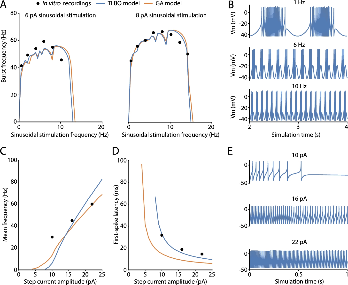
The selected neuron model has successfully captured the well-demonstrated features of the intrinsic excitability of cerebellar GrCs, i.e. repetitive spike discharge in response to injected currents (implemented as the mean frequency), latency to the first spike upon current injection (implemented as the time to the first spike), and spiking resonance in the theta-range (implemented as the average burst frequencies in response to sinusoidal stimulations). The neuron model resonates in the theta frequency band as expected, i.e. 8–12 Hz (Fig. 2(A)). The model practically reproduces identical resonance curves as the model of reference (GA model) (Marín et al., 2020). These resonance curves are the graphical representation of doublets, triplets, or longer bursts of spikes generated when stimulated by just-threshold sinusoidal stimulation at different frequencies (Fig. 2(B)). The main behaviour of biological GrCs is the increase of spike frequency when the latency to the first spike decreases as current injections increase. A sample of the neuron behaviour from which these features are calculated is shown in Fig. 2(E). The repetitive spike discharge of the TLBO model is similar to that of the model of reference and in accordance with the experimental measurements in real cells (Fig. 2(C)). The real improvement obtained by the neuron model of the proposed optimizer lies in the first-spike latency feature. The model from the reference work exhibited longer latencies than those experimentally reported, mainly with low stimulation currents (Fig. 2(D)). However, the TLBO model achieves an adjustment in its score of 7.95 ms compared to the 34.95 ms-error obtained by the GA model, both with respect to the in vitro data. Thus, the TLBO optimizer proves not only to be effective in fitting the model parameters to diverse spiking features, but also to improve both the quantitative and qualitative predictions of these supra-threshold characteristics against the methodology of reference (GA).
5Conclusions and Future Work
This article has studied the optimization component of a recent methodology for realistic and efficient neuron modelling. The referred method focuses on single-neuron processing, relies on the use of the adaptive-exponential integrate-and-fire (AdEx) model, and has been applied to cerebellar granule cells. It requires fitting its parameters to mimic experimental recordings, which can be defined as an optimization problem of ten variables. The original paper implemented a traditional genetic algorithm (GA) to address the resulting problem. This work has compared that optimizer to four alternatives: an ad-hoc memetic version of the referred genetic algorithm (MemeGA), Differential Evolution (DE), Teaching-Learning-Based Optimization (TLBO), and a multi-start method built on the same local optimizer used for MemeGA (MSASS).
All of the methods are stochastic heuristic algorithms based on solid principles that exhibit high success rates in different problems, which is why they have been selected. The comparison has been performed in terms of the context defined by the reference paper. It has considered four computational budgets for the problem resolution: 50, 75, 100, and 200% of that invested in the referred work. The effect of stochasticity at optimization has been considered by making 20 independent executions for each method and computational budget. Moreover, the assessment has not been limited to comparing their average quality. It has been complemented by studying whether the different sets of results significantly differ according to the Kruskal-Wallis test.
The original hypothesis for this work was that the optimization engine defined for the referred method could be improved, and it has been confirmed. The reference optimizer is outperformed by some of the candidates in all the scenarios, while the others equal it at least. Moreover, they tend to positively differentiate from GA as the computational budget increases. Namely, either TLBO or MSASS is equally the best choice for 15 000 and 22 500 function evaluations. Once the computational budget is the same as in the reference work, i.e. 30 000 function evaluations, MemeGA joins TLBO and MSASS. Before that point, there were no enough function evaluations to fully exploit the theoretical advantage of using a dedicated local search component over its original version. Then, no unambiguous evidence support one of them over the other two, but the three outperform GA and DE in that scenario. Ultimately, with 60 000 f.e., DE also achieves better results than GA and merges itself with TLBO, MSASS and MemeGA.
The real benefit of increasing the computational cost has also been separately studied. According to the analysis performed, the results achieved by the reference method do not significantly vary between 22 500 and 30 000 function evaluations, so the computational cost of just applying GA can be reduced by 25% without expecting a reduction in its performance. Regarding MemeGA, DE, and TLBO, they experience the same situation between 15 000 and 22 500 function evaluations. Similarly, the computational effort if using any of them could be reduced by 25% without executing more than 15 000 evaluations (logically, unless the budget can reach 30 000). Concerning MSASS, this phenomenon occurs between 30 000 and 60 000 evaluations. In this situation, 50% of the computing time could be saved by not doubling the budget for this method.
Additionally, the best configuration known so far has been found at experimentation. TLBO is the method that achieved it, and the resulting model features higher temporal accuracy of the first spike than that of the reference paper. This aspect is key for the reproduction of the relevant properties that could play a role in neuronal information transmission. This finding supports the relevance of using an effective and efficient optimization engine in the referred methodology. The gain in biological realism in simple neuron models is expected to allow the future simulation of networks compounded of thousands of these neurons to better mimic the biology. Obtaining more realistic yet efficient neuron models also allows research at levels in which in vitro or in vivo experimental biology is limited. Thus, simulations of sufficiently realistic neuronal network models can become valid to shed light on the functional roles of certain neuronal characteristics or on the interactions that may have various mechanisms among each other.
In future work, the existence of multiple sub-optimal solutions will be further studied. For that purpose, the aim is to use a state-of-the-art multi-modal optimization algorithm that can keep track of the different regions throughout its execution. That study might identify patterns that allow reducing the search space proposed in the reference work.
Acknowledgements
The authors would like to thank R. Ferri-García, from the University of Granada, for his advice on Statistics. The results included in this article are part of Milagros Marín’s PhD thesis.
References
1 | Barranca, V.J., Johnson, D.C., Moyher, J.L., Sauppe, J.P., Shkarayev, M.S., Kovačič, G., Cai, D. ((2014) ). Dynamics of the exponential integrate-and-fire model with slow currents and adaptation. Journal of Computational Neuroscience, 37: (1), 161–180. |
2 | Boussaïd, I., Lepagnot, J., Siarry, P. ((2013) ). A survey on optimization metaheuristics. Information Sciences, 237: , 82–117. |
3 | Brette, R., Gerstner, W. ((2005) ). Adaptive exponential integrate-and-fire model as an effective description of neuronal activity. Journal of Neurophysiology, 94: (5), 3637–3642. |
4 | Cabrera, J.A., Ortiz, A., Nadal, F., Castillo, J.J. ((2011) ). An evolutionary algorithm for path synthesis of mechanisms. Mechanism and Machine Theory, 46: (2), 127–141. |
5 | Cruz, N.C., Redondo, J.L., Álvarez, J.D., Berenguel, M., Ortigosa, P.M. ((2017) ). A parallel teaching–learning-based optimization procedure for automatic heliostat aiming. Journal of Supercomputing, 73: (1), 591–606. |
6 | Cruz, N.C., Redondo, J.L., Álvarez, J.D., Berenguel, M., Ortigosa, P.M. ((2018) ). Optimizing the heliostat field layout by applying stochastic population-based algorithms. Informatica, 29: (1), 21–39. |
7 | D’Angelo, E., Nieus, T., Maffei, A., Armano, S., Rossi, P., Taglietti, V., Fontana, A., Naldi, G. ((2001) ). Theta-frequency bursting and resonance in cerebellar granule cells: experimental evidence and modeling of a slow K+-dependent mechanism. Journal of Neuroscience, 21: (3), 759–770. |
8 | D’Angelo, E., Koekkoek, S.K.E., Lombardo, P., Solinas, S., Ros, E., Garrido, J., Schonewille, M., De Zeeuw, C.I. ((2009) ). Timing in the cerebellum: oscillations and resonance in the granular layer. Neuroscience, 162: (3), 805–815. |
9 | Dawkins, R. ((1976) ). The Selfish Gene. Oxford University Press, London. |
10 | Delvendahl, I., Straub, I., Hallermann, S. ((2015) ). Dendritic patch-clamp recordings from cerebellar granule cells demonstrate electrotonic compactness. Frontiers in Cellular Neuroscience, 9: , 93. |
11 | Dugonik, J., Bošković, B., Brest, J., Sepesy Maučec, M. ((2019) ). Improving statistical machine translation quality using differential evolution. Informatica, 30: (4), 629–645. |
12 | Gandolfi, D., Lombardo, P., Mapelli, J., Solinas, S., D’Angelo, E. ((2013) ). Theta-frequency resonance at the cerebellum input stage improves spike timing on the millisecond time-scale. Frontiers in Neural Circuits, 7: , 64. |
13 | Hanuschkin, A., Kunkel, S., Helias, M., Morrison, A., Diesmann, M. ((2010) ). A general and efficient method for incorporating precise spike times in globally time-driven simulations. Frontiers in Neuroinformatics, 4: , 113. |
14 | Holland, J.H. ((1975) ). Adaptation in Natural and Artificial Systems. University of Michigan Press, USA. |
15 | Jörntell, H., Ekerot, C.F. ((2006) ). Properties of somatosensory synaptic integration in cerebellar granule cells in vivo. Journal of Neuroscience, 26: (45), 11786–11797. |
16 | Kim, J., Yoo, S. ((2019) ). Software review: DEAP (Distributed Evolutionary Algorithm in Python) library. Genetic Programming and Evolvable Machines, 20: (1), 139–142. |
17 | Kruskal, W.H., Wallis, W.A. ((1952) ). Use of ranks in one-criterion variance analysis. Journal of the American Statistical Association, 47: (260), 583–621. |
18 | Lange, W. ((1975) ). Cell number and cell density in the cerebellar cortex of man and some other mammals. Cell and Tissue Research, 157: (1), 115–124. |
19 | Lindfield, G., Penny, J. ((2017) ). Introduction to Nature-Inspired Optimization. Academic Press, USA. |
20 | Marić, M., Stanimirović, Z., Djenić, A., Stanojević, P. ((2014) ). Memetic algorithm for solving the multilevel uncapacitated facility location problem. Informatica, 25: (3), 439–466. |
21 | Marín, M., Sáez-Lara, M.J., Ros, E., Garrido, J.A. ((2020) ). Optimization of efficient neuron models with realistic firing dynamics. The case of the cerebellar granule cell. Frontiers in Cellular Neuroscience, 14: , 161. |
22 | Masoli, S., Rizza, M.F., Sgritta, M., Van Geit, W., Schürmann, F., D’Angelo, E. ((2017) ). Single neuron optimization as a basis for accurate biophysical modeling: the case of cerebellar granule cells. Frontiers in Cellular Neuroscience, 11: , 71. |
23 | Mathworks (2021). Kruskal-Wallis test. https://www.mathworks.com/help/stats/kruskalwallis.html. [Last access: March, 2021]. |
24 | Moscato, P. (1989). On evolution, search, optimization, genetic algorithms and martial arts: towards memetic algorithms. Technical report, Caltech concurrent computation program, C3P Report. |
25 | Nair, M., Subramanyan, K., Nair, B., Diwakar, S. ((2014) ). Parameter optimization and nonlinear fitting for computational models in neuroscience on GPGPUs. In: 2014 International Conference on High Performance Computing and Applications (ICHPCA). IEEE, pp. 1–5. |
26 | Naud, R., Marcille, N., Clopath, C., Gerstner, W. ((2008) ). Firing patterns in the adaptive exponential integrate-and-fire model. Biological Cybernetics, 99: (4–5), 335. |
27 | Plesser, H.E., Diesmann, M., Gewaltig, M.O., Morrison, A. ((2015) ). NEST: The Neural Simulation Tool. Springer, New York, USA, pp. 1849–1852. 978-1-4614-6675-8. https://doi.org/10.1007/978-1-4614-6675-8_258. |
28 | Price, K., Storn, R.M., Lampinen, J.A. ((2006) ). Differential Evolution: A Practical Approach to Global Optimization. Springer Science & Business Media, Germany. |
29 | Puertas-Martín, S., Redondo, J.L., Pérez-Sánchez, H., Ortigosa, P.M. ((2020) ). Optimizing electrostatic similarity for virtual screening: a new methodology. Informatica, 31: (4), 821–839. |
30 | Rao, R.V. ((2016) ). Applications of TLBO algorithm and its modifications to different engineering and science disciplines. In: Teaching Learning Based Optimization Algorithm. Springer, Switzerland, pp. 223–267. |
31 | Rao, R.V., Savsani, V.J., Vakharia, D.P. ((2012) ). Teaching–learning-based optimization: an optimization method for continuous non-linear large scale problems. Information Sciences, 183: (1), 1–15. |
32 | Redondo, J.L., Arrondo, A.G., Fernández, J., García, I., Ortigosa, P.M. ((2013) ). A two-level evolutionary algorithm for solving the facility location and design (1| 1)-centroid problem on the plane with variable demand. Journal of Global Optimization, 56: (3), 983–1005. |
33 | Salhi, S. ((2017) ). Heuristic Search: The Emerging Science of Problem Solving. Springer, Switzerland. |
34 | Schmahmann, J.D. ((2019) ). The cerebellum and cognition. Neuroscience Letters, 688: , 62–75. |
35 | Shopova, E.G., Vaklieva-Bancheva, N.G. ((2006) ). BASIC—A genetic algorithm for engineering problems solution. Computers & Chemical Engineering, 30: (8), 1293–1309. |
36 | Solis, F.J., Wets, R.J.B. ((1981) ). Minimization by random search techniques. Mathematics of Operations Research, 6: (1), 19–30. |
37 | Storn, R., Price, K. ((1997) ). Differential evolution – a simple and efficient heuristic for global optimization over continuous spaces. Journal of Global Optimization, 11: (4), 341–359. |
38 | Venkadesh, S., Komendantov, A.O., Listopad, S., Scott, E.O., De Jong, K., Krichmar, J.L., Ascoli, G.A. ((2018) ). Evolving simple models of diverse intrinsic dynamics in hippocampal neuron types. Frontiers in Neuroinformatics, 12: , 8. |
39 | Waghmare, G. ((2013) ). Comments on “A note on Teaching–Learning-Based Optimization algorithm”. Information Sciences, 229: , 159–169. |
40 | Williams, R.W., Herrup, K. ((1988) ). The control of neuron number. Annual Review of Neuroscience, 11: (1), 423–453. |


