
Electrocardiogram arrhythmia detection with novel signal processing and persistent homology-derived predictors
Abstract
Many approaches to computer-aided electrocardiogram (ECG) arrhythmia detection have been performed, several of which combine persistent homology and machine learning. We present a novel ECG signal processing pipeline and method of constructing predictor variables for use in statistical models. Specifically, we introduce an isoelectric baseline to yield non-trivial topological features corresponding to the P, Q, S, and T-waves (if they exist) and utilize the N-most persistent 1-dimensional homological features and their corresponding area-minimal cycle representatives to construct predictor variables derived from the persistent homology of the ECG signal for some choice of N. The binary classification of (1) Atrial Fibrillation vs. Non-Atrial Fibrillation, (2) Arrhythmia vs. Normal Sinus Rhythm, and (3) Arrhythmias with Morphological Changes vs. Sinus Rhythm with Bradycardia and Tachycardia Treated as Non-Arrhythmia was performed using Logistic Regression, Linear Discriminant Analysis, Quadratic Discriminant Analysis, Naive Bayes, Random Forest, Gradient Boosted Decision Tree, K-Nearest Neighbors, and Support Vector Machine with a linear, radial, and polynomial kernel Models with stratified 5-fold cross validation. The Gradient Boosted Decision Tree Model attained the best results with a mean F1-score and mean Accuracy of
1.Introduction
Cardiovascular diseases are among the leading causes of death per the World Health Organization and the Centers for Disease Control and Prevention [8,64]. Arrhythmias are heart rhythms other than normal sinus rhythm with a heart rate between 60 beats/minute and 100 beats/minute; that is, arrhythmias are heart rhythms that are either too fast, too slow, abnormal, and/or irregular. Most arrhythmias must be treated since they can either lead to 1) more chaotic electrical activity of cardiac muscle resulting in loss of cardiac output and/or 2) the formation of thromboemboli (e.g. as in atrial fibrillation) possibly resulting in stroke [40]. The overall prevalence of arrhythmias among adults is estimated to be around 2% with atrial fibrillation being among the most common arrhythmias [13,30]. The global prevalence of atrial fibrillation has been estimated to be about 0.51% [35].
The contraction and relaxation of cardiac muscle cells is driven by ion movement across cell membranes and must be coordinated in order for the heart to pump blood effectively. This ion movement is governed by an electrochemical potential comprised of 1) ion concentration gradients and 2) electric potentials. The depolarization and subsequent repolarization of cardiac muscle cells causes changes in electric potential on the body surface which can be measured non-invasively using an electrocardiogram (ECG). ECG analysis is important for accurate diagnosis, treatment, and prevention of cardiovascular diseases.
Topological data analysis (TDA) refers to a collection of methods concerned with quantifying ‘shapes’ of data which are invariant under continuous deformations such as stretching and twisting. The main tool of TDA is persistent homology which quantifies the homology of structures within the data which persist over a range of scales. Persistent homology has been applied to many tasks across various fields such as electroencephalogram analysis [3], genomics [4,7,14,37,44,50,57,63], classifying skin lesions based on images [10], and tumor segmentation on histology slides [49]. Cycle representatives – which will be described in Section 1.1 – of topological features have shown utility in various fields outside of ECG analysis such as analyzing structures on the atomic scale [47] and in structural engineering [24].
Several approaches to computer-aided ECG rhythm classification have been performed, including neural networks [5,15,17,21,25,39,46,48,51,56,61,62,66–68], wavelet transformation and independent component analysis [31,65], using higher-order statistics of wavelet-packet decomposition coefficients as features [32], and support vector machines using projected and dynamic ECG features [9]. An overview of TDA applied to cardiovascular signals has recently been performed [23]. In the field of computer-aided ECG analysis, TDA has been used to construct metrics of heart rate variability [11,20]. Additionally, the Mapper algorithm has been applied to predict the presence and severity of heart disease [2]. Computer-aided ECG rhythm classification methods which utilize TDA include neural networks with topological-based features [16,53], fractal dimension in tandem with neural networks [55], mapping ECG signals to a higher dimensional space prior to computing topological features [26,27,34,36,41], and utilizing a sliding window and Fast Fourier Transform to process the ECG signal prior to computing topological features [43]. These approaches construct topological predictor variables utilizing information directly derived from the birth and death radii statistics along with extra information such as heart rate, fractal dimension statistics, and persistent entropy.
To the author’s knowledge, constructing predictor variables for use in machine learning models to classify ECG rhythms based off information derived from cycle representatives has not yet been performed. Additionally, to our knowledge, there has been no computer-aided ECG analysis which utilizes only the N-most persistent topological features for use in rhythm classification, nor has there been an approach which introduces an isoelectric baseline into ECG signals to yield non-trivial topological features corresponding to P, Q, S, and T-waves (if they are present to begin with). Introducing an isoelectric baseline prior to computing persistent homology and utilizing the N-most persistent topological features and properties of their area-minimal cycle representatives for use in constructing predictor variables makes the approach taken here distinct from other combinations of TDA and machine learning described in the literature.
In Section 1.1, we give a brief overview of the aspects of persistent homology utilized in this study. Appendix A formalizes the intuition underlying persistent homology described in Section 1.1. The Methods portion is split into three parts: Section 2.1 describes the novel ECG processing pipeline, Section 2.2 describes the construction of predictor variables primarily based off the topological features of the processed ECG signal, and Section 2.3 describes the specific classification tasks along with the statistical models and evaluation metrics used. The Results/Discussion section presents the evaluation metrics and ROC curves for each statistical model used. The Conclusion section contains a brief comparison between the method proposed here and other methods which use TDA and machine learning for rhythm classification in addition to describing some future directions.
1.1.Intuition behind persistent homology
The background on persistent homology presented both here and in Appendix A is restricted to two-dimensional data and one-dimensional homology features. The methods discussed generalize to higher dimensions, but we restrict our focus to the relevant dimensions used in the ECG analysis presented here. A toy example dataset X and its persistent homology are used to build some intuition for persistent homology. The informal treatment of persistent homology described in this section is made rigorous in Appendix A.
Fig. 1.
Example dataset with persistence diagram. A: example dataset; B–E: radius 0.57, 0.81, 1.55, and 3.01 Geometric Čech Complex depicted in black, respectively; F: persistence diagram of equivalence classes of non-contractible loops.
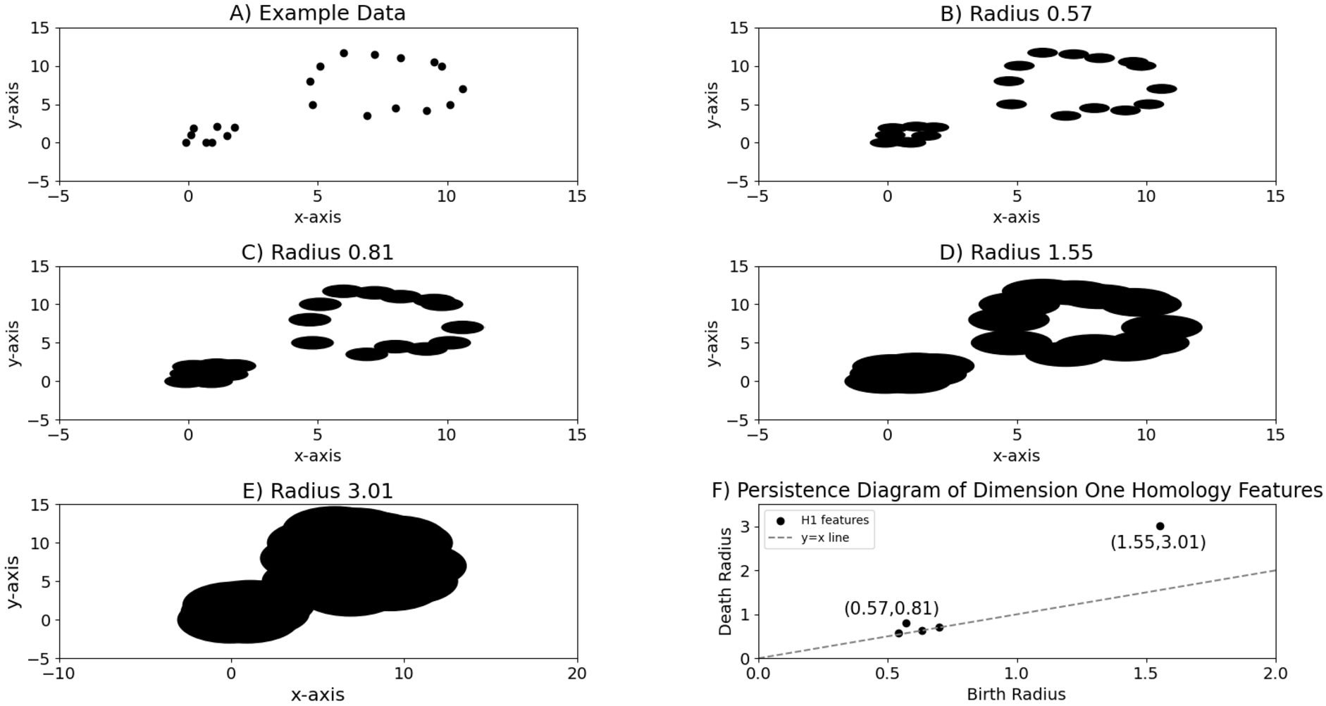
Consider the set of points in the plane
For a given two-dimensional dataset X such that there exists a non-contractible loop ℓ within
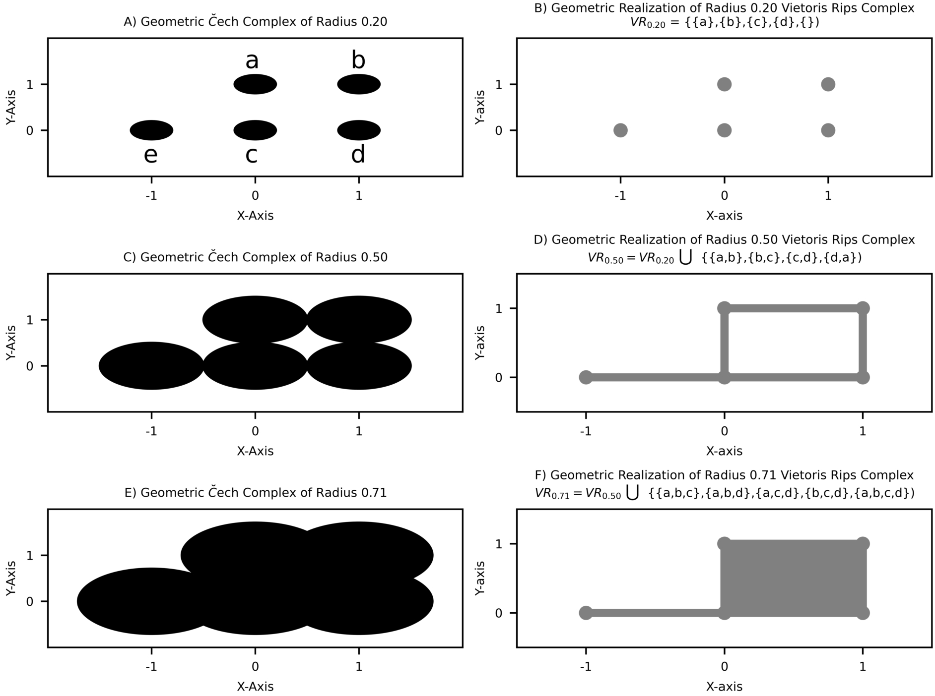
Fig. 2.
Relationship between Geometric Čech Complex of radius r and geometric realization of radius r Vietoris Rips Complex. A–C: Geometric Čech Complex of radius 0.2, 0.5, 0.71 depicted in black, respectively; D–F: geometric realization of radius 0.2, 0.5, 0.71 Vietoris Rips Complex, respectively.
The cycle representatives of a given equivalence class of non-contractible loops
2.Methods
The free and publicly available Shaoxing Hospital Zhejiang University School of Medicine electrocardiogram (ECG) database was used in this study [69]. This database consists of 10646 12-lead ECG signals, each spanning 10 seconds with a sampling frequency (i.e. the number of electric potential differences recorded per second) of 500 Hz, of which 10605 have non-empty Lead 2 signals. This study strictly utilizes Lead 2, i.e. the ‘rhythm lead’, so the term ‘ECG signal’ is henceforth used to refer to Lead 2 ECG signals. Each ECG signal is labeled with one of 11 rhythms by professional experts. The distribution of these 11 rhythms across the 10605 ECG signals is shown in Table 1.
Table 1
Rhythm distribution
| Rhythm | Count (total = 10605) | Percentage of all signals |
| Atrial Flutter | 445 | 4.20% |
| Atrial Fibrillation | 1780 | 16.78% |
| Atrial Tachycardia | 121 | 1.14% |
| Atrioventricular Node Reentrant Tachycardia | 16 | 0.15% |
| Atrioventricular Reentrant Tachycardia | 8 | 0.08% |
| Sinoatrial Block | 399 | 3.76% |
| Sinus Atrium to Atrial Wandering | 7 | 0.07% |
| Sinus Bradycardia | 3888 | 36.67% |
| Sinus Rhythm | 1826 | 17.22% |
| Sinus Rachycardia | 1568 | 14.79% |
| Supraventricular Tachycardia | 547 | 5.16% |
ECG signals are typically characterized as 1-dimensional lists of real numbers of length
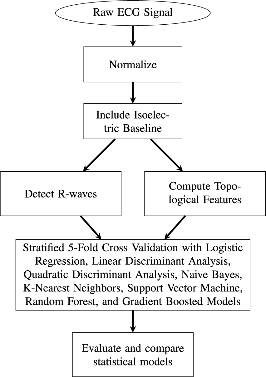
In the remainder of this section, we describe 1) ECG signal processing prior to extraction of topological features, 2) the construction of predictor variables derived from persistent homology, and 3) the statistical modeling approaches and evaluation metrics used. A flowchart providing an overview of our approach to arrhythmia detection is shown in Fig. 3.
Fig. 3.
Flowchart of ECG signal processing and arrhythmia classification.
2.1.Electrocardiogram signal processing
Given a raw ECG signal
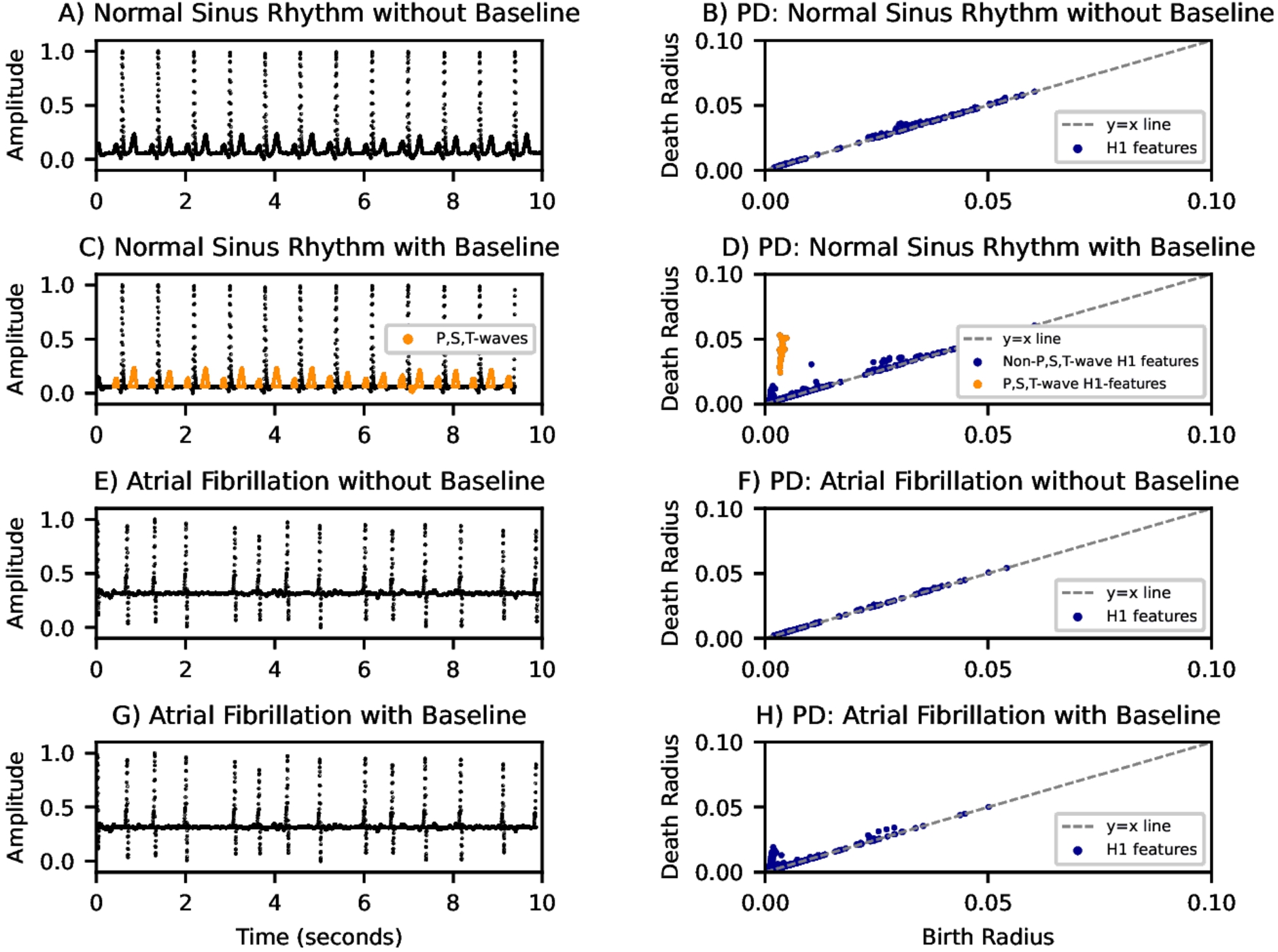
Next, an isoelectric baseline is included in
Fig. 4.
Illustration depicting the effect of the isoelectric baseline on the persistence diagrams of ECG signals. PD: persistence diagram. A–B) normal sinus rhythm ECG signal without baseline and corresponding PD. C–D) same as A–B but with the isoelectric baseline included. Note the cluster of topological features that appeared and the P, S, and T-waves their area-minimal cycle representatives correspond to. E–F) atrial fibrillation without baseline included and corresponding PD. G–H) same as E–F but with the isoelectric baseline included. H1 features: equivalence classes of non-contractible loops.
The onset of each QRS-complex in the processed ECG signal
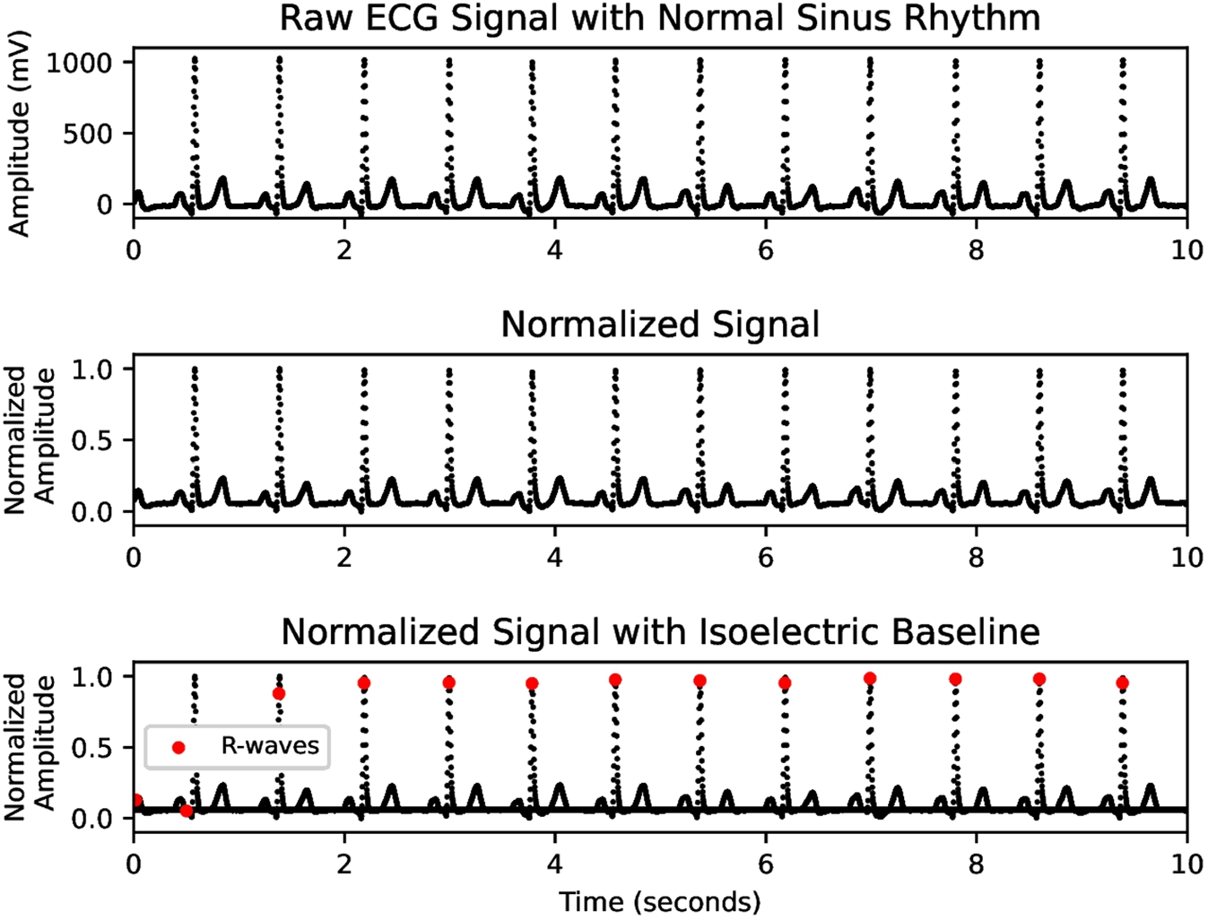
Fig. 5.
Depiction of preprocessing transformations applied to a normal sinus rhythm ECG signal. A) raw ECG signal with normal sinus rhythm. B) normalized ECG signal with maximum amplitude 1 and minimum amplitude 0. C) normalized ECG signal with isoelectric baseline included and R-waves identified.
2.2.Construction of predictor variables
Each equivalence class of non-contractible loops with birth radius b and death radius d corresponds to a set of subsets of
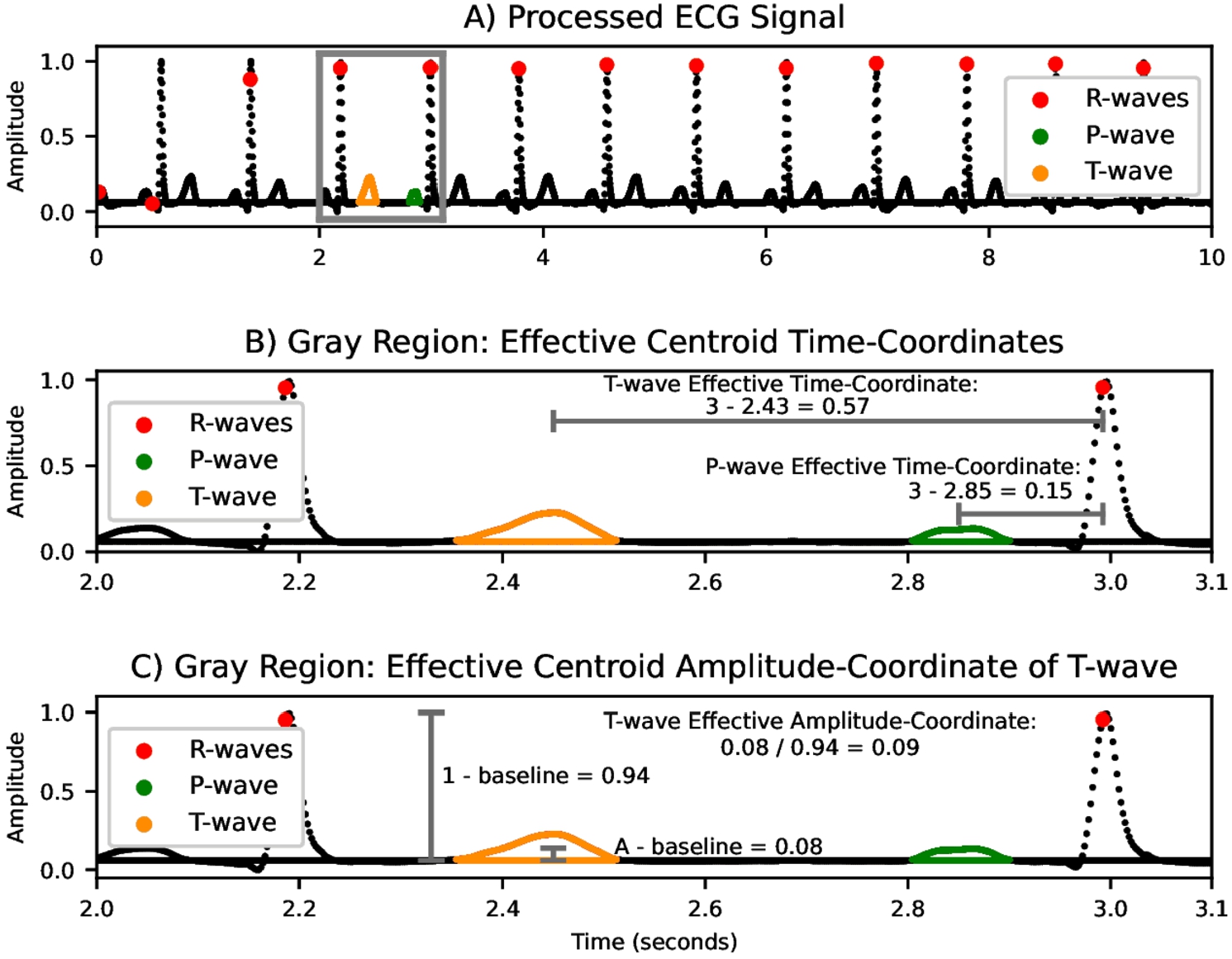
Fig. 6.
Computation of the effective centroid coordinates of an area-minimal cycle representatives. A) processed ECG signal with normal sinus rhythm and R-waves, an area-minimal cycle representative corresponding to a P-wave, and an area-minimal cycle representative corresponding to a T-wave identified. B) zoomed-in region depicting the computations of the effective time-coordinates of the two area-minimal cycle representatives. C) zoomed-in region depicting the computation of the effective amplitude-coordinate of the area-minimal cycle representative corresponding to the T-wave.
The persistent homology of the processed signal
2.3.Statistical modeling and evaluation
Three different binary classifications are carried out:
Atrial Fibrillation vs. Non-Atrial Fibrillation
Arrhythmia vs. Normal Sinus Rhythm
Arrhythmias with Morphological Changes vs. Sinus Rhythm with Bradycardia and Tachycardia Treated as Non-Arrhythmia
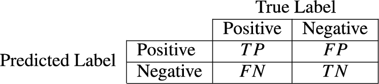
Fig. 7.
Confusion matrix.
The optimal hyperparameters for the Random Forest, Gradient Boosted Decision Tree, K-Nearest Neighbors, and Support Vector Machines with Radial and Polynomial Kernel Models were chosen as the hyperparameters which yielded the largest mean F1-Score across all folds in 5-fold stratified cross validation. The grid search spaces of hyperparameters for the relevant models are:
Random Forest:
∗
∗
Gradient Boosted Decision Tree:
∗
∗
K-Nearest Neighbors:
∗
Support Vector Machine with Radial Kernel:
∗
∗
Support Vector Machine with Polynomial Kernel:
∗
∗
3.Results/discussion
Table 2
Binary classification outcomes: atrial fibrillation vs. Non-atrial fibrillation
| Model | F1-score | Accuracy | Sensitivity | Specificity | PPV | NPV | Optimal N |
| Logistic regression | 0.938 ± 0.002 | 0.896 ± 0.004 | 0.947 ± 0.005 | 0.646 ± 0.018 | 0.930 ± 0.003 | 0.712 ± 0.018 | 24 |
| Linear discriminant analysis | 0.934 ± 0.002 | 0.890 ± 0.004 | 0.941 ± 0.004 | 0.637 ± 0.019 | 0.928 ± 0.003 | 0.686 ± 0.015 | 30 |
| Quadratic discriminant analysis | 0.917 ± 0.004 | 0.864 ± 0.008 | 0.908 ± 0.008 | 0.642 ± 0.063 | 0.927 ± 0.012 | 0.585 ± 0.019 | 25 |
| Naive Bayes | 0.890 ± 0.006 | 0.818 ± 0.009 | 0.880 ± 0.011 | 0.511 ± 0.034 | 0.899 ± 0.006 | 0.463 ± 0.024 | 5 |
| Random forest | 0.955 ± 0.004 | 0.925 ± 0.007 | 0.964 ± 0.004 | 0.734 ± 0.043 | 0.947 ± 0.008 | 0.803 ± 0.016 | 4 |
| Gradient boosted model | 0.967 ± 0.003 | 0.946 ± 0.006 | 0.959 ± 0.004 | 0.880 ± 0.019 | 0.975 ± 0.004 | 0.813 ± 0.018 | 20 |
| K-Nearest Neighbors | 0.942 ± 0.004 | 0.894 ± 0.007 | 0.925 ± 0.006 | 0.712 ± 0.021 | 0.952 ± 0.004 | 0.660 ± 0.035 | 23 |
| Support Vector Machine: linear kernel | 0.941 ± 0.003 | 0.898 ± 0.005 | 0.935 ± 0.004 | 0.706 ± 0.020 | 0.942 ± 0.006 | 0.705 ± 0.022 | 29 |
| Support Vector Machine: radial kernel | 0.927 ± 0.002 | 0.868 ± 0.003 | 0.869 ± 0.003 | 0.856 ± 0.025 | 0.991 ± 0.002 | 0.272 ± 0.016 | 5 |
| Support Vector Machine: polynomial kernel | 0.937 ± 0.004 | 0.890 ± 0.007 | 0.908 ± 0.005 | 0.749 ± 0.022 | 0.964 ± 0.002 | 0.539 ± 0.031 | 17 |
Table 3
Binary classification outcomes: arrhythmia vs. Normal sinus rhythm
| Model | F1-score | Accuracy | Sensitivity | Specificity | PPV | NPV | Optimal N |
| Logistic regression | 0.634 ± 0.019 | 0.876 ± 0.004 | 0.622 ± 0.029 | 0.929 ± 0.002 | 0.647 ± 0.009 | 0.922 ± 0.005 | 10 |
| Linear discriminant analysis | 0.629 ± 0.023 | 0.867 ± 0.008 | 0.652 ± 0.028 | 0.912 ± 0.006 | 0.607 ± 0.022 | 0.927 ± 0.006 | 20 |
| Quadratic discriminant analysis | 0.481 ± 0.012 | 0.709 ± 0.010 | 0.783 ± 0.016 | 0.694 ± 0.011 | 0.347 ± 0.010 | 0.939 ± 0.004 | 24 |
| Naive Bayes | 0.460 ± 0.010 | 0.673 ± 0.016 | 0.809 ± 0.025 | 0.644 ± 0.022 | 0.322 ± 0.010 | 0.942 ± 0.006 | 24 |
| Random forest | 0.829 ± 0.010 | 0.942 ± 0.003 | 0.812 ± 0.017 | 0.969 ± 0.003 | 0.847 ± 0.014 | 0.961 ± 0.003 | 8 |
| Gradient boosted model | 0.839 ± 0.011 | 0.946 ± 0.003 | 0.815 ± 0.019 | 0.974 ± 0.002 | 0.866 ± 0.009 | 0.962 ± 0.004 | 12 |
| K-Nearest Neighbors | 0.722 ± 0.004 | 0.899 ± 0.007 | 0.747 ± 0.006 | 0.924 ± 0.021 | 0.664 ± 0.004 | 0.964 ± 0.035 | 5 |
| Support Vector Machine: linear kernel | 0.638 ± 0.003 | 0.889 ± 0.005 | 0.743 ± 0.004 | 0.910 ± 0.020 | 0.563 ± 0.006 | 0.958 ± 0.022 | 20 |
| Support Vector Machine: radial kernel | 0.720 ± 0.002 | 0.912 ± 0.003 | 0.869 ± 0.003 | 0.918 ± 0.025 | 0.612 ± 0.002 | 0.982 ± 0.016 | 5 |
| Support Vector Machine: polynomial kernel | 0.631 ± 0.004 | 0.891 ± 0.007 | 0.797 ± 0.005 | 0.902 ± 0.022 | 0.516 ± 0.002 | 0.975 ± 0.031 | 21 |
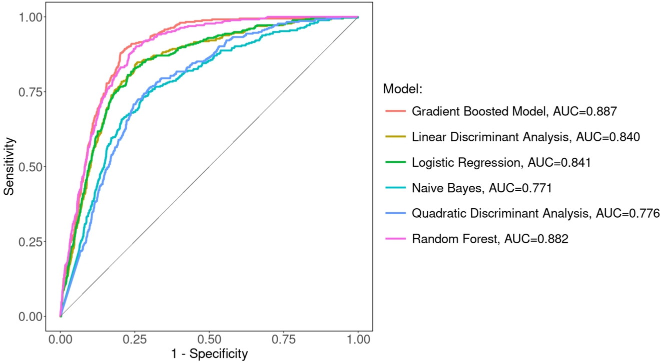
The mean and standard deviation across the five folds for the binary classifications of (i) Atrial Fibrillation vs. Non-Atrial Fibrillation, (ii) Arrhythmia vs. Normal Sinus Rhythm, and (iii) Arrhythmia with Morphological Changes vs. Sinus Rhythm with Bradycardia and Tachycardia Treated as Non-Arrhythmia with the hyperparameters yielding the largest F1-Score are shown in Tables 2, 3, and 4, respectively. The results corresponding to the top-performing model with respect to each evaluation metric are displayed in bold. Observe that the Gradient Boosted Decision Tree Model outperforms all other models with respect to F1-Score and Accuracy across each of the three binary classification tasks, closely followed by the Random Forest Model. The maximum mean F1-Score attained by the Gradient Boosted Decision Tree Model across the five folds was 0.967, 0.839, and 0.943 for binary classification of Atrial Fibrillation vs. Non-Atrial Fibrillation, Arrhythmia vs. Normal Sinus Rhythm, and Arrhythmia with Morphological Changes vs. Sinus Rhythm with Bradycardia and Tachycardia Treated as Non-Arrhythmia, respectively. The corresponding mean Accuracy attained by the Gradient Boosted Decision Tree Model across the five folds was 0.946, 0.946, and 0.921 for binary classification of Atrial Fibrillation vs. Non-Atrial Fibrillation, Arrhythmia vs. Normal Sinus Rhythm, and Arrhythmia with Morphological Changes vs. Sinus Rhythm with Bradycardia and Tachycardia Treated as Non-Arrhythmia, respectively. The Gradient Boosted Decision Tree and Random Forest models outperformed all other models with respect to the area under the Receiver-Operator Characteristic Curves (AUC) for all three classification tasks as seen in Fig. 8, Fig. 9, and Fig. 10. This may be due to heterogeneity of the data; regardless, in computer-aided ECG analysis, interpretability of statistical models may be less important than the performance of said models, rendering more support in favor of ensemble and tree-based modeling approaches given their favorable performance.
Recall that TDA quantifies the ‘shape’ of data. Thus, the motivation behind presenting the classifications of both (i) Arrhythmia vs. Normal Sinus Rhythm and (ii) Arrhythmias with Morphological Changes vs. Sinus Rhythm with Bradycardia and Tachycardia Treated as Non-Arrhythmia is to illustrate how the results are improved when TDA is used to classify two groups that primarily have different shapes, not frequencies. With this in mind, it may not be surprising that the presented TDA approach performs much better when classifying arrhythmias when the only two arrhythmias characterized solely by abnormal periodicity (assuming the individual has at most one rhythm as is the case in the data used in this study) – i.e. tachycardia and bradycardia – are not considered to be part of the arrhythmia group.
Table 4
Binary classification outcomes: arrhythmia with morphological changes vs. Sinus rhythm with bradycardia and tachycardia treated as non-arrhythmia
| Model | F1-score | Accuracy | Sensitivity | Specificity | PPV | NPV | Optimal N |
| Logistic regression | 0.904 ± 0.002 | 0.865 ± 0.004 | 0.932 ± 0.003 | 0.717 ± 0.011 | 0.878 ± 0.004 | 0.828 ± 0.007 | 30 |
| Linear discriminant analysis | 0.905 ± 0.002 | 0.866 ± 0.003 | 0.927 ± 0.007 | 0.734 ± 0.012 | 0.884 ± 0.004 | 0.821 ± 0.012 | 30 |
| Quadratic discriminant analysis | 0.857 ± 0.004 | 0.797 ± 0.003 | 0.884 ± 0.014 | 0.607 ± 0.025 | 0.831 ± 0.007 | 0.706 ± 0.018 | 25 |
| Naive Bayes | 0.859 ± 0.004 | 0.794 ± 0.006 | 0.912 ± 0.008 | 0.536 ± 0.013 | 0.812 ± 0.005 | 0.735 ± 0.018 | 27 |
| Random forest | 0.933 ± 0.005 | 0.906 ± 0.007 | 0.952 ± 0.005 | 0.805 ± 0.012 | 0.915 ± 0.005 | 0.885 ± 0.012 | 10 |
| Gradient boosted model | 0.943 ± 0.004 | 0.921 ± 0.006 | 0.955 ± 0.004 | 0.847 ± 0.013 | 0.932 ± 0.005 | 0.896 ± 0.009 | 10 |
| K-Nearest Neighbors | 0.905 ± 0.004 | 0.861 ± 0.007 | 0.883 ± 0.006 | 0.807 ± 0.021 | 0.923 ± 0.004 | 0.741 ± 0.035 | 19 |
| Support Vector Machine: linear kernel | 0.905 ± 0.003 | 0.866 ± 0.005 | 0.886 ± 0.004 | 0.815 ± 0.020 | 0.923 ± 0.006 | 0.745 ± 0.022 | 29 |
| Support Vector Machine: radial kernel | 0.883 ± 0.002 | 0.828 ± 0.003 | 0.813 ± 0.003 | 0.896 ± 0.025 | 0.968 ± 0.002 | 0.507 ± 0.016 | 5 |
| Support Vector Machine: polynomial kernel | 0.897 ± 0.004 | 0.845 ± 0.007 | 0.848 ± 0.005 | 0.833 ± 0.022 | 0.949 ± 0.002 | 0.637 ± 0.031 | 16 |
Fig. 8.
Receiver operator characteristic curve for classification of atrial fibrillation vs. Non-atrial fibrillation.
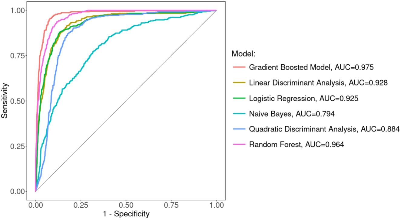
Fig. 9.
Receiver operator characteristic curve for classification of arrhythmia vs. Sinus rhythm.
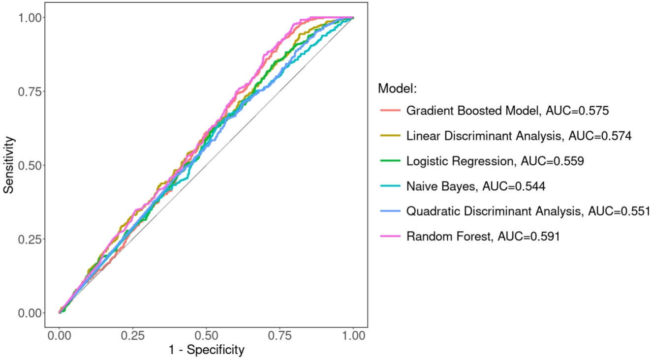
Fig. 10.
Receiver operator characteristic curve for classification of arrhythmia with morphological changes vs. Sinus rhythm with bradycardia and tachycardia treated as non-arrhythmia.
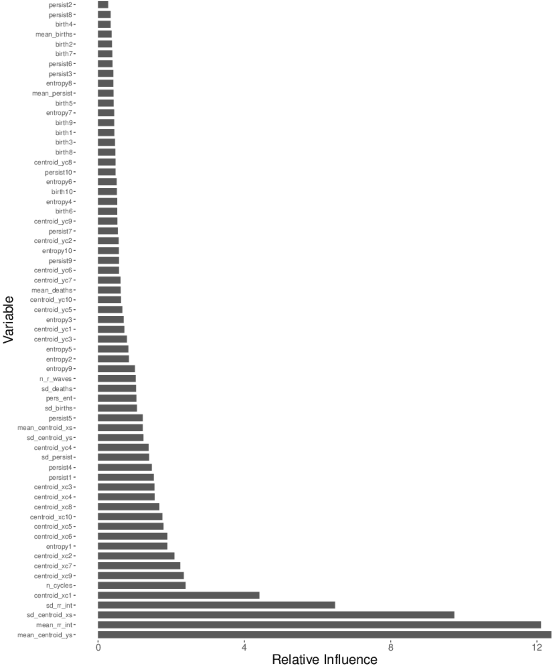
The relative influence [18] of each predictor variable in the top-performing model with respect to mean F1-score (i.e. Gradient Boosted Decision Tree model) across the five folds in the classifications of Atrial Fibrillation vs. Non-Atrial Fibrillation, Arrhythmia vs. Normal Sinus Rhythm, and Arrhythmia with Morphological Changes vs. Sinus Rhythm with Bradycardia and Tachycardia Treated as Non-Arrhythmia are shown in Fig. 11, Fig. 12, Fig. 13 in Appendix B. Atrial fibrillation is characterized by (1) absent/attenuated P-waves and (2) irregularly irregular frequency, so it is not surprising that the standard deviation of the RR-interval holds most influence for the classification of Atrial Fibrillation vs. Non-Atrial Fibrillation. Note that 9 of the 15 most influential predictor variables in the classification of Atrial Fibrillation vs. Non-Atrial Fibrillation stem from area-minimal cycle representatives and that
Table 5
Comparison of studies applying TDA and machine learning to arrhythmia classification
| Title | Database(s) | Preprocessing | Features | Model(s) |
| Topological Data Analysis for Arrhythmia Detection Through Modular Neural Networks [16] | PhysioNet MIT-BIH Normal Sinus Rhythm, Arrhythmia, Supraventricular Arrhythmia, Malignant Ventricular Arrhythmia, and Long Term Database | Resample as different frequency, remove baseline, finite impulse response filter, Kalman filter, rescale, translate | Coefficients from Discrete Fourier Transform of sliding windows; linear relationships between P, Q, R, S, & T-waves; extrema, mean, standard deviation, kurtosis, skewness, entropy, crossing-overs, PCA reduction of persistence statistics | Autoencoder |
| Nonlinear dynamic approaches to identify atrial fibrillation progression based on topological methods [55] | PhysioBank long-term atrial fibrillation database; PhysioNet MIT-BIH normal sinus rhythm database | Normalize, time-delay embedding | Number and persistence of 1-dimensional topological features and fractal dimension | Feed-forward back propagation neural network |
| Classification of Single-Lead Electrocardiograms: TDA Informed Machine Learning [26] | Alivecor | Butterworth filter and time-delay embedding | Sum, mean, standard deviation, skewness, kurtosis of birth, death, and/or persistence of 0, 1, & 2-dimensional topological features | Random forest classifier |
| Persistence Landscape-based Topological Data Analysis for Personalized Arrhythmia Classification [36] | PhysioNet MIT-BIH Long-Term database | Resample at different frequency, Butterworth filter, detect R waves and segment signal, time-delay embedding, downsample | Persistence landscape-derived statistics | Random forest classifier |
| Early Ventricular Fibrillation Prediction Based on Topological Data Analysis of ECG Signal [34] | PhysioNet CUDB, SDDB, PTBDB | Resample at different frequency, moving average filter, normalization, time-delay embedding | Sum, mean, and variance of persistences of 0, 1, & 2-dimensional topological features; box-counting features; heart rate variability features | Logistic regression, decision trees, SVM, KNN classifier |
| Ventricular Fibrillation and Tachycardia Detection Using Features Derived from Topological Data Analysis [41] | AHA 2000 series and PhysioNet MIT-BIH Malignant Arrhythmia Database | Infinite impulse response filter, time-delay embedding | Derived from representations of time domain signal, embedded signal, persistence diagram, persistence landscape representation, weighted silhouettes representation | KNN classifier |
| A Topology Informed Random Forest Classifier for ECG Classification [27] | PhysioNet/Computing in Cardiology Challenge 2020 | Time-delay embedding | Persistence entropy and statistics derived from persistence diagram and persistence landscape | Two-level random forest classifier |
| A Novel Heart Disease Classification Algorithm based on Fourier Transform and Persistent Homology [43] | PhysioNet MIT-BIH Arrhythmia Database | Butterworth filter, sliding window fast Fourier Transform to embed signal in higher dimension | Persistence entropy and persistence statistics | SVM |
The methods used in other studies that approach computer-aided ECG rhythm classification through a combination of TDA and machine learning are summarized in Table 5. Due to the wide range of classification tasks performed and evaluation metrics used in these studies, the classification tasks and evaluation metrics are not shown in Table 5 to avoid (i) presenting misleading comparisons and (ii) subjectivity in choosing the results from other studies to present. These other studies use a variety of databases [19,42] and sometimes a sample size on the scale of tens or hundreds, in addition to having longer – and consequently more informative – signals compared to the database used in this study [69]. Another factor to consider when comparing analyses of TDA and machine learning in ECG rhythm classification is the fact that different ECG databases often have signals labeled with different rhythms that may not be found in other ECG databases. The approach presented here attains similar results as these previous studies with respect to classification outcomes while utilizing a novel ECG signal processing pipeline and topological predictor variable construction, particularly with respect to using information derived from area-minimal cycle representatives.
4.Conclusion
The method presented here differs from other methods utilizing TDA and machine learning in three main ways:
by using information about optimal cycle representatives of equivalence classes of non-contractible loops when constructing topological predictor variables.
by focusing only on the N-most persistent equivalence classes of non-contractible loops when constructing topological predictor variables.
by introducing an isoelectric baseline to create non-trivial equivalence classes of non-contractible loops corresponding to the P, Q, S, and T-waves (if they are present to begin with).
There have been people working on computer-aided ECG analysis since the invention of the ECG machine. Over the past 20 years, there have been many machine learning approaches taken, yielding encouraging results. Some of these methods have involved TDA. Regardless of the type of method taken in computer-aided ECG analysis and the goodness of the evaluation metrics, we must take care to not rush to replace ECG interpretation by skilled health care professionals, however tempting the potential time and cost savings may be. In addition to the obvious danger of automated arrhythmia classification algorithms missing a harmful arrhythmia that a skilled healthcare professional would not have missed, bells and whistles from automated arrhythmia detection algorithms can lead to unnecessary medical staff fatigue and an increase in stress and adverse outcomes in hospitalized patients [12,29,33,54,58,59].
The data used in this study are free and publicly available at https://figshare.com/collections/ChapmanECG/4560497/2 [69]. The code used in this study is free and publicly available and can be found on GitHub: https://github.com/hdlugas/ekg_tda_arrhythmia_detection.
Acknowledgement
The computations of topological features and all optimal parameter searches were performed on Wayne State University’s High-Performance Computing Grid.
Appendices
Appendix A.
Appendix A.Formalization of persistent homology intuition
We now set out to formalize the notion of “equivalence classes of non-contractible loops that persist for a given range of radius values.” Given a set of data X represented as a finite set of points in
Definition A.1.
A simplicial complex is a collection K of subsets of a finite set V such that:
if
There are several ways to construct a simplicial complex given a finite set of points in
Definition A.2.
Given a dataset X represented as a finite subset of
Note that if
We are now in a position to be more concrete about the notion of an “equivalence class of non-contractible loops” within the geometric Čech complex, as discussed in Section 1.1. By an “equivalence class of non-contractible loops,” we are referring to an element of the 1-dimensional homology group of some radius r Vietoris–Rips complex, which we now set out to define.
Let X be a finite subset of
Definition A.3.
Given
By increasing r, we create a sequence of Vietoris–Rips Complexes where
Definition A.4.
Let
Up to a scaling factor in the variable r, the Geometric Čech complex of radius r is homotopy equivalent to the Radius r Vietoris–Rips complex due to the Nerve Lemma (see Corollary 4G.3 in Hatcher) [22]. Consequently, the definitions of the birth and death radius of an equivalence class of non-contractible loops presented in Section 1.1 are equivalent to the definitions of the birth and death filtration of a class
Appendix B.
Appendix B.Relative influence of predictor variables in top-performing models
Figures depicting the relative influence of the top-performing models with respect to F1-score in each of the three classification tasks are displayed. Note that for each of the three classification tasks, the top-performing model with respect to F1-score was the Gradient Boosted Decision Tree Model.
Fig. 11.
Relative influence of predictor variables in top-performing gradient boosted decision tree model in classification of atrial fibrillation vs. Non-atrial fibrillation.
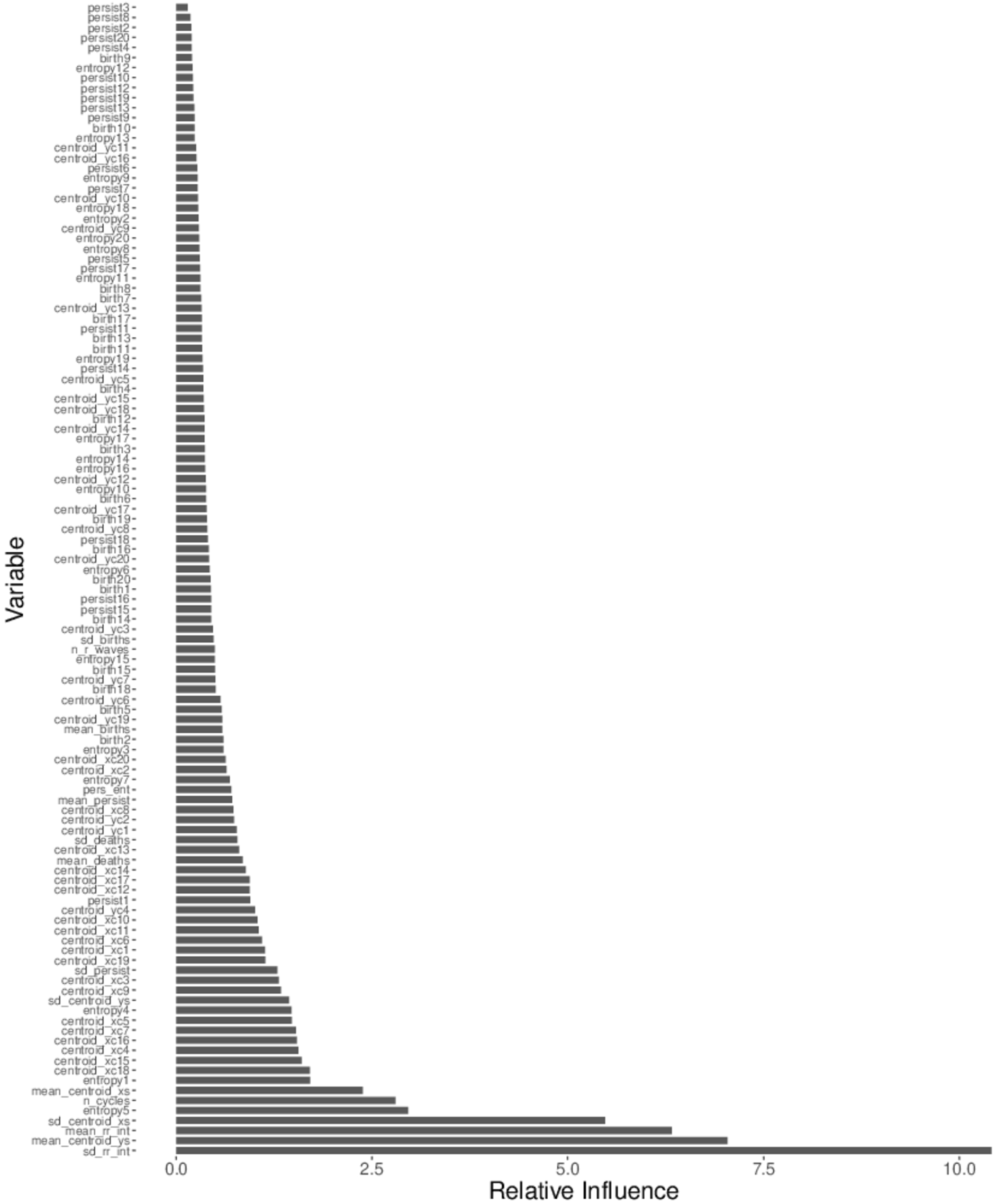
Fig. 12.
Relative influence of predictor variables in top-performing gradient boosted decision tree model in classification of arrhythmia vs. Normal sinus rhythm.
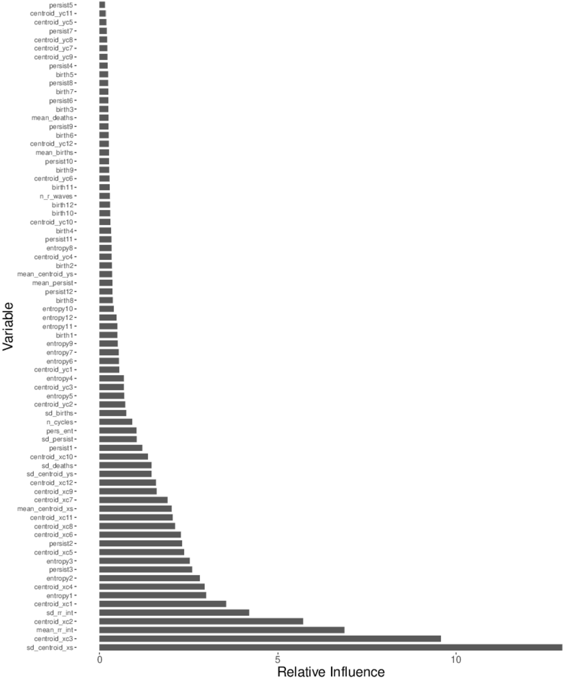
Fig. 13.
Relative influence of predictor variables in top-performing gradient boosted decision tree model in classification of arrhythmia with morphological changes vs. Sinus rhythm with bradycardia and tachycardia treated as non-arrhythmia.
References
[1] | H. Adams, T. Emerson, M. Kirby, R. Neville, C. Peterson, P. Shipman, S. Chepushtanova, E. Hanson, F. Motta and L. Ziegelmeier, Persistence images: A stable vector representation of persistent homology, J. Mach. Learn. Res. 18: ((2017) ), 218–252, https://arxiv.org/abs/1507.06217. |
[2] | A. Aljanobi and J. Lee, Topological Data Analysis for Classification of Heart Disease Data, 2021 IEEE International Conference on Big Data and Smart Computing (BigComp), Jeju Island, Korea (South), (2021) , pp. 210–213. doi:10.1109/BigComp51126.2021.00047. |
[3] | F. Altındiş, B. Yılmaz, S. Borisenok and K. İçöz, Parameter investigation of topological data analysis for EEG signals, Biomedical Signal Processing And Control. 63: ((2021) ), 102196. doi:10.1016/j.bspc.2020.102196. |
[4] | J. Arsuaga, N. Baas, D. Dewoskin, H. Mizuno, A. Pankov and C. Park, Topological analysis of gene expression arrays identifies high risk molecular subtypes in breast cancer, Appl. Algebra Eng., Commun. Comput. 23: ((2012) ), 3–15. doi:10.1007/s00200-012-0166-8. |
[5] | A. Asgharzadeh-Bonab, M. Amirani and A. Mehri, Spectral entropy and deep convolutional neural network for ECG beat classification, Biocybernetics And Biomedical Engineering. 40: ((2020) ), 691–700. doi:10.1016/j.bbe.2020.02.004. |
[6] | U. Bauer, Ripser: Efficient computation of Vietoris–Rips persistence barcodes, Journal Of Applied And Computational Topology ((2021) ), https://arxiv.org/abs/1908.02518. |
[7] | P.G. Camara, D.I. Rosenbloom, K.J. Emmett, A.J. Levine and R. Rabadan, Topological data analysis generates high-resolution, genome-wide maps of human recombination. Cell Syst. 3: (1) ((2016) ), 83–94. doi:10.1016/j.cels.2016.05.008. |
[8] | Centers for Disease Control and Prevention, Leading causes of death, https://www.cdc.gov/nchs/fastats/leading-causes-of-death.htm. |
[9] | S. Chen, W. Hua, Z. Li, J. Li and X. Gao, Heartbeat classification using projected and dynamic features of ECG signal, Biomedical Signal Processing And Control. 31: ((2017) ), 165–173. doi:10.1016/j.bspc.2016.07.010. |
[10] | Y. Chung, C. Hu, A. Lawson and C. Smyth, Topological approaches to skin disease image analysis, in: 2018 IEEE International Conference on Big Data (Big Data), (2018) , pp. 100–105. doi:10.1109/BigData.2018.8622175. |
[11] | Y. Chung, C. Hu, Y. Lo and H. Wu, A persistent homology approach to heart rate variability analysis with an application to sleep-wake classification, Frontiers In Physiology. 12: ((2021) ), 202, https://arxiv.org/abs/1908.06856. |
[12] | S.A. Dee, J. Tucciarone, G. Plotkin and C. Mallilo, Determining the impact of an alarm management program on alarm fatigue among ICU and telemetry RNs: An evidence based research project, SAGE Open Nurs. 13: (8) ((2022) ), 23779608221098713. doi:10.1177/23779608221098713. |
[13] | D.S. Desai and H.S. Arrhythmias, StatPearls [internet]. Treasure Island (FL): StatPearls publishing, (2024) . Available from: https://www.ncbi.nlm.nih.gov/books/NBK558923/. |
[14] | D. DeWoskin, J. Climent, I. Cruz-White, M. Vazquez, C. Park and J. Arsuaga, Applications of computational homology to the analysis of treatment response in breast cancer patients, Topology And Its Applications. 157: ((2010) ), 157–164. doi:10.1016/j.topol.2009.04.036. |
[15] | S. Dhyani, A. Kumar and S. Choudhury, Arrhythmia disease classification utilizing ResRNN, Biomedical Signal Processing And Control. 79: ((2023) ), 104160. doi:10.1016/j.bspc.2022.104160. |
[16] | M. Dindin, Y. Umeda and F. Chazal, Topological data analysis for arrhythmia detection through modular neural networks. Advances In Artificial Intelligence. ((2020) ). |
[17] | F. Elhaj, N. Salim, A. Harris, T. Swee and T. Ahmed, Arrhythmia recognition and classification using combined linear and nonlinear features of ECG signals, Computer Methods And Programs In Biomedicine. 127: ((2016) ), 52–63. doi:10.1016/j.cmpb.2015.12.024. |
[18] | J.H. Friedman, Greedy function approximation: A gradient boosting machine, Ann. Statist. 29: (5) ((2001) ), 1189–1232. doi:10.1214/aos/1013203451. |
[19] | A. Goldberger, L. Amaral, L. Glass, J. Hausdorff, P.C. Ivanov, R. Mark and H.E. Stanley, PhysioBank, PhysioToolkit, and PhysioNet: Components of a new research resource for complex physiologic signals, Circulation [Online] 101: (23) ((2000) ), e215–e220. doi:10.1161/01.cir.101.23.e215. |
[20] | G. Graff, Persistent homology as a new method of the assessment of heart rate variability, PLOS ONE 16: ((2021) ), 1–24. doi:10.1371/journal.pone.0253851. |
[21] | L. Guo, G. Sim and B. Matuszewski, Inter-patient ECG classification with convolutional and recurrent neural networks, Biocybernetics And Biomedical Engineering. 39: ((2019) ), 868–879, https://www.sciencedirect.com/science/article/pii/S0208521618304200. doi:10.1016/j.bbe.2019.06.001. |
[22] | A. Hatcher, Algebraic Topology, Cambridge University Press, ISBN: 9780521795401 (2002) . |
[23] | E. Hernández-Lemus, P. Miramontes and M. Martínez-García, Topological data analysis in cardiovascular signals: An overview, Entropy 26: (1) ((2024) ), 67. doi:10.3390/e26010067. |
[24] | Y. Hiraoka, T. Nakamura, A. Hirata, E. Escolar, K. Matsue and Y. Nishiura, Hierarchical structures of amorphous solids characterized by persistent homology, Proceedings Of The National Academy Of Sciences 113: ((2016) ), 7035–7040. doi:10.1073/pnas.1520877113. |
[25] | Y. Huang, H. Li and X. Yu, A novel time representation input based on deep learning for ECG classification, Biomedical Signal Processing And Control. 83: ((2023) ), 104628. doi:10.1016/j.bspc.2023.104628. |
[26] | P. Ignacio, C. Dunstan, E. Escobar, L. Trujillo and D. Uminsky, Classification of single-lead electrocardiograms: TDA informed machine learning, in: 2019 18th IEEE International Conference on Machine Learning and Applications (ICMLA), (2019) , pp. 1241–1246. doi:10.1109/ICMLA.2019.00204. |
[27] | P.S. Ignacio, J.A. Bulauan and J.R. Manzanares, in: A Topology Informed Random Forest Classifier for ECG Classification, 2020 Computing in Cardiology, Rimini, Italy, (2020) , pp. 1–4. doi:10.22489/CinC.2020.297. |
[28] | G. James, D. Witten, T. Hastie and R. Tibshirani, An Introduction to Statistical Learning with Applications in R, Springer, New York, NY, ISBN: 1461471370, (2021) . |
[29] | K.R. Johnson, J.I. Hagadorn and D.W. Sink, Alarm safety and alarm fatigue, Clin Perinatol. 44: (3) ((2017) ), 713–728. Epub 2017 Jul 14. doi:10.1016/j.clp.2017.05.005. |
[30] | S. Khurshid, S.H. Choi, L.C. Weng, E.Y. Wang, L. Trinquart, E.J. Benjamin, P.T. Ellinor and S.A. Lubitz, Frequency of cardiac rhythm abnormalities in a half million adults. Circ Arrhythm Electrophysiol. 11: (7) ((2018) ), e006273. doi:10.1161/CIRCEP.118.006273. |
[31] | M. Kumar, R. Pachori and U. Rajendra Acharya, Automated diagnosis of atrial fibrillation ECG signals using entropy features extracted from flexible analytic wavelet transform, Biocybernetics And Biomedical Engineering. 38: ((2018) ), 564–573. doi:10.1016/j.bbe.2018.04.004. |
[32] | Y.K. Kutlu, Feature extraction for ECG heartbeats using higher order statistics of WPD coefficients. Comput Methods Programs Biomed. ((2012) ). |
[33] | K. Lewandowska, M. Weisbrot, A. Cieloszyk, W. Mędrzycka-Dąbrowska, S. Krupa and D. Ozga, Impact of alarm fatigue on the work of nurses in an intensive care environment-a systematic review. Int J Environ Res Public Health. 17: (22) ((2020) ), 8409. doi:10.3390/ijerph17228409. |
[34] | T. Ling, Z. Zhu, Y. Zhang and F. Jiang, Early ventricular fibrillation prediction based on topological data analysis of ECG, Signal. Applied Sciences 12: (20) ((2022) ), 10370. doi:10.3390/app122010370. |
[35] | G. Lippi, F. Sanchis-Gomar and G. Cervellin, Global epidemiology of atrial fibrillation: An increasing epidemic and public health challenge. Int J Stroke 16: (2) ((2021) ), 217–221. Epub 2020 Jan 19. Erratum in: Int J Stroke. 2020 Jan 28. doi:10.1177/1747493019897870. |
[36] | Y. Liu, L. Wang and Y. Yan, Persistence landscape-based topological data analysis for personalized arrhythmia classification, in: 2023 IEEE 19th International Conference on Body Sensor Networks (BSN), IEEE, (2023) , pp. 1–6. doi:10.1109/BSN58485.2023.10331360. |
[37] | S. Lockwood and B. Krishnamoorthy, Topological features in cancer gene expression data, https://arxiv.org/abs/1410.3198, (2015) . |
[38] | C. Maria, J. Boissonnat, M. Glisse and M. Yvinec, The Gudhi Library: Simplicial Complexes and Persistent Homology. Mathematical Software – ICMS 2014, (2014) . doi:10.1007/978-3-662-44199-2_28. |
[39] | W. Midani, W. Ouarda and M. Ayed, DeepArr: An investigative tool for arrhythmia detection using a contextual deep neural network from electrocardiograms (ECG) signals, Biomedical Signal Processing And Control. 85: ((2023) ), 104954. doi:10.1016/j.bspc.2023.104954. |
[40] | I. Migdady, A. Russman and A.B. Buletko, Atrial fibrillation and ischemic stroke: A clinical review. Semin Neurol. 41: (4) ((2021) ), 348–364. Epub 2021 Apr 13. doi:10.1055/s-0041-1726332. |
[41] | A. Mjahad, J.V. Frances-Villora, M. Bataller-Mompean and A. Rosado-Muñoz, Ventricular fibrillation and tachycardia detection using features derived from topological data analysis, Appl. Sci. 12: ((2022) ), 7248. doi:10.3390/app12147248. |
[42] | G.B. Moody and R.G. Mark, The impact of the MIT-BIH arrhythmia database. IEEE Eng in Med and Biol 20: (3), 45–50. doi:10.1109/51.932724. |
[43] | Y. Ni, F. Sun, Y. Luo, Z. Xiang and H. Sun, A novel heart disease classification algorithm based on fourier transform and persistent homology, (2021) . |
[44] | M. Nicolau, A.J. Levine and G. Carlsson, Topology based data analysis identifies a subgroup of breast cancers with a unique mutational profile and excellent survival, Proc Natl Acad Sci USA 108: (17) ((2011) ), 7265–7270, Epub 2011 Apr 11.. doi:10.1073/pnas.1102826108. |
[45] | I. Obayashi, Volume-optimal cycle: Tightest representative cycle of a generator in persistent homology, SIAM Journal On Applied Algebra And Geometry. 2: ((2018) ), 508–534. doi:10.1137/17M1159439. |
[46] | S. Oh, E. Ng, R. Tan and U. Acharya, Automated diagnosis of arrhythmia using combination of CNN and LSTM techniques with variable length heart beats, Computers In Biology And Medicine. 102: ((2018) ), 278–287. doi:10.1016/j.compbiomed.2018.06.002. |
[47] | D.W. Ormrod Morley, Persistent homology in two-dimensional atomic networks. J Chem Phys. ((2021) ). doi:10.1063/5.0040393. |
[48] | B. Pyakillya, N. Kazachenko and N. Mikhailovsky, Deep learning for ECG classification, Journal Of Physics: Conference Series. 913: ((2017) ), 012004. doi:10.1088/1742-6596/913/1/012004. |
[49] | T. Qaiser, K. Sirinukunwattana, K. Nakane, Y. Tsang, D. Epstein and N. Rajpoot, Persistent homology for fast tumor segmentation in whole slide histology images, Procedia Computer Science. 90: ((2016) ), 119–124, 20th Conference on Medical Image Understanding and Analysis (MIUA 2016). doi:10.1016/j.procs.2016.07.033. |
[50] | R. Rabadán, Y. Mohamedi, U. Rubin, T. Chu, A.N. Alghalith, O. Elliott, L. Arnés, S. Cal, Á.J. Obaya, A.J. Levine and P.G. Cámara, Identification of relevant genetic alterations in cancer using topological data analysis. Nat Commun. 11: (1) ((2020) ), 3808. doi:10.1038/s41467-020-17659-7. |
[51] | M. Rahhal, Y. Bazi, H. AlHichri, N. Alajlan, F. Melgani and R. Yager, Deep learning approach for active classification of electrocardiogram signals, Information Sciences 345: ((2016) ), 340–354. doi:10.1016/j.ins.2016.01.082. |
[52] | O. Rainio, J. Teuho and R. Klén, Evaluation metrics and statistical tests for machine learning. Sci Rep. 14: (1) ((2024) ), 6086. doi:10.1038/s41598-024-56706-x. |
[53] | Y. Ren, F. Liu, S. Xia, S. Shi, L. Chen and W.Z. Dynamic, ECG signal quality evaluation based on persistent homology and GoogLeNet method. Front Neurosci. 17: ((2023) ), 1153386. doi:10.3389/fnins.2023.1153386. |
[54] | K.J. Ruskin and D. Hueske-Kraus, Alarm fatigue: Impacts on patient safety. Curr Opin Anaesthesiol. 28: (6) ((2015) ), 685–690. doi:10.1097/ACO.0000000000000260. |
[55] | B. Safarbali and S. Hashemi Golpayegani, Nonlinear dynamic approaches to identify atrial fibrillation progression based on topological methods, Biomedical Signal Processing And Control. 53: ((2019) ), 101563. doi:10.1016/j.bspc.2019.101563. |
[56] | G. Sannino and G. De Pietro, A deep learning approach for ECG-based heartbeat classification for arrhythmia detection, Future Generation Computer Systems. 86: ((2018) ), 446–455. doi:10.1016/j.future.2018.03.057. |
[57] | L. Seemann, J. Shulman and G.H. Gunaratne, A robust topology-based algorithm for gene expression profiling. ISRN Bioinform. 2012: ((2012) ), 381023. doi:10.5402/2012/381023. |
[58] | S. Sendelbach and M. Funk, Alarm fatigue: A patient safety concern. AACN Adv Crit Care. 24: (4) ((2013) ), 378–386. quiz 387-8. doi:10.1097/NCI.0b013e3182a903f9. |
[59] | J. Storm and H.C. Chen, The relationships among alarm fatigue, compassion fatigue, burnout and compassion satisfaction in critical care and step-down nurses. J Clin Nurs. 30: (3–4) ((2021) ), 443–453. Epub 2020 Nov 28. doi:10.1111/jocn.15555. |
[60] | Y. Tamal Dey, Computational Topology for Data Analysis, Cambridge University Press, ISBN: 978-1009098168, https://www.cs.purdue.edu/homes/tamaldey/book/CTDAbook/CTDAbook.pdf, (2021) . |
[61] | G. Wang, C. Zhang, Y. Liu, H. Yang, D. Fu, H. Wang and P. Zhang, A global and updatable ECG beat classification system based on recurrent neural networks and active learning, Information Sciences 501: ((2019) ), 523–542. doi:10.1016/j.ins.2018.06.062. |
[62] | J. Wang, Automated detection of atrial fibrillation and atrial flutter in ECG signals based on convolutional and improved Elman neural network, Knowledge-Based Systems. 193: ((2020) ), 105446. doi:10.1016/j.knosys.2019.105446. |
[63] | T. Wang, T. Johnson, J. Zhang and K. Huang, Topological methods for visualization and analysis of high dimensional single-cell RNA sequencing data, Pac Symp Biocomput. 24: ((2019) ), 350–361, PMCID: PMC6417818. 30963074. |
[64] | World Health Organization, The top 10 causes of death, https://www.who.int/news-room/fact-sheets/detail/the-top-10-causes-of-death. |
[65] | C.C. Ye, Heartbeat classification using morphological and dynamic features of ECG signals. IEEE Trans Biomed Eng. ((2012) ). doi:10.1109/TBME.2012.2213253. |
[66] | Ö. Yildirim, A novel wavelet sequence based on deep bidirectional LSTM network model for ECG signal classification, Computers In Biology And Medicine. 96: ((2018) ), 189–202. doi:10.1016/j.compbiomed.2018.03.016. |
[67] | O. Yildirim, U. Baloglu, R. Tan, E. Ciaccio and U. Acharya, A new approach for arrhythmia classification using deep coded features and LSTM networks, Computer Methods And Programs In Biomedicine. 176: ((2019) ), 121–133. doi:10.1016/j.cmpb.2019.05.004. |
[68] | Ö. Yıldırım, P. Pławiak, R. Tan and U. Acharya, Arrhythmia detection using deep convolutional neural network with long duration ECG signals, Computers In Biology And Medicine. 102: ((2018) ), 411–420. doi:10.1016/j.compbiomed.2018.09.009. |
[69] | J. Zheng, J. Zhang, S. Danioko et al., A 12-lead electrocardiogram database for arrhythmia research covering more than 10,000 patients, Sci Data 7: ((2020) ), 48. doi:10.1038/s41597-020-0386-x. |
[70] | W. Zong, G. Moody and D. Jiang, A robust open-source algorithm to detect onset and duration of QRS complexes, Computers In Cardiology 2003: ((2003) ), 737–740. doi:10.1109/CIC.2003.1291261. |


