
Radiomics and Bladder Cancer: Current Status
Abstract
PURPOSE:
To systematically review the current literature and discuss the applications and limitations of radiomics and machine-learning augmented radiomics in the management of bladder cancer.
METHODS:
Pubmed ®, Scopus ®, and Web of Science ® databases were searched systematically for all full-text English-language articles assessing the impact of Artificial Intelligence OR Radiomics OR Machine Learning AND Bladder Cancer AND (staging OR grading OR prognosis) published up to January 2020.
RESULTS:
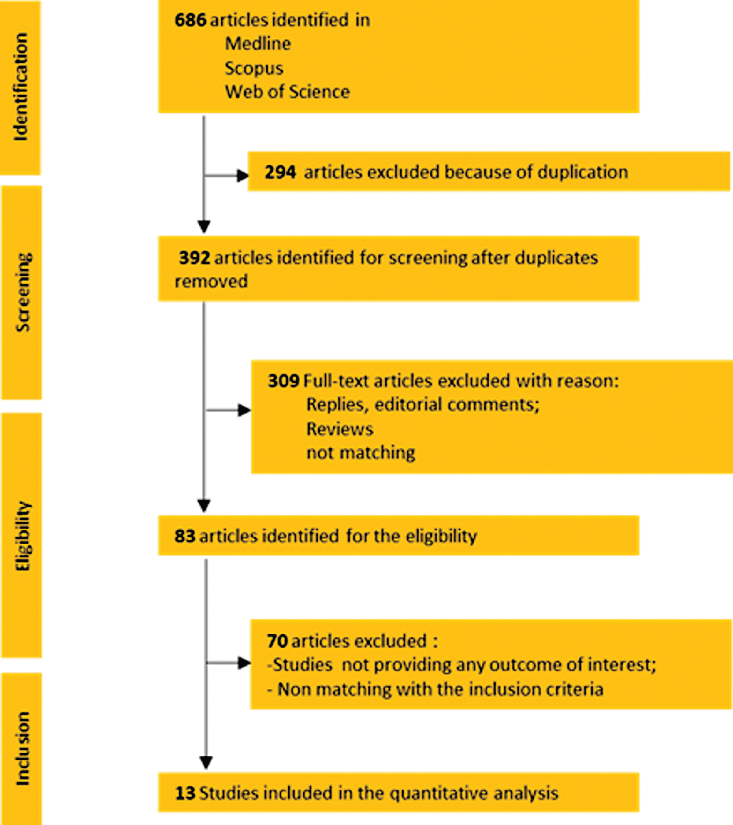
Of the 686 articles that were identified, 13 studies met the criteria for quantitative analysis. Staging, Grading and Tumor Classification, Prognosis, and Therapy Response were discussed in 7, 3, 2 and 7 studies, respectively. Data on cost of implementation were not reported. CT and MRI were the most common imaging approaches.
CONCLUSION:
Radiomics shows potential in bladder cancer detection, staging, grading, and response to therapy, thereby supporting the physician in personalizing patient management. Extension and validation of this promising technology in large multisite prospective trials is warranted to pave the way for its clinical translation.
INTRODUCTION
Bladder cancer is a potentially fatal disease associated with high rates of annual morbidity and mortality [1– 3]. The current strategy of clinical decision-making and follow-up management of bladder cancer is based on the reliable assessment of muscle invasion status, grade of malignancy, and pathology [4]. However, the observance of a high recurrence rate of 50– 80%, in the literature, in patients over the age of 65, highlights some of the limitations in these strategies, such as poor sensitivity (61%) for low-grade tumors, tumor heterogeneity-based sampling bias, and a complex interplay of molecular, histological and immune underpinnings in these tumors [3, 5– 7]. In addition to the difficulties in reliably detecting and characterizing tumor clinically, the prediction of treatment response is also a hurdle in the management of bladder cancer [8]. While new treatments are being administered to bladder cancer patients, a reliable method to predict the patient specific post-treatment response and thereby, decide between treatments is lacking. This conundrum creates a scenario where some patients receive ineffective therapies, with some treatments causing adverse reactions without an option to adjust treatment during the early stages of the disease.
Fig.1
Prisma Flowchart.
Radiomics is an emerging field of quantitative imaging with a variety of applications in clinical practice and research, particularly oncology. For oncologic applications, the technique potentially provides a comprehensive noninvasive characterization of the whole tumor, using a panel of quantifiable tumor metrics called the radiomics signature, extracted from multimodality medical images including computed tomography (CT), positron emission tomography (PET), magnetic resonance imaging (MRI), and ultrasonography (US) [9– 11]. While promising, radiomics is still novel to many radiologists and clinicians, and its clinical application is hampered by the limited availability of efficient and standardized systems of feature extraction and data sharing [12– 16]. Currently, the majority of the radiomics studies are retrospective, single institution studies with a relatively small sample size and thus statistically weak with poor generalization across different institutions. Larger studies conducted across multiple institutions are needed to validate these preliminary results [12].
Machine learning (ML) methods are designed to process large amounts of high-dimensional data, without a guiding (biomedical) hypothesis, to directly discover potentially actionable knowledge. Consequently, ML methods are increasingly being incorporated into radiomics studies, particularly for augmenting classification. While ML-augmented radiomics studies have demonstrated their utility for various purposes such as diagnosis, prognosis, and treatment response, the exploration has been limited and lacks rigor [17, 18]. For example, current ML-augmented radiomic approaches include the utilization of only a small number of classification methods, often of the same type (e.g. Support Vector Machine, Random Forest), the performance evaluation using the AUC score only, and the assessment of all possible combinations of radiomics and classification methods to identify the best possible classifier is non-systematic [19]. In this paper, we scope the current literature to systematically review promising applications and limitations of radiomics and ML-augmented radiomics in the management of bladder cancer.
EVIDENCE ACQUISITION
Search strategy
For the present systematic review, Pubmed ®, Scopus ®, and Web of Science ® databases were searched systematically for all full-text English-language articles assessing the impact of Artificial Intelligence OR Radiomics AND Bladder Cancer AND (staging OR grading OR prognosis) and published up to January 2020. References were manually reviewed to identify supplementary studies of interest. To ensure a transparent and thorough reporting of our findings, we followed the Preferred Reporting Items for Systematic Review and Meta-Analyses (PRISMA) statement.
Selection of eligible studies and data extraction
Two investigators (G.E.C and N.N.) independently screened all articles to identify studies that meet the inclusion criteria (Fig. 1). Any disagreements about eligibility were resolved by discussion between the two investigators until a consensus was reached. When an Institution published multiple papers with entirely overlapping surgical periods, only the latest published paper was considered. However, studies from the same institution with entirely or partially overlapping surgical periods but evaluating different study populations were included in the analysis.
All data retrieved from the systematically reviewed studies were recorded in an electronic database and the following outcomes were recorded: Number of Cases, Image Acquisition, Image Segmentation, Feature Extraction, Validation, and Outcomes of Interest (Staging, Grading, Tumor Classification, Prognosis and Therapy Response).
EVIDENCE SYNTHESIS
Of the 686 articles that were identified, 13 met the criteria for quantitative analysis (Fig. 1). Table 1 provides key details of these shortlisted studies, including year of publication, study design, number of patients evaluated, and imaging details. Data on cost were not reported. CT and MRI were the most common imaging approaches reported.
Radiomics workflow
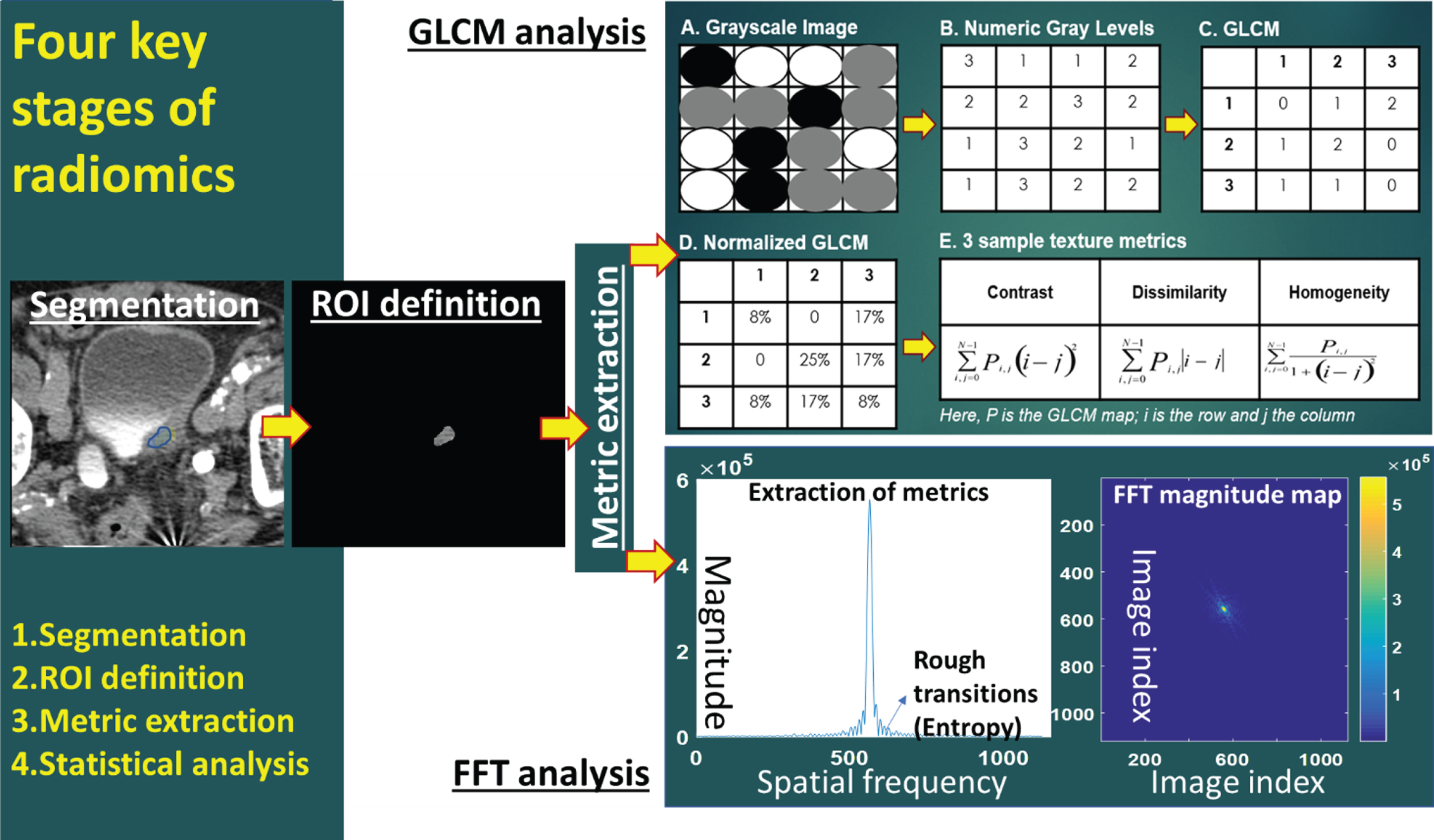
A typical radiomics workflow comprises 4 stages: image acquisition, image segmentation, feature extraction, and statistical analysis (Fig. 2, Table 1) [11]. Additional modules such as image registration, data formatting, de-noising etc. are used, however, they are modality- and application-specific. The reliable execution of each stage is critical to the success of the radiomics analysis, as each of these stages can be implemented distinctively across different studies (Table 1). Prior to undertaking any radiomics study, it is important to consider the quality and distribution of the data. Several guidelines have been reported in many studies [20– 22] to successfully design radiomic studies to overcome these pitfalls e.g. the radiomics quality score [23] and the TRIPOD (Transparent Reporting of a Multivariable Prediction Model for Individual Prognosis or Diagnosis) guidelines [24].
Table 1
Studies’ characteristics and radiomics workflow assessment
| Author | Year | Type of Study | Cases | Image Acquisition | Image Segmentation | Feature Extraction | Validation | Prediction Target |
| X.Xu [41] | 2019 | Retrospective | 71 | MRI (3T) - T2W, DW, ADC, and DCE | An axial image slice from MRI was selected based on largest tumor area and then two independent radiologists manually mapped a polygonal ROI to separate tumor from non-tumor and they agreed upon any discrepancies. ADC maps were then generated from DW images. | Features included 8 histogram, 39 CM, 33 RLM, 5 NGTDM, and 15 GLSZM. They were extracted using an online tool. | SVM-RFE was used to create a predictive model from the training cohort. LASSO was also used as a second option. It was used with the LIBSVM package with RBF on the validation cohort and performance data was collected. Validation cohort n = 21. | Two year recurrence risk |
| Wang [42] | 2019 | Retrospective | 100 | MRI (3T) - T2WI, DWI, and ADC | Two independent radiologists manually selected ROI slice by slice. Discrepancies were discussed. | All features were calculated for each slice and averaged within the 3D tumor volume using Pyradiomics. Features included: 14 shape-based features, 220 gray-level cooccurrence matrix (GLCM) features, 160 gray-level run length matrix (GLRLM) features, 160 gray-level size zone matrix (GLSZM) features, 50 neighborhood gray tone difference matrix (NGTDM) features, 140 neighboring gray-level dependence matrix (GLDM) features, and 180 first-order statistics features | Each feature subset was trained on a training cohort and tested on a validation cohort. Accuracy, sensitivity, specificity, and AUC values were tested. 2-Sample t test and LASSO selected features that were tested with multivariate logistic regression to test 5 models. | Pathologic grade of bladder tumor |
| Lin [43] | 2019 | Retrospective | 62 | CT | Tumor with largest diameter chosen with ITK-SNAP and single radiologist manually selected ROI | Ultrasonics software. 1076 imaging features were extracted from a single CT image, including a grey-level co-occurrence matrix, wavelet transform and local binary pattern and co-occurrence of the local anisotropic gradient orientation. | LASSO used to create model. No validation cohort. | Progression-free interval |
| S. Xu [44] | 2019 | Retrospective | 218 | MRI (3T) - DWI | One radiologist manually segmented the tumor via ITK-SNAP to reveal VOI. VOI was copied to ADC for computer analysis. A second radiologist confirmed a sample of the work. | Features were selected for intensity, texture, and shape. Texture was extracted from GLCM, GLRLM, GLSZM, and NGTDM. 156 features were extracted. | Random Forest (RAF) and Boruta used to create algorithms. Validation set consisted of 87 patients. | Muscle-invasive status of tumor |
| Cha 2016 [33] | 2016 | Retrospective | 62 | CT | One radiologist manually marked tumor locations in the scans and outlined the 3D contour with longest and perpendicular diameter measured with an institutionally-developed graphical interface. A second radiologist redid a sample of the work. | For each section, 16x16 pixel ROIs were extracted. | DL-CNN was used to create the algorithm. Its performance was then tested against the scans that had been manually marked. | Gross tumor volume |
| Cha 2017 [49] | 2017 | Retrospective | 123 | CT | 3-stage AI-CALS system was used. | ROIs of 16x32 pixels. | RAF-SL, RAF-ROI, and DL-CNN was used to create the algorithm. Their performance was then tested against a validation cohort of 41 pt. | Tumor response to chemotherapy |
| Garapati [45] | 2017 | Retrospective | 84 | CT | 3-stage AI-CALS system was used. | Five morphological features were extracted based on NRL. Texture features were obtained from RBST. A total of 91 features were extracted - 26 morphological and 65 textural. | LDA, NN, SVM, and RAF were compared against radiologist’s hand-segmented contours. | T stage greater than or equal to T2 or less than T2 |
| Zhang [46] | 2017 | Retrospective | 61 | MRI (3T) - DWI and ADC | 3D VOIs were generated by stacking 2D ROIs from DW images. All images were reviewed by two independent radiologists who discussed any discrepancies. | 9 histogram features and 42 GLCM features were derived from each image - a total of 102 features were extracted from both DWI and ADC maps | SVM-RFE was used to generate the algorithm. LIBSVM was used to create 5 feature sets to test between high and low grade tumors. The optimized classifier was tested with 100 rounds of 10-fold cross-validation randomly to demonstrate its generalization and stability. | Tumor grade |
| Zheng [47] | 2019 | Retrospective | 199 | MRI | Whole tumor besides base was segmented. VOIs were semiautomatically generated using “3D Slicer.”; | 1301 features were extracted from two VOIs using “3D Slicer” | LASSO used to create the algorithm. It was then tested on the validation cohort of 69. | Muscle-invasive status of tumor |
| Fan [50] | 2018 | Retrospective - database | 33 | CT | A fellowship-trained radiologist manually identified regions of interest for UCs and MPCs. | MATLAB code was used to extract voxel data | 2D CTTA was performed on an area of the tumor with the largest diameter using pre-segmented tumor images and histogram analysis, GLCM, GLDM, and FTT were compared between the radiologist and CTTA group. | Urothelial vs. micropapillary tumors |
| Lim [51] | 2018 | Retrospective | 36 | MRI (3T and 1.5T) -T2 and ADC | Two fellowship-trained radiologists identified the dominant tumor location. | TexRAD was used to extract textural features. | No comparison between a computer-derived identification and human-derived. This paper focuses on texture features between different stages of tumor. | Tumor stage |
| Alessandrino [52] | 2019 | Retrospective | 42 | CT | Two fellowship-trained radiologists outlined lesions manually. | TexRAD was used to extract textural features. | Textures were analyzed via histogram technique and included mean, SD, entropy, MPP, skewness, and kurtosis. There was no validation cohort. A predictive model was developed to show which features correlated best with PFS. | Metastatic urothelial carcinoma response to programmed death-ligand 1 inhibitors |
Studies characteristics. MRI: Magnetic Resonance Imaging; T2W: T2-weighted; DW: diffusion-weighted; ADC apparent diffusion coefficient; DCE dynamic contrast-enhanced; 3T: 3 Tesla; ROI: Region of interest; AI-CALS Auto-initialized cascaded level set; VOI: Volumes of interest; LASSO: least absolute shrinkage and selection operator; GLCM: Gray Level Co-occurrence Matrix; GLSZM, Gray Level Size Zone Matrix; NGTDM: Neighboring Gray Tone Difference Matrix; SVM-RFE: support vector machine with recursive feature elimination; DL-CNN: deep Learning convolutional neura l network; LDA: Linear Discriminant Analysis; NN: nearest neighbor; SVM: support vector machine; RAF: Random forest; SVM-RFE: support vector machine with recursive feature elimination; CTTA: Computed tomography texture analysis; FTT: Fast Fourier Transform SSF: spatial scale filters; MPP: Mean positive pixel.
Fig.2
Workflow of radiomics (ROI = region of interest; GLCM = gray level co-occurrence matrix; FFT = fast Fourier transform).
Multiple studies have shown that radiomic feature values are sensitive to the acquisition and reconstruction parameters, thus hindering the pooling of data and comparing the results acquired using different scanners or protocols [13]. Physical phantoms have been used in quantitative imaging to explore and quantify sources of bias and variance for e.g. initiatives by the Radiological Society of North America (RSNA) Quantitative Imaging Biomarker Alliance (QIBA) [25], the Credence Cartridge Radiomics phantom [16] etc. In some cases, virtual phantoms, or digital reference objects (DROs) have also been useful for evaluation of software packages that are used to derive quantitative imaging biomarkers. By providing a dataset and a set of metric evaluation that can be accessed by all, radiomics can be rigorously tested in large multi-institution studies to aid its clinical translation. One such major effort is the Image Biomarker Standardization Initiative (IBSI) that aims to standardize radiomics imaging biomarkers [26].
While in some case these calibration objects have been used for standardization of imaging data acquired using diverse scanner, scanning and post processing protocols [15, 27], others use the same approach to identify radiomic metrics that are reliable [14] (robust, repeatable and reproducible) to facilitate big data radiomics using data pooled from reliable radiomic metrics acquired from multiple institutions.
Image acquisition
This is the first step of the radiomics workflow, and the end-product of this step is an image volume (if 3D) or image cross-section (if 2D) stored in the Picture Archiving and Communication System (PACS), typically in a Digital Imaging and Communication in Medicine (DICOM) format. Currently, different imaging centers follow distinct image acquisition protocols to ensure the quality of imaging set up by their respective institutions [12, 14, 16]. The lack of consensus or guidelines on image acquisition across institutions leads to imaging data heterogeneity among different radiomics studies. This issue is further compounded by a lack of thorough and consistent labeling, annotation, segmentation, and quality assurance within the routine clinical workflow. Even in centers that do the additional steps, there is no consensus on the process. In general, considering the hardware and software variables that can vary across the different imaging modalities (CT, MRI, PET, and US), overcoming the issue of data heterogeneity is a complex task. One path adopted to overcome the effects of data heterogeneity on radiomics is data preprocessing to ensure consistency and comparability [15, 27]. Data preprocessing steps include but not limited to steps for standardizing imaging protocols preacquisition [15] or harmonizing data post acquisition [20]. While the solution is promising, it is not readily scalable, as newer and better imaging technologies are always evolving, preventing a comprehensive assessment of the heterogeneity. The second approach to overcome the effects of data heterogeneity on radiomics is to conduct comprehensive imaging experiments using phantoms (standardization objects) to identify radiomic metrics that are reliable [14, 16, 28– 31]. Reliable radiomic metrics are reproducible, robust, and repeatable across multicenter studies [14]. While the performance of the latter approach is dependent on the reliability and suitability of the phantom to the clinical question, the approach can conceivably find reliable radiomics signatures for use in multicenter studies without the need for an additional pre-processing step.
Image segmentation
This is the second step of the radiomics workflow, and the end-product of this step is the isolation of a region of interest (ROI), which can be either a volume (if 3D) or an area (if 2D). While it is intuitive to expect 3D radiomics to outperform 2D radiomics, this is not always the case [32]. As in the case of image acquisition, there are no established guidelines or consensus across centers with regards to image segmentation. While some centers perform manual segmentation to gain accuracy in lieu of efficiency, others perform automated segmentation (e.g. seed growing method). While automated segmentation promotes consistency and workflow optimization, it is difficult to establish a segmentation criteria for bladder cancers, considering the sometimes indistinct borders of tumors, marked variability of bladder distensibility, and inconsistent tumor imaging appearances [33]. Moreover, while manual segmentation is easy to implement, it is tedious, time consuming and subject to intra- and inter-observer measurement variability [34] leading to difficulties in radiomic feature reproducibility. Semi-automation has been investigated, and may provide a middle ground regarding the issue of segmentation [35]. Tumor microenvironment may provide valuable information [36], however, there is no consensus about what should be included in the segmented ROI.
Feature extraction
This is the third step of the radiomics workflow, and the end-product of this step is a feature map comprising of a number of metrics extracted from the segmented ROI, using a variety of feature extraction techniques implemented using a sophisticated suite of data characterization algorithms. The commonly used features within a radiomics framework include texture, shape, and size metrics [9– 11]. Texture features can be classified into first-order statistical features, second-order statistical features, and higher-order statistical features, depending on if the intensity values are used only, or if both the intensity values and their orientation within the ROI are used together [37, 38]. Higher-order statistical features are the products of mathematical transformations such as wavelets, Minkowski function etc., which have the capability of decomposing the images into multiple levels of information (scales) to conduct a more in-depth analysis.
While the fundamental mathematical principles behind the texture techniques and metrics are the same, the implementation is different across different centers [39, 40]. Even the number of texture metrics used within a radiomics panel varies drastically across different studies. These variabilities in conducting radiomic studies, in the absence of established guidelines or consensus, have led to scenarios where the results are non-reproducible and non-comparable.
Radiomics and bladder cancer tumor staging
Seven radiomic studies in our list evaluated tumor stage as a clinical characteristic in bladder cancer. Xu et al. [41] evaluated patients with both non-muscle invasive disease (NMIBC) (T1 or lower) or muscle invasive bladder cancer (MIBC) (T2 or higher) who underwent either transurethral resection of bladder tumor or radical cystectomy. Muscle invasive status was associated with a 2.2-fold increased risk of disease recurrence on multivariable analysis. Wang et al. [42] used pre-operative radiomic analysis to estimate pathological grade in patients with Tis-T3 disease. 24.3% and 16.7% of patients had MIBC in training and validation sets. The remainder had NMIBC. Lin et al. [43] used a combination of clinicopathologic data, gene expression profiles, and CT-based radiomic studies to evaluate survival in 62 patients with bladder cancer. 67.7% of their patients had NMIBC compared to 32.3% with muscle-invasive disease. They were the only study to comment on the observance of lymphatic involvement. 30.6% of patients had clinical N1-3 disease. Xu et al. [44] reported on the incorporation of diffusion weighted magnetic resonance imaging alongside traditional clinical staging in order to more accurately identify muscle invasive disease status. 60% of patients had NMIBC and the remaining 40% had MIBC. Garapati et al. [45] utilized computed tomographic delayed phase imaging to predict muscle invasive disease status in 84 tumors from 76 patients. 52% had non-muscle invasive disease (< /=T1) versus 48% with muscle invasion (> /=T2). Zhang et al. [46] also evaluated NMIBC vs. MIBC as a baseline clinical characteristic in 61 patients. NMIBC was reported in 28 patients, and MIBC in 27 patients; the remainder had missing stage status. Lastly, Zheng et al. [47] pre-operatively evaluated muscle invasiveness using an MRI-based radiomic signature. MRI-determined clinical staging demonstrated MIBC in 63.1% and 60.9% of training and validation sets. Pathological staging demonstrated MIBC in 43.1 and 44.9% of training and validation sets.
Radiomics and bladder cancer tumor grading
Tumor grade was reported in three radiomics studies in bladder cancer [41, 42, 46]. Xu et al. had 36.6% of patients with low-grade disease and 63.4% with high-grade disease [41]. Tumor grade was not a significant predictor of recurrence in multivariable analysis. Wang et al. had 56 patients with low-grade and 44 patients with high-grade disease [42]. Zhang et al. had 32 patients with low-grade disease and 29 patients with high-grade bladder cancer [46].
Prognosis and response to therapy
Twelve papers reported therapeutic responses in bladder cancer based on radiomics predictions (Table 1). Xu et al. created a nomogram to predict tumor recurrence within two years of TURBT or RC based on both radiomic and clinical factors [41]. Radiomics features were gathered from MRI images using T2W, DW, and DCE image sequences [41]. The authors used SVM-RFE and LASSO algorithms to extract the most predictive image features. Thirty-two image features were found to generate the highest area under the curve value for the “radiomics score” in predicting bladder cancer recurrence [41]. Xu et al. reported that the radiomics score had a 8.2 odds ratio effect on prognosis with a 2.4– 27.8 95% confidence interval [41]. Radiomics had a significant effect on prognosis with a p-value < <0.05 [33]. In the validation cohort, the sensitivity of the radiomics features based on the SVM-RFE and Lasso algorithms was 77.8% and 55.6%, respectively [41]. The specificity of the radiomics features based on the SVM-RFE and Lasso algorithms was 73.8% and 75%, respectively [41]. The accuracy of the radiomics features based on the SVM-RFE and Lasso algorithms was 75.5% and 66.7%, respectively, and adjusted to 80.1% after risk stratification [41]. Similarly, the area under the curve for SVM-RFE selected features was 0.82 and 0.72 for Lasso with a correction to 0.84 after risk stratification [41]. MRI image features derived from both SVM-RFE and Lasso algorithms predicted bladder cancer recurrence within two years in the validation cohort with a p-value < <0.01 for SVM-RFE and <0.05 for LASSO [41].
Wang et al. developed a radiomics model based on MRI images to predict pathological grade of bladder tumors [42]. They did not evaluate prognostic factors, such as overall survival or time to recurrence [42]. Their radiomics models were derived from the following imaging modalities: T2-weighted imaging (T2WI; diffusion-weighted imaging (DWI); apparent diffusion coefficient maps (ADC), and modeling modalities: Max-out Model and Joint Model [42]. Regarding sensitivity, T2WI was 76.9%, DWI was 76.9%, ADC was 84.6%, Max-out was 76.9%, and joint was 76.9% [42]. The specificity for T2WI was 76.4%, DWI was 76.4%, ADC was 76.4%, Max-out was 88.2%, and joint was 83.3% [42]. Accuracy for T2WI was 76.7%, DWI was 76.7%, ADC was 80%, Max-out was 83.3%, and joint was 83.3% [42]. Area under the curve testing the ability of the models to predict pathologic grade for T2WI was 0.782, DWI was 0.769, ADC was 0.805, Max-out was 0.919 and joint was 0.928 [42].
Lin et al. created a nomogram based on radiomics features derived from contrast-enhanced CT images, transcriptomics, and clinical features to sort patients into low or high risk groups for progression-free interval [43]. In multivariate analysis, Lin et al. reported a hazard ratio of 1.99 (1.015– 3.912) in predicting progression-free interval based on radiomics alone and 2.588 (1.317– 5.085) based on transcriptomics [43]. In their multivariate analysis, they reported an area under the curve for radiomics of 0.956 versus 0.948 for transcriptomics [43]. These findings were significant with a p value of 0.045 for radiomics and 0.006 for transcriptomics [43].
Xu et al. investigated the ability of their Random Forest (RF) radiomics algorithm based on DWI sequence MRI image features to predict the muscle-invasive status of bladder tumors [44]. Xu et al. reported that their radiomics model was more sensitive than TUR and qualitative MRI analysis for discriminating muscle-invasive disease [44]. They reported a sensitivity of 87.3% for their RF model vs. 65.5% for TUR alone and 76.4% for qualitative MRI alone [44]. RF and TUR combined led to a sensitivity of 96.4% [44]. The specificity of RF was reported at 78.1% and the accuracy of RF alone was 83.9% [44]. The accuracy of the combined RF radiomics model and TUR data was 89.7%. The area under the curve for RF alone in predicting muscle invasion was 0.907 [44].
Suarez-Ibarrola et al. is a literature review that reported prognostic predictions, including recurrence and survival, from several studies [48]. Details can be found in Table 2. Cha et al. 2016 tested the ability of their radiomics model to accurately measure the change in gross tumor volume in preoperative and postoperative CT scans [33]. They reported an area under the curve of 0.73±0.6 for the deep-learning convolution neural network (DL-CNN) model and 0.70±0.07 for the auto-initialized cascaded level sets model [33]. Both of these models out-performed the radiologists (Table 2) [33].
Table 2
Outcomes of interest: prediction target.
| Author | Stage | Grade | Prognosis | Therapy Response | |||||||||
| OR | Hazard Ratio | 95% CI | P-value | Notes | Sensitivity (%) | Specificity (%) | Accuracy (%) | AUC | 95% CI | P-value | |||
| X. Xu [41] | Training: | NMIBC Recurrent: 7 (14%) | Low Recurrent: 8 (16%) | MIS: 2.166 | MIS: 1.154– 4.066 | MIS:<0.05 | Both MIS and Rad-Score were independent predictors of recurrence. | SVM-RFE: 84.00 | SVM-RFE: 80.00 | SVM-RFE: 82.00 | SVM-RFE: 0.8593 | SVM-RFE: (0.8425– 0.8810) | SVM-RFE:< <0.01 |
| NMIBC Nonrecurrent: 15 (30%) | Low Nonrecurrent: 9 (18%) | Rad-Score: 8.191 | Rad-Score: 2.415– 27.780 | Rad-Score:< <0.05 | Lasso: 73.74 | Lasso: 71.08 | Lasso: 72.41 | Lasso: 0.7504 | Lasso: (0.7364– 07613) | Lasso:<0.05 | |||
| MIBC Recurrent: 18 (36%) | High Recurrent: 17 (34%) | After risk stratification: 88 | After risk stratification: 0.915 | ||||||||||
| MIBC Nonrecurrent: 10 (20%) | High Nonrecurrent: 16 (32%) | ||||||||||||
| Validation: | NMIBC Recurrent: 6 (28.57%) | Low Recurrent: 4 (19.05%) | SVM-RFE: 77.78 | SVM-RFE: 73.83 | SVM-RFE: 75.52 | SVM-RFE: 0.8216 | SVM-RFE: (0.8130– 0.8301) | SVM-RFE:< <0.01 | |||||
| NMIBC Nonrecurrent: 8 (38.10%) | Low Nonrecurrent: 5 (23.81%) | Lasso: 55.566 | Lasso: 75.00 | Lasso: 66.67 | Lasso: 0.7222 | Lasso: (0.7003– 0.7328) | Lasso:<0.05 | ||||||
| MIBC Recurrent: 3 (14.29%) | High Recurrent: 5 (23.81%) | After risk stratification: 80.95 | After risk stratification: 0.838 | ||||||||||
| MIBC Nonrecurrent: 4 (19.05%) | High Nonrecurrent: 7 (33.33%) | ||||||||||||
| Total: | NMIBC: 36 (50.7%) | LOW: 26 (36.6%) | |||||||||||
| MIBC: 35 (49.3% | HIGH: 45 (63.4%) | ||||||||||||
| Wang [42] | Training: | LOW: 39/70 (53.01%) | T2WI: 0.7467 (0.6764– 0.8170) | T2WI: 0.7967 (0.7438– 0.8495) | T2WI: 0.7743 (0.7311– 0.8174) | T2WI: 0.7933 (0.7471– 0.8396) | |||||||
| HIGH: 31/70 (46.99%) | DWI: 0.7067 (0.6321– 0.7812) | DWI: 0.7400 (0.6847– 0.7953) | DWI: 0.7257 (0.6710– 0.7805) | DWI: 0.8083 (0.7565– 0.8601) | |||||||||
| ADC: 0.8100 (0.7335– 0.8865) | ADC: 0.8250 (0.7767– 0.8733) | ADC: 0.8171 (0.7779– 0.8564) | ADC: 0.8350 (0.7924– 0.8776) | ||||||||||
| Max-out: 0.8283 (0.7533– 0.9034) | Max-out: 0.8533 (0.8004– 0.9062 | Max-out: 0.8429 (0.7967– 0.8890) | Max-out: 0.8850 (0.8413– 0.9287) | ||||||||||
| Joint: 0.8267 (0.7609– 0.8925) | Joint: 0.8783 (0.8330– 0.9236) | Joint: 0.8543 (0.8181– 0.8905) | Joint: 0.9233 (0.9001– 0.9466) | ||||||||||
| Validation: | LOW: 17/30 (53.12%) | T2WI: 0.7692 | T2WI: 0.7647 | T2WI: 0.7667 | T2WI: 0.7828 | ||||||||
| HIGH: 13/30 (46.88%) | DWI: 0.7692 | DWI: 0.7647 | DWI: 0.7667 | DWI: 0.7692 | |||||||||
| ADC: 0.8462 | ADC: 0.7647 | ADC: 0.8000 | ADC: 0.8054 | ||||||||||
| Max-out: 0.7692 | Max-out: 0.8824 | Max-out: 0.8333 | Max-out: 0.9186 | ||||||||||
| Joint: 0.7692 | Joint: 0.8824 | Joint: 0.8333 | Joint: 0.9276 | ||||||||||
| Total: | TIS: 1, Ta: 9, T1 : 68, T2 : 17, and T3 : 5 | LOW: 56, TOTAL HIGH: 44 | |||||||||||
| Lin [43] | AJCC I: 0 AJCC II: 22 AJCC III: 21 AJCC IV: 19 | Radiomics: 1.993 (1.015– 3.912) | Multivariate | Radiomics: 0.045 | |||||||||
| T1 : 4 T2 : 38 T3 : 17 T4 : 3 | Transcriptomics: 2.588 (1.317– 5.085) | Radiomics: 0.956 | Transcriptomics: 0.006 | ||||||||||
| N0 : 35 N1-3 : 19 NA: 8 | Transcriptomics: 0.948 | ||||||||||||
| S. Xu [44] | Training: | Clinically NMIBC: 80 | |||||||||||
| Clinically MIBC: 51 | |||||||||||||
| Pathologically NMIBC: 45 | |||||||||||||
| Pathologically MIBC: 86 | |||||||||||||
| Validation: | Clinically NMIBC: 51 | ||||||||||||
| Clinically MIBC: 36 | |||||||||||||
| Pathologically NMIBC: 32 | |||||||||||||
| Pathologically MIBC: 55 | |||||||||||||
| Total: | Clinically NMIBC: 131 | RandomForest model was more sensitive than TUR and MRI for discriminating MIBC | RF: 0.873 (vs TUR at 0.655 and MRI at 0.764) | RF: 0.781 | RF: 0.839 | RF: 0.907 | |||||||
| Clinically MIBC: 87 | RF+TUR: 0.964 | RF+TUR: 0.897 | |||||||||||
| Pathologically NMIBC: 77 | |||||||||||||
| Pathologically MIBC: 141 | |||||||||||||
| Suarez-Ibarrola [48] | >70% for recurrence and survival at 1, 3, and 5 years (Hasnain) | >70% for recurrence and survival at 1, 3, and 5 years (Hasnain) | 83% low vs high grade (Zhang) | 0.90 (Xu) | |||||||||
| 0.90 (Xu) | 0.85 (Xu) | 94% when combined with atomic force microscopy (Sokolov) | 0.86 (Zhang) | ||||||||||
| 0.78 (Zhang) | 0.87 (Zhang) | 0.88 (Xu) | 0.76– 0.77 (Wu) | ||||||||||
| 0.83 (Zhang) | 0.80 for CDSS alone, 0.74 for no CDSS, and 0.77 for physicians and CDSS (Cha) | ||||||||||||
| Cha 2016 [33] | Volume | ||||||||||||
| DL-CNN: 0.73+/– 0.06 | |||||||||||||
| AI-CALS: 0.70+/– 0.07 | |||||||||||||
| Radiologist: 0.70+/– 0.06 | |||||||||||||
| WHO criteria | |||||||||||||
| Rad1 : 0.63+/–.07 | |||||||||||||
| Rad2 : 0.61+/–.06 | |||||||||||||
| RECIST | |||||||||||||
| Rad1 : 0.65+/–.07 | |||||||||||||
| Rad2 : 0.63+/–.06 | |||||||||||||
| Cha 2017 [49] | DL-CNN: 6 (50%) | DL-CNN: 34 (81%) | DL-CNN: 0.73+/– 0.08 | ||||||||||
| RF-SL: 6 (50%) | RF-SL: 33 (78.6%) | RF-SL: 0.77+/– 0.08 | |||||||||||
| RF-ROI: 8 (66.7%) | RF-ROI: 23 (54.8%) | RF-ROI: 0.69+/– 0.08 | |||||||||||
| Rad1 : 11 (91.7%) | Rad1 : 18 (42.9%) | Rad1 : 0.76+/– 0.08 | |||||||||||
| Rad2 : 11 (91.7%) | Rad2 : 16 (38.1%) | Rad2 : 0.77+/– 0.07 | |||||||||||
| Garapat [45] i | Training: | <T2 : 43 (not treated | LDA Morph Set 1 : 0.91 | ||||||||||
| with | LDA Morph Set 2 : 0.97 | ||||||||||||
| NAC)≥T2 : 41(treated | LDA Text Set 1 : 0.91 | ||||||||||||
| with NAC) | LDA Text Set 2 : 1. | ||||||||||||
| LDA Comb Set 1 : 0.92 | |||||||||||||
| LDA Comb Set 2 : 1 | |||||||||||||
| NN Morph Set 1 : 0.96 | |||||||||||||
| NN Morph Set 2 : 0.98 | |||||||||||||
| NN Text Set 1 : 0.95 | |||||||||||||
| NN Text Set 2 : 1 | |||||||||||||
| NN Comb Set 1 : 0.97 | |||||||||||||
| NN Comb Set 2 : 1 | |||||||||||||
| SVM Morph Set 1 : 0.95 | |||||||||||||
| SVM Morph Set 2 : 0.97 | |||||||||||||
| SVM Text Set 1 : 0.92 | |||||||||||||
| SVM Text Set 2 : 1 | |||||||||||||
| SVM Comb Set 1 : 0.92 | |||||||||||||
| SVM Comb Set 2 : 1 | |||||||||||||
| RAF Morph Set 1 : 1 | |||||||||||||
| RAF Morph Set 2 : 1 | |||||||||||||
| RAF Text Set 1 : 1 | |||||||||||||
| RAF Text Set 2 : 1 | |||||||||||||
| RAF Comb Set 1 : 1 | |||||||||||||
| RAF Comb Set 2 : 1 | |||||||||||||
| Validation: | LDA Morph Set 1 : 0.90 | ||||||||||||
| LDA Morph Set 2 : 0.81 | |||||||||||||
| LDA Text Set 1 : 0.91 | |||||||||||||
| LDA Text Set 2 : 0.88 | |||||||||||||
| LDA Comb Set 1 : 0.89 | |||||||||||||
| LDA Comb Set 2 : 0.90 | |||||||||||||
| NN Morph Set 1 : 0.88 | |||||||||||||
| NN Morph Set 2 : 0.91 | |||||||||||||
| NN Text Set 1 : 0.89 | |||||||||||||
| NN Text Set 2 : 0.92 | |||||||||||||
| NN Comb Set 1 : 0.91 | |||||||||||||
| NN Comb Set 2 : 0.95 | |||||||||||||
| SVM Morph Set 1 : 0.88 | |||||||||||||
| SVM Morph Set 2 : 0.90 | |||||||||||||
| SVM Text Set 1 : 0.91 | |||||||||||||
| SVM Text Set 2 : 0.89 | |||||||||||||
| SVM Comb Set 1 : 0.92 | |||||||||||||
| SVM Comb Set 2 : 0.89 | |||||||||||||
| RAF Morph Set 1 : 0.83 | |||||||||||||
| RAF Morph Set 2 : 0.88 | |||||||||||||
| RAF Text Set 1 : 0.89 | |||||||||||||
| RAF Text Set 2 : 0.97 | |||||||||||||
| RAF Comb Set 1 : 0.86 | |||||||||||||
| RAF Comb Set 2 : 0.96 | |||||||||||||
| Zhang [46] | NMIBC and low grade: 19 (59.4%) | LOW: 32 | 23 (78.4%) | 28 (87.1%) | 51 (82.9%) | 0.861 | 0.851– 0.870 | <0.01 | |||||
| NMIBC and high grade: 9 (31.0%) | HIGH: 29 | ||||||||||||
| MIBC and low grade: 9 (28.1%) | |||||||||||||
| MIBC and high grade: 18 (62.1%) | |||||||||||||
| Zheng [47] | Training: | Clinically<cT2 : 48 (36.9%) | Radiomics | ||||||||||
| Clinically≥cT2 : 82 (63.1%) | 0.913 (0.864– 0.963) | ||||||||||||
| Pathologically<pT2 : 74 (56.9%) | optimism-corrected AUC: 0.912 | ||||||||||||
| Pathologically≥pT2 : 56 (43.1%) | Nomogram | ||||||||||||
| 0.922 (0.879– 0.965) | |||||||||||||
| optimism-corrected AUC: 0.921 | |||||||||||||
| Validation: | Clinically<cT2 : 27 (39.1%) | Discriminatory accuracy for T stage: 0.919 (.882–.956) compared to TURBT at 0.803 (.750–.858) | Radiomics | ||||||||||
| Clinically≥cT2 : 42 (60.9%) | 0.874 (0.791– 0.958) | ||||||||||||
| Pathologically<pT2 : 38 (55.1%) | Nomogram | ||||||||||||
| Pathologically≥pT2 : 31 (44.9%) | 0.876 (0.791– 0.961) | ||||||||||||
| Fan [50] | Muslce invasive UCs: 14 (42.4%) | ||||||||||||
| Muscle invasive MPCs: 31 (93.9%) | |||||||||||||
| Lim [51] | ≤T2 vs.≥T3 | ≥T2 : 26 (72.2%)≥T3 : 19 (52.8%) | Tumor | Tumor | Univariate | Tumor | |||||||
| ≥T3 vs.≤T2 T2 entropy: 4.56 | ≥T3 vs.≤T2 T2 entropy: 1.49– 20.41 | Tumor | ≥T3 vs.≤T2 T2 entropy: 0.85 | ||||||||||
| ≥T3 vs.≤T2 ADC entropy: 2.24 | ≥T3 vs.≤T2 ADC entropy: 1.13– 5.31 | ≥T3 vs.≤T2 T2 entropy: 0.004 | ≥T3 vs.≤T2 ADC entropy: 0.80 | ||||||||||
| Extravesical Fat | Extravesical Fat | ≥T3 vs.≤T2 T2 kurtosis: 0.018 | Extravesical Fat | ||||||||||
| ≥T3 vs.≤T2 T2 entropy: 17.50 | ≥T3 vs.≤T2 T2 entropy: 3.01– 200.80 | ≥T3 vs.≤T2 ADC entropy: 0.002 | ≥T3 vs.≤T2 T2 entropy: 0.84 | ||||||||||
| ≥T3 vs.≤T2 ADC entropy: 6.54 | ≥T3 vs.≤T2 ADC entropy: 1.90– 32.40 | ≥T3 vs.≤T2 T2 kurtosis: 0.011 | ≥T3 vs.≤T2 ADC entropy: 0.82 | ||||||||||
| Extravesical Fat | |||||||||||||
| ≥T3 vs.≤T2 T2 entropy: 0.001 | |||||||||||||
| ≥T3 vs.≤T2 ADC entropy: 0.001 | |||||||||||||
| Multivariate | |||||||||||||
| Tumor | |||||||||||||
| ≥T3 vs.≤T2 T2 entropy: 0.006 | |||||||||||||
| ≥T3 vs.≤T2 ADC entropy: 0.019 | |||||||||||||
| Extravesical Fat | |||||||||||||
| ≥T3 vs.≤T2 T2 entropy: 0.005 | |||||||||||||
| ≥T3 vs.≤T2 ADC entropy: 0.002 | |||||||||||||
| T1 vs.≥T2 | Tumor | Tumor | Univariate | Tumor | |||||||||
| ≥T3 vs.≤T2 ADC entropy: 2.11 | ≥T3 vs.≤T2 ADC entropy: 1.08– 5.03 | Tumor | ≥T3 vs.≤T2 ADC entropy: 0.76 | ||||||||||
| Extravesical Fat | Extravesical Fat | ≥T3 vs.≤T2 T2 entropy: 0.016 | Extravesical Fat | ||||||||||
| ≥T3 vs.≤T2 ADC entropy: 3.8 | ≥T3 vs.≤T2 ADC entropy: 1.25– 16.97 | ≥T3 vs.≤T2 ADC entropy: 0.019 | ≥T3 vs.≤T2 T2 entropy: 0.78 | ||||||||||
| Extravesical Fat | ≥T3 vs.≤T2 ADC entropy: 0.74 | ||||||||||||
| ≥T3 vs.≤T2 T2 entropy: 0.010 | |||||||||||||
| ≥T3 vs.≤T2 ADC entropy: 0.029 | |||||||||||||
| Multivariate | |||||||||||||
| Tumor | |||||||||||||
| ≥T3 vs.≤T2 ADC entropy: 0.027 | |||||||||||||
| Extravesical Fat | |||||||||||||
| ≥T3 vs.≤T2 ADC entropy: 0.010 | |||||||||||||
| Alessandrino [52] | Metastatic urothelial carcinoma: 42 (100%) | Predicting PFS: | Predicting PFS: | Predicting PFS: | Predicting PFS: | Predicting PFS: | Predicting PFS: | ||||||
| Entropy 45.49 | Entropy (2.25– 7156.46) | Entropy 0.044 | Entropy 58% | Entropy 90% | Entropy 69% | ||||||||
| Mean 1.09 | Mean (1.02– 1.23) | Mean 0.042 | Mean 53% | Mean 90% | Mean 65% | ||||||||
| Combined model < 0.0007 | Combined model 95% | Combined model 80% | Combined model 90% | ||||||||||
Cha et al. 2017 created a radiomics model based on pretreatment and post-treatment CT scans to identify complete vs. incomplete tumor response to chemotherapy [49]. They compared the following models: deep-learning convolution neural network (DL-CNN); radiomics feature based approach (RF-SL), and radiomics features from image patterns (RF-ROI) [49]. DL-CNN achieved a sensitivity of 50% and a specificity of 81%, RF-SL achieved a sensitivity of 50% and specificity of 78.6%, and ROI achieved a sensitivity of 66.7% and specificity of 54.8% [49]. The radiologists compared against had higher sensitivities and lower specificities (Table 2). The area under the curve for predicting chemotherapy treatment response for DL-CNN was 0.73±0.08, RF-SL was 0.77±0.08, and ROI was 0.69±0.08 [49]. These were similar to the area under the curve scores from the radiologist reads (Table 2).
Garapati et al. reported the area under the curve showing the ability of several algorithms based on radiomics features to stage tumors as greater than or less than T2 based on CT urography [45]. They included linear discriminant analysis (LDA), neural network (NN), support vector machine (SVM), and Radom Forest (RAF) models in their analysis with various sub analyses based on texture features (text), morphology features (morph), and combined features (comb) [45]. The area under the curve for all the models in the validation cohort ranged from 0.81– 0.97 [45]. A detailed breakdown can be found in Table 2.
Zhang et al. created a radiomics model based on texture features from DWI sequence MRI images to predict grade of bladder tumor [46]. They reported a sensitivity of 78.4%, specificity of 87.1%, and accuracy of 82.9% based on their model [46]. They found an area under the curve for the ability of their radiomics model to predict tumor grade of 0.861 [46]. Their findings were significant with a confidence interval of 0.851– 0.870 and a p-value of <0.01 [46].
Zheng et al. also created a nomogram to predict muscle invasive vs. non-muscle invasive tumors based on combined radiomics and clinical data [47]. Radiomics features were extracted from T2-weighted MRI images and the LASSO algorithm was used to select the most predictive features [47]. Zheng et al. compared the accuracy of their nomogram to TURBT and found the accuracy of the model was 91.9% (88.2– 95.6%) while the accuracy of TURBT was 80.3% (75.0– 85.8%) [47]. The area under the curve for the nomogram was 0.921. The area under the curve for the radiomics model alone in predicting muscle-invasion was 0.874 (0.791– 0.958) [47].
Fan et al. reported on the ability of CT based texture analysis to distinguish between urothelial carcinomas of the bladder and micropapillary carcinomas of the badder [50]. They found that 28/58 texture metrics were significantly different between urothelial and micropapillary tumors and 27/58 texture metrics were significantly different in the peritumoral fat surrounding urothelial vs. micropapillary tumors [50]. Further details can be found in Table 2. Lim et al. used texture features from T2-weighted and ADC MRI images to extract entropy values in tumor and extravesical fat to predict ≤T2 vs. ≥T3 and T1 vs. ≥T2 disease in tumor and fat, respectively [51]. In the ≤T2 vs. ≥T3 tumor group, T2 entropy was reported to have an odds ratio of 4.56 and ADC entropy an odds ratio of 2.24. In the ≤T2 vs. ≥T3 extravesical fat group, T2 entropy was associated with an odds ratio of 17.50 and ADC entropy with an odds ratio of 6.54 [51]. In the T1 vs. ≥T2 group, ADC entropy in the tumor region resulted in an odds ratio of 2.11 and in the extravesical fat bed, an odds ratio of 3.8 [51]. These findings were significant (Table 2). The area under the curve for the ≤T2 vs. ≥T3 tumor region with T2 entropy was 0.85 and with ADC entropy was 0.80 [51]. In the extravesical, T2 entropy resulted in an under the curve of 0.84 and ADC entropy in an area under the curve of 0.82 [51]. In the T1 vs. ≥T2 tumor group, area under the curve for ADC entropy was 0.76 [51]. In the extravesical fat group, T2 entropy resulted in an area under the curve of 0.78 and ADC entropy resulted in 0.74 [51].
Alessandrino et al. studied the ability of their radiomics model, based on mean and entropy of texture features from follow-up CT scans, to predict progression-free survival in patients with metastatic urothelial carcinoma treated with programmed death-ligand 1 inhibitors [52]. The mean alone resulted in an odds ratio of 1.09 while the entropy resulted in an odds ratio of 45.49 [52]. These findings were significant (Table 2). The sensitivity of the combined entropy and mean model was 95%, specificity was 80%, and 90% accuracy [52].
Our paper systematically reviews the current evidences regarding the impact of radiomics and ML-augmented radiomics on bladder cancer staging, grading, therapy response and prognosis. The main limitation of our study is the paucity of significant literature on this subject. Since the application of radiomics is non-standardized across different studies, and the metrics used to report their respective performances are also different we cannot summarize them in a meta-analytic fashion.
CONCLUSION
Radiomics shows great potential in bladder cancer detection, staging, grading, and response to therapy, thereby supporting the physician in personalizing patient management. While promising, the application of radiomic approaches in clinical practice is hampered by the lack of familiarity among radiologists and the physician community, and by the limited availability of efficient and standardized systems of feature extraction and data sharing. In addition, the majority of radiomics studies are retrospective, single institution studies with a relatively small sample size, and larger studies conducted across multiple institutions are needed to validate these preliminary results. As this is a relatively new field, and the technology is still evolving, we expect to see similar retrospective studies being published in the near future. However, the application of radiomic evaluation in a multicenter prospective trial should help in the evolution of this method to a more consistent methodology. In addition, the lack of significant studies where radiomic metrics are correlated with molecular, immune, or proteomic data has led to the published literature being essentially limited to morphological analysis (staging and grading). The development of VIRADs (Vesical Imaging -Reporting and Data system) using standardized MR protocols which are more sensitive and specific to grading and staging of bladder cancer would also lead to a large number of studies where MR-based radiomic studies would be a natural next step [53]. Extension and validation of this promising technology in large multisite prospective trials is warranted to pave the way for its clinical translation.
ACKNOWLEDGMENTS
The authors have no acknowledgements
FUNDING
The authors report no funding.
AUTHOR CONTRIBUTIONS
Giovanni Cacciamani: conception, original draft, project administration: formal analysis, investigation and review and editing; Nima Nassiri,: writing, analysis and review; Bino Varghese: writing, analysis and review; Kevin King: review and editing of manuscript; Darryl Hwang: review and editing of manuscript; Marissa Maas: writing, analysis and review; Andre Abreu: review and editing of manuscript; Inderbir Gill: review and editing of manuscript; Vinay Duddalwar: Concept, background, supervision final review and edits, guaranteer of integrity.
All authors provided critical feedback and helped shape the research, analysis and manuscript.
ETHICAL CONSIDERATIONS
This paper is a literature review and discussion that does not present any primary results of the studies it describes and does not present any original information. As such, it is exempt from any requirement for Institutional Review Board approval.
CONFLICT OF INTEREST
Giovanni Cacciamani: No conflicts of Interest
Nima Nassiri,: No conflicts of Interest
Bino Varghese: No conflicts of Interest
Kevin King: No conflicts of Interest
Darryl Hwang No conflicts of Interest
Marissa Maas,: No conflicts of Interest
Andre Abreu,: Procter in training for Steba Biotech
Inderbir Gill,: Unpaid consultant for Steba Biotech
Vinay Duddalwar: Consultant: Radmetrix Inc, Medical Advisory Board:
DeepTek
REFERENCES
[1] | Survival Rates for Bladder Cancer. |
[2] | Martinez Rodriguez RH , Buisan Rueda O , Ibarz L . Bladder cancer: Present and future. Med clínica (2017) ;149: (10):449–55. 10.1016/j.medcli.2017.06.009. |
[3] | Siegel RL , Miller KD , Jemal A .Cancer statistics 2020, CA Cancer J Clin (2020) ;70: (1:7–30. 10.3322/caac.21590. |
[4] | Salmanoglu E , Halpern E , Trabulsi EJ , Kim S , Thakur ML . A glance at imaging bladder cancer. Clin Transl Imaging (2018) ;6: (4:257–69. 10.1007/s40336-018-0284-9. |
[5] | Isfoss BL . The sensitivity of fluorescent-light cystoscopy for the detection of carcinoma in situ (CIS) of the bladder: A meta-analysis with comments on gold standard. BJU Int (2011) ;108: (11:1703–7. 10.1111/j.1464-410X.2011.10485.x. |
[6] | Care P . Bladder cancer: diagnosis and management of bladder cancer: © NICE (2015) Bladder cancer: diagnosis and management of bladder cancer. BJU Int (2017) ;120: (6:755–65. 10.1111/bju.14045. |
[7] | Park JC , Hahn NM . Bladder cancer: a disease ripe for major advances. Clin Adv Hematol Oncol H O (2014) ;12: (12), 838–45. |
[8] | Aragon-Ching JB , Werntz RP , Zietman AL , Steinberg GD . Multidisciplinary Management of Muscle-Invasive Bladder Cancer: Current Challenges and Future Directions. Am Soc Clin Oncol Educ B (2018) ;38: :307–18. 10.1200/EDBK_201227. |
[9] | Aerts HJWL , Velazquez ER , Leijenaar RTH , et al. Decoding tumour phenotype by noninvasive imaging using a quantitative radiomics approach. Nat Commun (2014) :5. 10.1038/ncomms5006. |
[10] | Gillies RJ , Kinahan PE , Hricak H . Radiomics: Images are more than pictures, they are data. Radiology (2016) ;278: (2:563–77. 10.1148/radiol.2015151169. |
[11] | Barger RL . Radiologists Need to Know. Ajr. (November (2013) :941–946. 10.2214/AJR.12.9501. |
[12] | Larue RTHM , Defraene G , De Ruysscher D , Lambin P , Van Elmpt W . Quantitative radiomics studies for tissue characterization: A review of technology and methodological procedures. Br J Radiol (1070) :90. 10.1259/bjr.20160665. |
[13] | Berenguer R , Del Rosario Pastor-Juan M , Canales-Vázquez J , et al. Radiomics of CT features may be nonreproducible and redundant: Influence of CT acquisition parameters. Radiology (2018) ;288: (2:407–15. 10.1148/radiol.2018172361. |
[14] | Varghese BA , Hwang D , Cen SY , et al. Reliability of CT-based texture features: Phantom study. J Appl Clin Med Phys (2019) ;20: (8:155–63. 10.1002/acm2.12666. |
[15] | Fave X , Zhang L , Yang J , et al. Impact of image preprocessing on the volume dependence and prognostic potential of radiomics features in non-small cell lung cancer. Transl Cancer Res (2016) ;5: (4:349–63. 10.21037/tcr.2016.07.11. |
[16] | Mackin D , Fave X , Zhang L , et al. Measuring computed tomography scanner variability of radiomics features. Invest Radiol (2015) ;50: (11:757–65. 10.1097/RLI.0000000000000180. |
[17] | Forghani R , Savadjiev P , Chatterjee A , Muthukrishnan N , Reinhold C , Forghani B . Radiomics and Artificial Intelligence for Biomarker and Prediction Model Development in Oncology. Comput Struct Biotechnol J (1008) ;17: :995–1008. 10.1016/j.csbj.2019.07.001. |
[18] | Parmar C , Grossmann P , Bussink J , Lambin P , Aerts HJWL . Machine Learning methods for Quantitative Radiomic Biomarkers. Sci Re (2015) ;5: :1–11. 10.1038/srep13087. |
[19] | Ge L , Chen Y , Yan C , et al. Study Progress of Radiomics With Machine Learning for Precision Medicine in Bladder Cancer Management. Front Oncol (2019) :9(November). 10.3389/fonc.2019.01296. |
[20] | Vallières M , Zwanenburg A , Badic B , Le Rest CC , Visvikis D , Hatt M . Responsible radiomics research for faster clinical translation. J Nucl Med (2018) ;59: (2:189–93. 10.2967/jnumed.117.200501. |
[21] | Aerts HJWL . Data science in radiology: A path forward. Clin Cancer Res (2018) ;24: (3:532–4. 10.1158/1078-0432.CCR-17-2804. |
[22] | Varghese BA , Cen SY , Hwang DH , Duddalwar VA . Texture analysis of imaging: What radiologists need to know. Am J Roentgenol (2019) ;212: (3):520–8. 10.2214/AJR.18.20624. |
[23] | Sanduleanu S , Woodruff HC , de Jong EEC , et al. Tracking tumor biology with radiomics: A systematic review utilizing a radiomics quality score. Radiother Oncol (2018) ;127: (3:349–60. 10.1016/j.radonc.2018.03.033. |
[24] | Collins GS , Reitsma JB , Altman DG , Moons KGM . Transparent reporting of a multivariable prediction model for individual prognosis or diagnosis (TRIPOD): The TRIPOD statement. BMJ (2015) ;350: :1–9. 10.1136/bmj.g7594. |
[25] | Li Q , Gavrielides MA , Sahiner B , Myers KJ , Zeng R , Petrick N . Statistical analysis of lung nodule volume measurements with CT in a large-scale phantom study. Med Phys (2020) ;42: (7:3932–47. 10.1118/1.4921734. |
[26] | Zwanenburg A , Vallières M , Abdalah MA , et al. The Image Biomarker Standardization Initiative: Standardized Quantitative Radiomics for High-Throughput Image-based Phenotyping. Radiology (2020) )5:191145. 10.1148/radiol.2020191145. |
[27] | Yang J , Mackin D , Jones AK , et al. Harmonizing the pixel size in retrospective computed tomography radiomics studies. PLoS One (2018) ;13: (1), e0191597. |
[28] | MacKin D , Ger R , Dodge C , et al. Effect of tube current on computed tomography radiomic features. Sci Rep (2018) ;8: (1:1–10. 10.1038/s41598-018-20713-6. |
[29] | Feliciani G , Bertolini M , Fioroni F , Iori M . Texture analysis in CT and PET: A phantom study for features variability assessment. Phys Medica Eur J Med Phys (2016) ;32: :77. 10.1016/j.ejm2016.01.263. |
[30] | Lambin P Radiomics digital phantom. CancerData org (2016) . |
[31] | Zhao B , Tan Y , Tsai WY , Schwartz LH , Lu L . Exploring variability in CT characterization of tumors: A preliminary phantom study. Transl Oncol (2014) ;7: (1:88–93. 10.1593/tlo.13865. |
[32] | Chen F , Gulati M , Hwang D , et al. Voxel-based whole-lesion enhancement parameters: a study of its clinical value in differentiating clear cell renal cell carcinoma from renal oncocytoma. Abdom Radiol (2017) ;42: (2:552–60. 10.1007/s00261-016-0891-8. |
[33] | Cha KH , Hadjiiski LM , Samala RK , et al. Bladder Cancer Segmentation in CT for Treatment Response Assessment: Application of Deep-Learning Convolution Neural Network— A Pilot Study. Tomography (2016) ;2: (4:421–9. 10.18383/j.tom.2016.00184. |
[34] | Kocak B , Durmaz ES , Kaya OK , Ates E , Kilickesmez O . Reliability of Single-Slice– Based 2D CT Texture Analysis of Renal Masses: Influence of Intra- and Interobserver Manual Segmentation Variability on Radiomic Feature Reproducibility. Am J Roentgenol (2019) ;213: (2:377–83. 10.2214/AJR.19.21212. |
[35] | Chai X , Van Herk M , Betgen A , Hulshof M , Bel A . Semiautomatic bladder segmentation on CBCT using a population-based model for multiple-plan ART of bladder cancer. Phys Med Biol (2012) ;57: (24). 10.1088/0031-9155/57/24/N525. |
[36] | Sui X , Lei L , Chen L , Xie T , Li X . Inflammatory microenvironment in the initiation and progression of bladder cancer. Oncotarget (2017) ;8: (54:93279–94. 10.18632/oncotarget.21565. |
[37] | Castellano G , Bonilha L , Li LM , Cendes F . Texture analysis of medical images. Clin Radiol (2004) ;59: (12:1061–9. 10.1016/j.crad.2004.07.008. |
[38] | Lubner MG , Smith AD , Sandrasegaran K , Sahani DV , Pickhardt PJ . CT texture analysis: Definitions, applications, biologic correlates, and challenges. Radiographics (2017) ;37: (5:1483–503. 10.1148/rg.2017170056. |
[39] | Chalkidou A , O’Doherty MJ , Marsden PK . False discovery rates in PET and CT studies with texture features: A systematic review. PLoS One (2015) ;10: (5:1–18. 10.1371/journal.pone.0124165. |
[40] | Foy JJ , Robinson KR , Li H , Giger ML , Al-Hallaq H , Armato SG . Variation in algorithm implementation across radiomics software. J Med Imaging.1 (2018) ;5: (04:1. 10.1117/1.jmi.5.4.044505. |
[41] | Xu X , Wang H , Du P , et al. A predictive nomogram for individualized recurrence stratification of bladder cancer using multiparametric MRI and clinical risk factors. J Magn Reson Imaging (2019) ;50: (6:1893–904. 10.1002/jmri.26749. |
[42] | Wang H , Hu D , Yao H , et al. Radiomics analysis of multiparametric MRI for the preoperative evaluation of pathological grade in bladder cancer tumors. Eur Radiol (2019) ;29: (11:6182–90. 10.1007/s00330-019-06222-8. |
[43] | Lin P , Wen D-Y , Chen L , et al. A radiogenomics signature for predicting the clinical outcome of bladder urothelial carcinoma The regions of interest TCGA The Cancer Genome Atlas TCIA The Cancer Imaging Archive TPM Trans per million WGCNA Weighted gene co-expression network analysis. Eur Radiol (2019) . 10.1007/s00330-019-06371-w. |
[44] | Xu S , Yao Q , Liu G , et al. Combining DWI radiomics features with transurethral resection promotes the differentiation between muscle-invasive bladder cancer and non-muscle-invasive bladder cancer. Eur Radiol (2019) ;(1630). 10.1007/s00330-019-06484-2. |
[45] | Garapati SS , Hadjiiski L , Cha KH , et al. Urinary bladder cancer staging in CT urography using machine learning. Med Phys (2017) ;44: (11:5814–23. 10.1002/m12510. |
[46] | Zhang X , Xu X , Tian Q , et al. Radiomics assessment of bladder cancer grade using texture features from diffusion-weighted imaging. J Magn Reson Imaging (2017) ;46: (5:1281–8. 10.1002/jmri.25669. |
[47] | Zheng J , Kong J , Wu S , et al. Development of a noninvasive tool to preoperatively evaluate the muscular invasiveness of bladder cancer using a radiomics approach. Cancer (2019) ;125: (24:4388–98. 10.1002/cncr.32490. |
[48] | Suarez-Ibarrola R , Hein S , Reis G , Gratzke C , Miernik A . Current and future applications of machine and deep learning in urology: a review of the literature on urolithiasis, renal cell carcinoma, and bladder and prostate cancer. World J Urol (2019) ;(Ml). 10.1007/s00345-019-03000-5. |
[49] | Cha KH , Hadjiiski L , Chan HP , et al. Bladder Cancer Treatment Response Assessment in CT using Radiomics with Deep-Learning. Sci Rep (2017) ;7: (1:1–12. 10.1038/s41598-017-09315-w. |
[50] | Fan T , wei Malhi H , Varghese B , et al. Computed tomography-based texture analysis of bladder cancer: differentiating urothelial carcinoma from micropapillary carcinoma. Abdom Radiol (2019) ;44: (1:201–8. 10.1007/s00261-018-1694-x. |
[51] | Lim CS , Tirumani S , van der Pol CB , et al. Use of Quantitative T2-Weighted and Apparent Diffusion Coefficient Texture Features of Bladder Cancer and Extravesical Fat for Local Tumor Staging After Transurethral Resection. Am J Roentgenol AJR (2019) ;1–10. 10.2214/AJR.18.20718. |
[52] | Alessandrino F , Gujrathi R , Nassar AH , et al. Predictive Role of Computed Tomography Texture Analysis in Patients with Metastatic Urothelial Cancer Treated with Programmed Death-1 and Programmed Death-ligand 1 Inhibitors. Eur Urol Oncol (2019) ;1–710.1016/j.euo.2019.02.002. |
[53] | Barchetti G , Simone G , Ceravolo I , et al. Multiparametric MRI of the bladder: inter-observer agreement and accuracy with the Vesical Imaging-Reporting and Data System (VI-RADS) at a single reference center. Eur Radiol (2019) ;29: (10:5498–506. 10.1007/s00330-019-06117-8 |


