
Using directional bit sequences to reveal the property-liability underwriting cycle as an algorithmic process
Abstract
This paper presents a computational economics model of the property-liability insurance underwriting cycle. This computer experiment is built on downward-sloping demand, a simplistic version of the capacity constraint model of insurance supply, and a simple pricing rule. The pricing rule has each experimental insurer determine its price from the expected losses per-policy (a constant), the previous year’s policyholders’ surplus and the previous year’s number of customers. Through the use of directional bit sequences a common structure is revealed between the simulated aggregate underwriting margin and the actual aggregate underwriting margin, 1930–2000. The common structure between these aggregate variables is evidence the property-liability underwriting cycle, in a consistent effort to reach equilibrium, follows an algorithmic process. Of more general inference; the pursuit of equilibrium, as an attractor, is the only consistent characteristic of the algorithmically generated process. This algorithmic process precludes the notion of a consistent continuous probability distribution being the basis of a data generating process (DGP). The times series behavior of the simulated underwriting margin, as it fluctuates around the equilibrium attractor, can assume a variety of shapes across many realizations of the algorithmic process. Finally, behavior of the simulated individual companies is not, for the most part, correlated with the aggregate behavior, and virtually all individual transactions are out-of-equilibrium transactions in the sense that they occur along the demand curve.
1Introduction
Aggregate profits in the property-liability insurance industry are characterized by irregular fluctuations known as the underwriting cycle. The downward portion of the cycle is known as a ‘soft’ market with falling premium rates, liberal underwriting and falling profits. The upward portion of the cycle is called a ‘hard’ market, with rising prices, restrictive underwriting and increasing profits. This phenomenon is of interest because insurance company profits should, theoretically, behave in a more random fashion due to the randomness of insured losses. Harrington, Niehaus, and Yu (2013) provide a very complete summary of the lengthy underwriting cycle literature.
Of particular interest in this article is the capacity constraint model of the underwriting cycle described by Winter (1994) and Gron (1994). In its most simplistic form, the capacity constraint model holds that an insurer’s ability to supply insurance coverage is based on the amount of economic capital it holds.1 The capital (or surplus) is held as a buffer against insolvency in the event actual insured losses deviate too greatly from expected losses. The adverse loss experience can occur in a single year, or in a series of years. It is this simplistic form of the capacity constraint model employed here. For a given amount of surplus, each insurer decides, indirectly via price, what level of total expected losses it wants to hold as contingent liabilities.
This article simulates a computational economics model of the property-liability insurance market. The model combines a simplified capacity constraint model with the notion of an equilibrium premium. It is a discreet-time, agent-based, model with insurers issuing one-year contracts, collecting premiums at the beginning of each year, and then paying all losses that arise from those contracts at the end of each year. Despite the one-year lag between collecting premiums and paying losses the insurers in this model make no account for investment income. They are only concerned with collecting enough dollars to pay losses, i.e., the pure premium. The pure premium assumption also eliminates expense load and risk (or profit) load considerations of a fair premium.
The simulated model clearly reveals, with a very simple pricing rule and the use of directional bit sequences, a matching structure in the actual and simulated aggregate underwriting margin. Finding this structure implies the underwriting cycle is the result of information lags and a simple-as-can-be algorithmic process. The algorithmic process precludes the notion of a consistent continuous probability distribution as the basis of a data generating process (DGP). Successive simulations with the simple pricing rule generates multiple continuous distribution-based DGPs, but only one set of directional bit sequence probabilities. This computational outcome is generalized to conclude economic forces move a market of individual agents towards equilibrium, but the movement is not symmetrical through time. The possible paths to equilibrium are infinite with no definite governing distribution. Market adjustments in one year can be much different from adjustments in another year, despite the scenarios appearing to be the same.
The next section presents the model and the simple pricing rule used by insurers. The simulation results are then presented by concentrating on a typical set of results, called Simulation X. Reference is also made to the results from eight other simulation runs. The detailed results of these eight experiments are listed in Appendix B. The final section provides some general comments on the pursuit of equilibrium, volatility and competition, and directions for futureresearch.
2The model
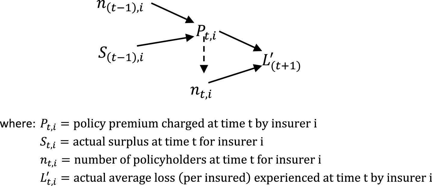
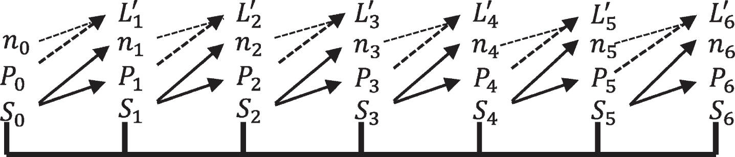
The property-liability insurance industry simulated here is comprised of C companies, who service an industry of N homogeneous customers. Insurance is mandatory and each company follows a simple pricing rule for determining the premium to charge all of its customers. The model operates in discreet time with insurers collecting premiums at time t while paying all losses at time (t + 1). Insurers charge a pure premium subject to a capacity consideration of a target capital structure. The insurers do not raise external capital. An insurer’s expected premium volume is based on the number of customers the insurer had the previous time period. The insurer’s actual premium volume is determined by a downward-sloping demand curve. A graphic of each year’s cash flows iteration is displayed in Fig. 1.2
Fig.1
A brief cash flow timeline.
2.1Target capital structure
It is assumed that each insurer desires to maintain a target capital structure, which may differ from insurer to insurer, and the only liabilities faced by each insurer are the total expected losses that are acquired when policies are sold. For example, if an insurer has a surplus of $2,000,000 and a target ratio of 40%,the insurer will desire to hold a total expected loss exposure of $3,000,000. The insurer will thereby collect a total (pure) premium of $3,000,000. Insurers do not engage in borrowing, or other forms of raising new capital.
When the simulation is initiated, each insurer starts in equilibrium with the same number of customers paying a premium equal to expected average loss. Each insurer is then given an initial surplus to match its desired capital structure. From this equilibrium starting point, the simulated insurers adjust their prices according to their respective surplus levels and most recent risk-pool size.
An insurer’s target capital structure, in this model, is representative of the insurer’s risk preference. Since the insureds are homogeneous, the target capital structure defines what level of loss exposure an insurer is willing to bear for a given amount of surplus. The beginning market equilibrium is an important ideal. Each experimental insurer has the exact total expected loss exposure it is willing to bear given its initial capital. Since the long-run equilibrium price gives an underwriting margin of zero, the long-run equilibrium objective of each insurer is to maintain its beginning surplus. An implication of this is when an insurer has excess capital, there is the incentive to set its price below the long-run equilibrium price, thus creating the possibility of a soft market. (See Harrington, Niehaus, and Yu (2013), page 659.) And when an insurer has a shortage of capital, it will set a price above the long-run equilibrium price. The premiums charged by each insurer, as well as the average price in the marketplace, will fluctuate around the long-run equilibriumprice.
As indicated in Fig. 1, and similar to Berger (1988), the capital structure numbers are subject to a one-year lag. Premiums at time t are, in part, a function of the surplus level at time (t - 1). The losses associated with these premiums are paid at time (t + 1).3 And keeping the cash flow lags in mind, and in accordance with the simplified capacity constraint model, each insurer’s desired level of loss exposure is a fixed ratio of the level of surplus.
2.2Downward sloping demand curve
In the simulated market insurance coverage is mandatory and modeled with a downward-sloping demand curve. These notions work together by assuming every insurer will maintain a minimal portion of the market and insureds, each year, are paying a range of prices for the same insurancecoverage.4
The number of insureds who buy a policy from the ith insurer is:
(1)
where:
This demand function is convex to the origin. The convexity increases with the range of prices. If prices are in a narrow range the demand curve appears quite linear. If an insurer charges an unusually large price, it will receive a very small proportion of customers. This style of demand curve is realistic. In practice, identical (or near identical) insurance policies are available at a range ofprices.
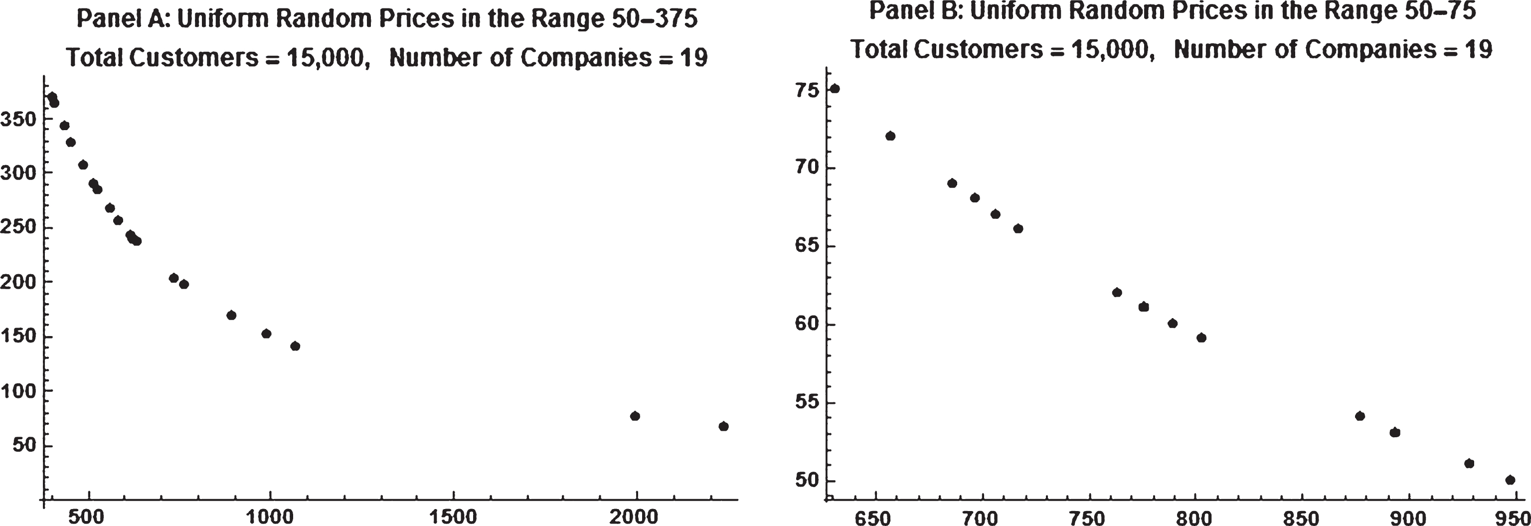
Figure 2 displays a generic example of the modeled demand curve. Each curve is based on a market of 15,000 customers and 19 companies. Panel A is computed from a wide range of prices ($50–$375), while Panel B is computed from a narrow price range ($50–$75). The convexity of the demand function is much more apparent in Panel A. The leftmost point in Panel A shows a price of $369, giving the company only 407 customers, the rightmost point in Panel A shows a price of $67 giving the company 2,240 customers. The leftmost point in Panel B has a price of $75 and 632 customers, while the rightmost point has the price of $50 giving 948customers.
Fig.2
Two examples of modeled demand curve.
2.3Expected losses
Each modeled insurance company’s losses are separately, and randomly, generated from an identical, stationary mixed loss distribution. Loss frequency is modeled as a Bernoulli variable with a 5% chance of loss. Loss severity is modeled (a little haphazardly) using the SkewNormalDistribution function in Mathematica with location parameter of 39,000, scale parameter of 30,000, and shape parameterof 55.
A series of losses is created for each company by multiplying, in pairwise fashion, each Bernoulli variable with a randomly generated severity number. This creates a list containing mostly zeros with a small proportion (expected to be 5%) of highly skewed losses.
2.4Simple pricing rule
The simple pricing rule constructed here is based on the idea of each insurer wanting to maintain a target capital structure,
For insurer i the target premiums-to-surplus ratio is7;
(2)
Rearranging Equation (2) gives;
(3)
Through time, each company’s actual average loss will deviate from expected. The number of actual policyholders will vary as well due to price competition and the downward-sloping demand curve. As these two deviations occur each insurer’s actual surplus will deviate from the target surplus. The pricing rule modeled here incorporates an adjustment term that attempts to account for the out-of-equilibrium surplus position. Each insurer will (likely) have a unique out-of-equilibrium position.
(4)
The first rhs term in Equation (4) is the target surplus for insurer i, at time t.
Given an insurer’s out-of-equilibrium position, as defined in Equation (4), and setting
(5)
Equation (5) is the model’s simple pricing rule. It is the expected average loss, L, plus the out-of-equilibrium position divided by n(t-1),i. The out-of-equilibrium position is divided by n(t-1),i to have the adjustment be on a per-policy basis.
2.4.1Considering
n t , i *
An insurer’s current surplus, St,i, is equal to the prior surplus, S(t-1),i, plus the profits (or losses) from the policies sold this year. This computation is;
(6)
The
3Simulation results
As with all simulations, specific results vary from run to run, yet some properties are identifiable across all runs. Of significance with this simple pricing-rule simulation is how skewness and kurtosis of the underwriting margin time series differ considerably across runs. That is, the shape of the apparent probability distribution of the simulated aggregate underwriting margin differs considerably from one experiment to the next. Using the fact that the real world underwriting margin data is a single realization, one can possibly conclude that certain continuous structural measures are not reliable broad-based pieces of analysis. The rule-based approach allows for different continuous probability structures to occur alongside other stable structural properties. The rule-based approach is looking for an algorithmic process.
The simulation results are presented by concentrating, primarily, on one specific representative outcome (referred to as Simulation X) that is interesting and typical. Other simulation runs, identified by number and reported in Appendix B, are referenced along the way.
3.1Simulation X
Simulation X created a property-liability insurance industry of 75 companies that operated for 200 years8. The target capital structures of these 75 companies are chosen randomly from a discrete uniform distribution containing the numbers {0.37, 0.38, 0.39, 0.40, 0.41, 0.42, 0.43, 0.44, 0.45, 0.46, 0.47, 0.48, 0.49, 0.50, 0.51, 0.52, 0.53, 0.54, 0.55}. The pricing rule, Equation (5), is subject to maximum increases and decreases. The maximum increase is 150%,while the maximum price decrease is 50%.These constraints are included to indicate (hypothetically) insurers are more hesitant to reduce prices drastically than increase them substantially. Figure 3, Panel A, shows the average underwriting margin for the simulated industry. The industry margin is a weighted average based on premiums.
It is clear in Fig. 3 that the cycle is drawn out. Casual counting from trough-to-trough gives a very typical length of 6 years – though it should be noted that the actual underwriting cycle is irregular. Figure 3, Panel B, displays the industry average loss, weighted by number of insureds. The losses are random with no cyclical-type behavior.
Fig.3
Underwriting margin and average loss, per insured, of simulated property-liability insurance industry (200 years).
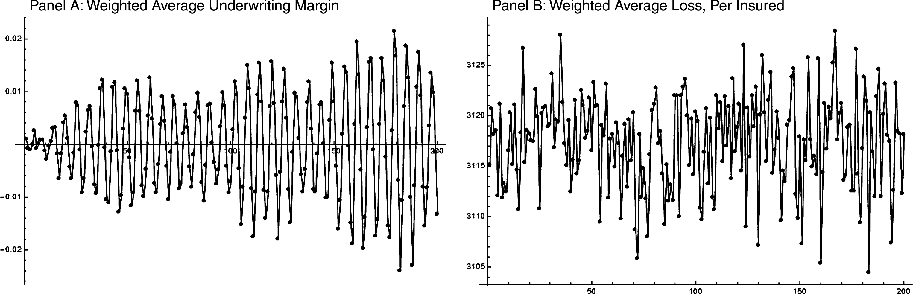
Table 1 presents summary data of the actual industry underwriting margin for 1930–2000. The aggregate data for the property-liability industry shows a negative average underwriting margin with greater volatility and skewness than the simulated data (Table 2). The negative aggregate margin can be an indication of expected losses being discounted to their present value (i.e. accounting for investment income). The greater volatility and skewness isn’t surprising considering the uncertainty of actual loss distributions.
Table 1
Summary statistics from U.S. stock property-liability insurers, 1930–2000
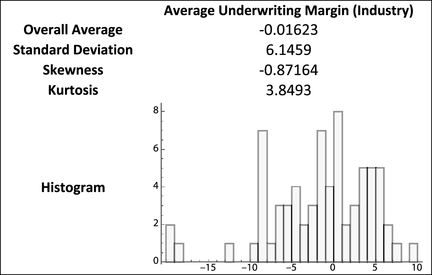 |
Table 2
Summary statistics from simulation X
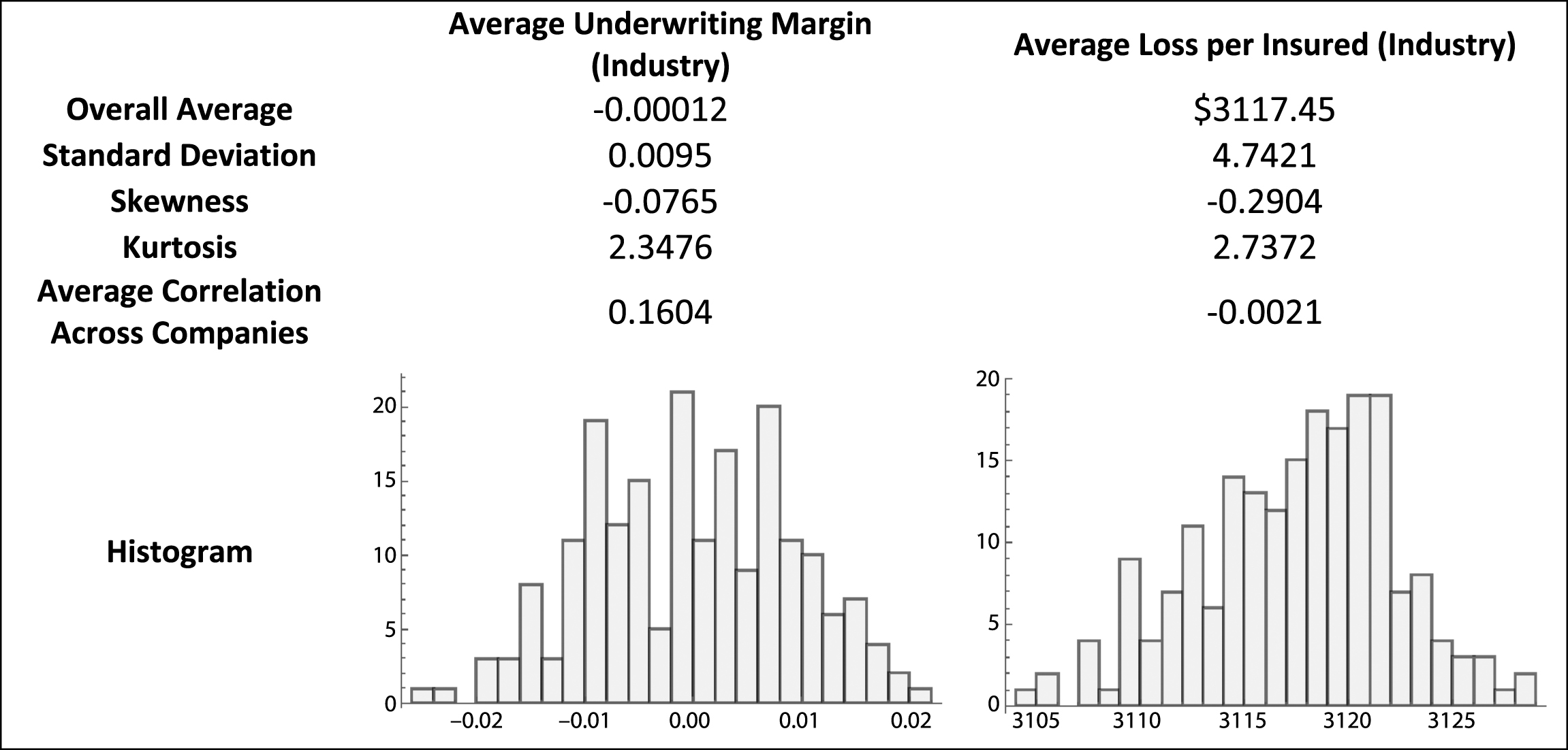 |
Table 2 contains summary statistics from Simulation X. The average underwriting margin of –0.00012 shows the simulated industry generally achieves equilibrium. The industry, on average, collects pure premium equal to losses paid. The distribution is quite narrow, nearly symmetrical, and a little platykurtic. The average correlation of underwriting margins across the 75 companies (2,775 terms) is slightly positive at 0.1604.
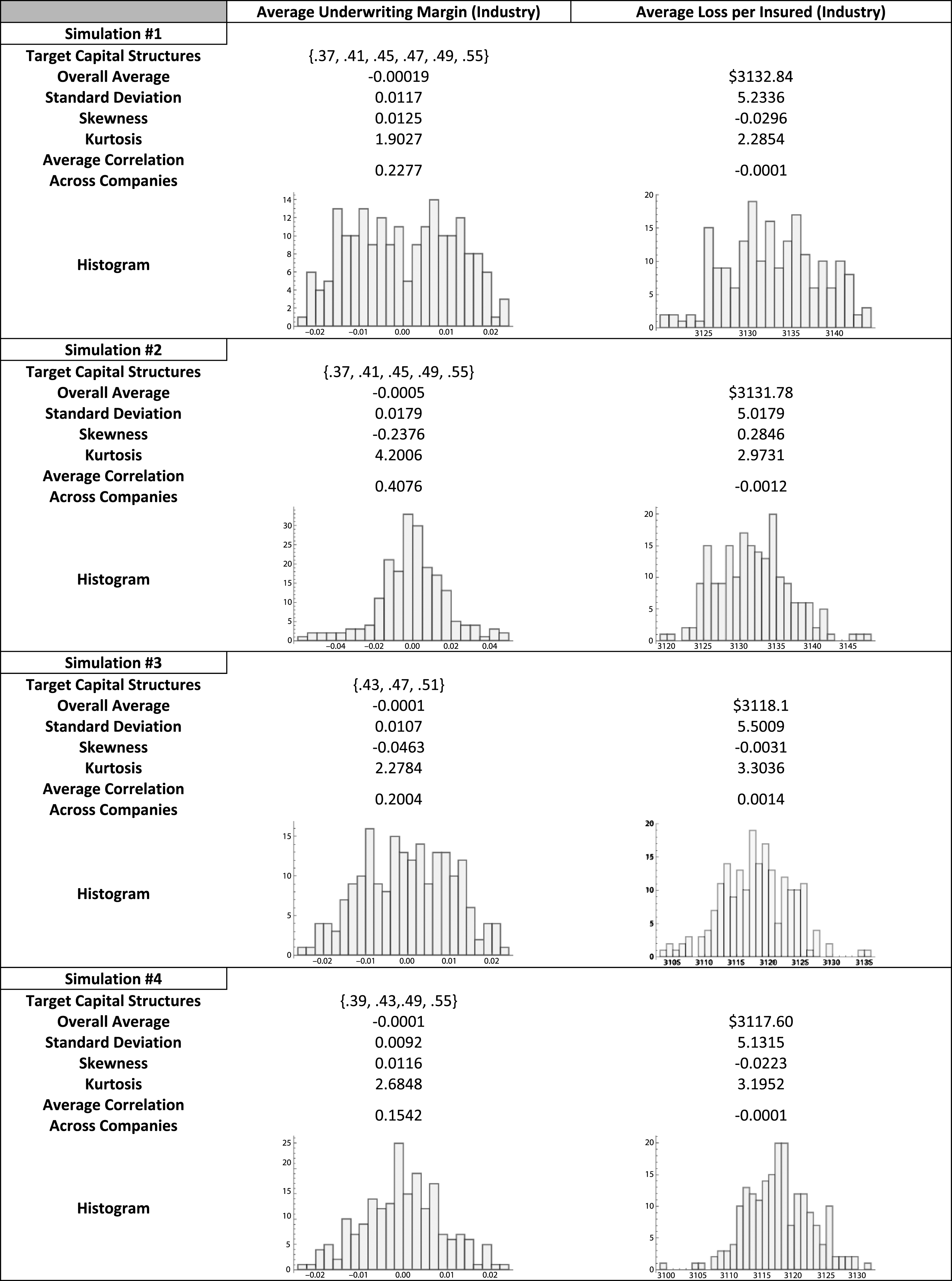
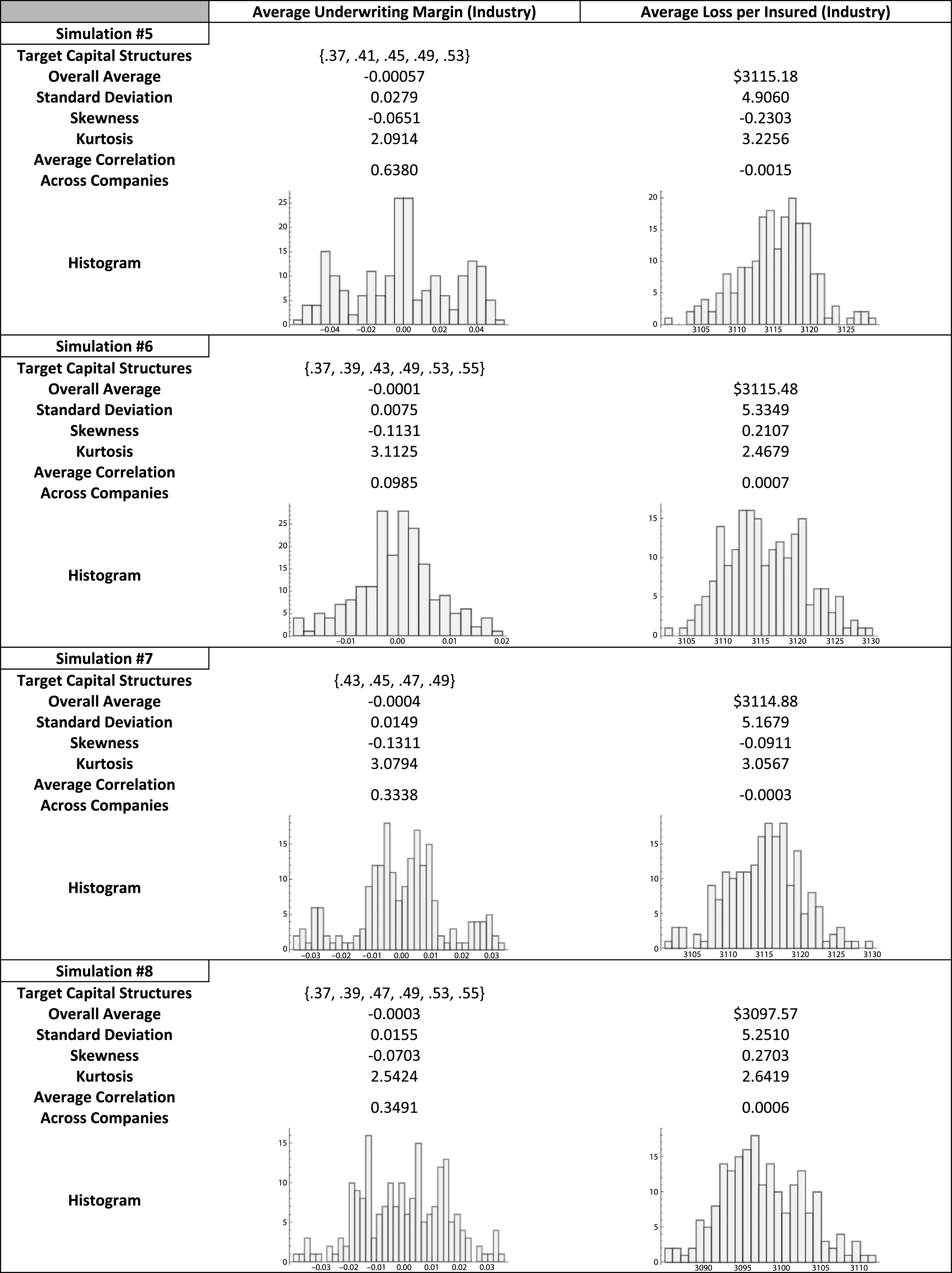
Eight additional runs of the simulation, displayed in Table 1B of Appendix B, show a variety of distributional outcomes for the aggregate underwriting margin. All of the histograms are centered (essentially) on zero, indicating the simulated market’s effort to achieve equilibrium, while the shape of the histograms differ significantly. When one considers the fact that only one outcome is actually realized through time, e.g., Table 1, it can be concluded that analyzing the distributional shape of the realized outcome may be misleading.
3.2Directional bit sequences
Zenil and Delahaye (2011) show that directional bit sequences are another way to look for a consistent structure across all possible realizations. Directional bit sequences are constructed by looking at the directional changes from observation to observation. Using the notation, 0 = down and 1 = up, any time series can be converted into a directional bit sequence. For example, in Simulation X, the first seven aggregate average underwriting margin outcomes are {0.091%,–0.084%,–0.105%,–0.002%,0.264%,–0.075%,–0.002% }.9 This sequence generates three 4-tuple directional bit sequences {0,0,1,1}, {0,1,1,0}, {1,1,0,1}. The first directional bit sequence represents changes from t = 1 through t = 5. These changes are {down, down, up, up}. Each successive bit sequence is created by shifting the starting point one time period.
A 4-tuple bit sequence has 24 = 16 possible outcomes. Any time series, real or simulated, can be converted to directional bit sequences from which a set of probabilities can be determined indicating the frequency with which each possible sequence occurs. These probabilities present a different way of analyzing the structure of a time series.
3.3Comparing simulation X to ‘real world’ data using directional bit sequences
4-tuple directional bit sequences were compiled from the actual underwriting margin data and Simulation X results. The actual data has 71 observations and therefore generated 67 four-tuple bit sequences, while Simulation X has 200 observations and 196 four-tuple sequences. Table 3 presents the probabilities of each possible sequence for the two data series. The probabilities are graphed in Fig. 4.
Table 3
Directional bit sequence probabilities for the actual and simulated underwriting margin
| Point on | Bit | Actual | Simulated |
| Figure 6 | Sequence | Underwriting | Underwriting |
| Margin | Margin | ||
| Probability | Probability | ||
| (n = 67) | (n = 196) | ||
| 1 | {1,1,1,1} | 0.0000 | 0.0153 |
| 2 | {1,1,1,0} | 0.1045 | 0.1429 |
| 3 | {1,1,0,1} | 0.0299 | 0.0051 |
| 4 | {1,1,0,0} | 0.1343 | 0.1684 |
| 5 | {1,0,1,1} | 0.0299 | 0.0051 |
| 6 | {1,0,1,0} | 0.0299 | 0.0000 |
| 7 | {1,0,0,1} | 0.0299 | 0.0255 |
| 8 | {1,0,0,0} | 0.1194 | 0.1429 |
| 9 | {0,1,1,1} | 0.0896 | 0.1429 |
| 10 | {0,1,1,0} | 0.0597 | 0.0306 |
| 11 | {0,1,0,1} | 0.0299 | 0.0000 |
| 12 | {0,1,0,0} | 0.0149 | 0.0000 |
| 13 | {0,0,1,1} | 0.1194 | 0.1684 |
| 14 | {0,0,1,0} | 0.0149 | 0.0000 |
| 15 | {0,0,0,1} | 0.1045 | 0.1378 |
| 16 | {0,0,0,0} | 0.0896 | 0.0153 |
Fig.4
Probabilities of All Possible 4-tuple directional bit sequences.
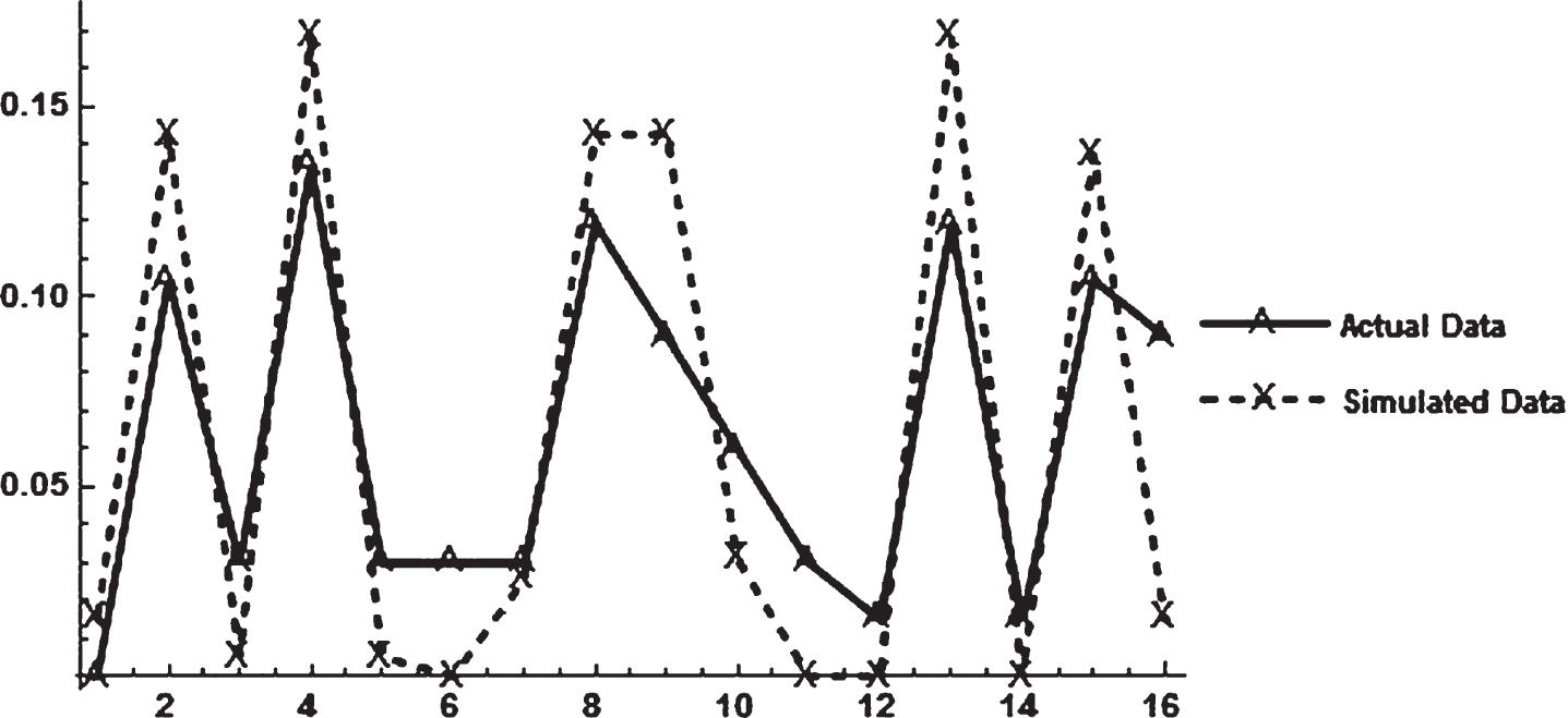
The plotted points in Fig. 4 clearly form similar shapes10. The correlation between the probability sets is 0.9053. It appears the structure of the simulated data is quite similar to the structure of the actual data.
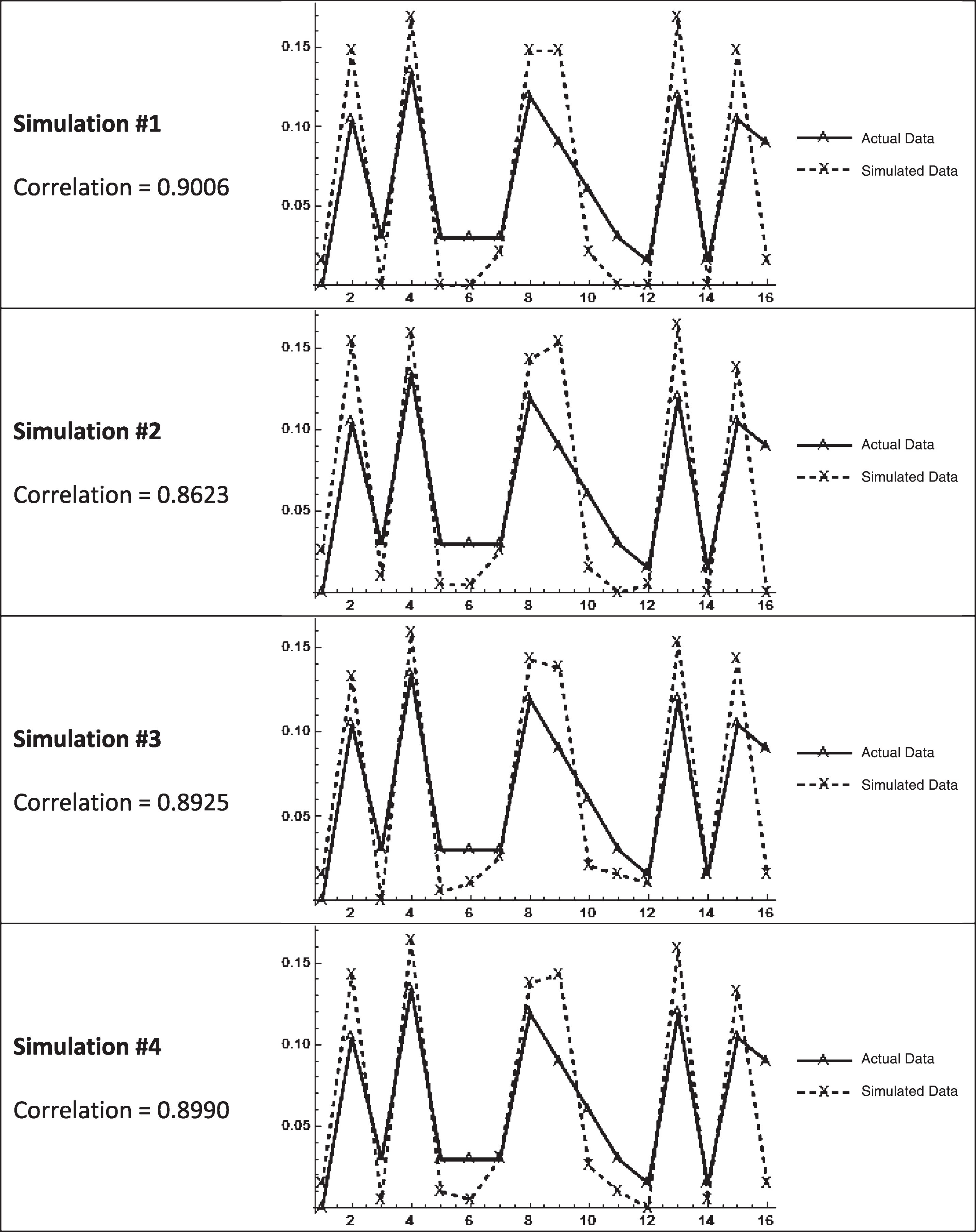
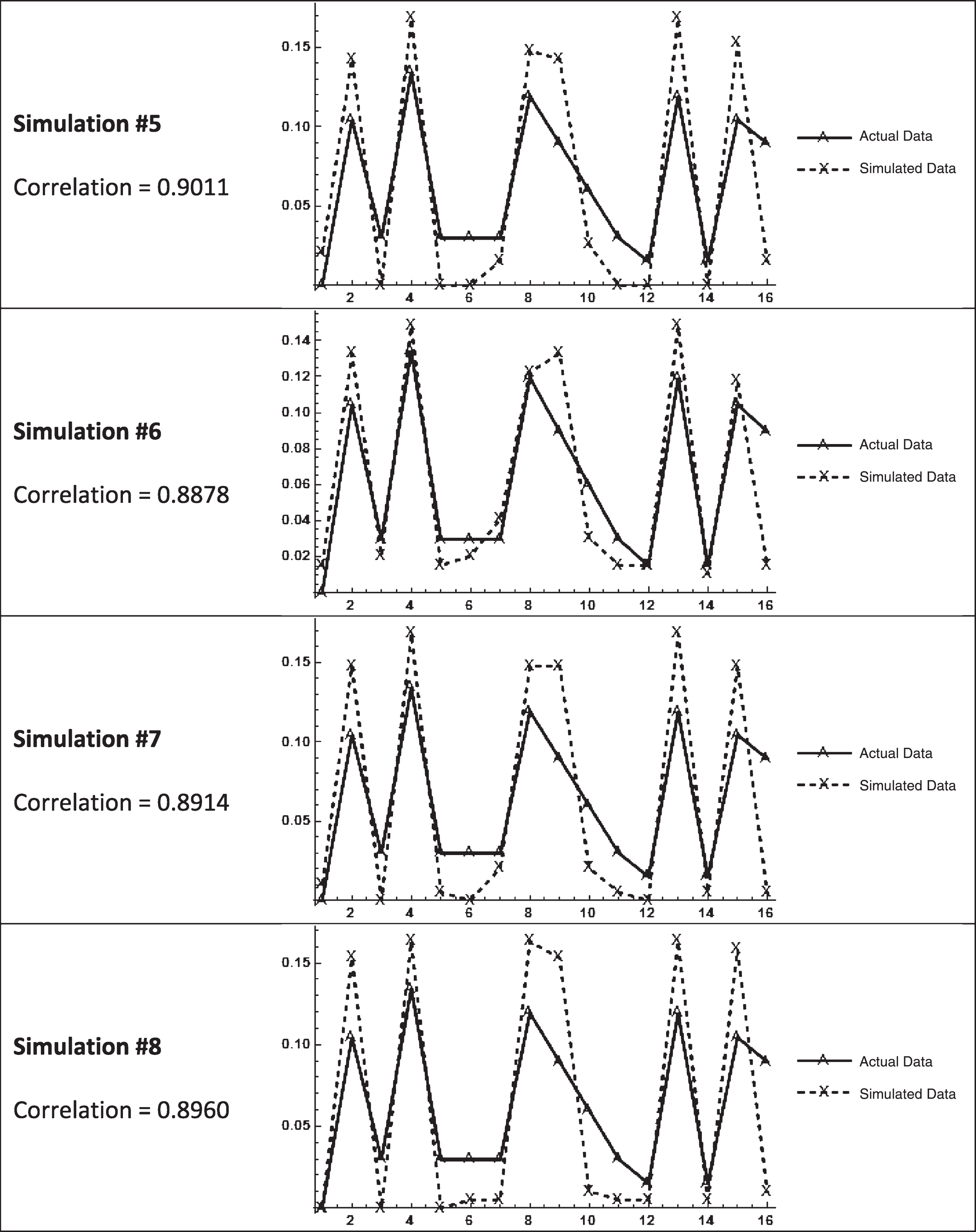
Table 2B in Appendix B contains the directional bit sequence probability plots of the average underwriting margin for the eight additional simulations. All of these simulations reveal probabilities with high correlation to those of the actual underwriting margin directional bit sequences.
The matching structure of directional bit sequences between multiple runs of simulated data and the actual underwriting margin lends strong support to the property-liability insurance industry following an algorithmic process. The simulation shows the simple discrete-time pricing rule moving the industry towards equilibrium while generating a simulated aggregate underwriting cycle possessing much of the same structure as the actual underwriting cycle. The rule is a simple-as-can-be algorithm that has each company determine Pt from S(t-1) and n(t-1).
3.3.1Behavior of individual companies’ directional bit sequences
With each individual insurer following the simple pricing rule and the simulated aggregate underwriting margin possessing a directional bit sequence structure very similar to the actual industry underwriting margin, an obvious question to ask is ‘what is the structure of the directional bit sequences of the underwriting margins of the individual companies?’
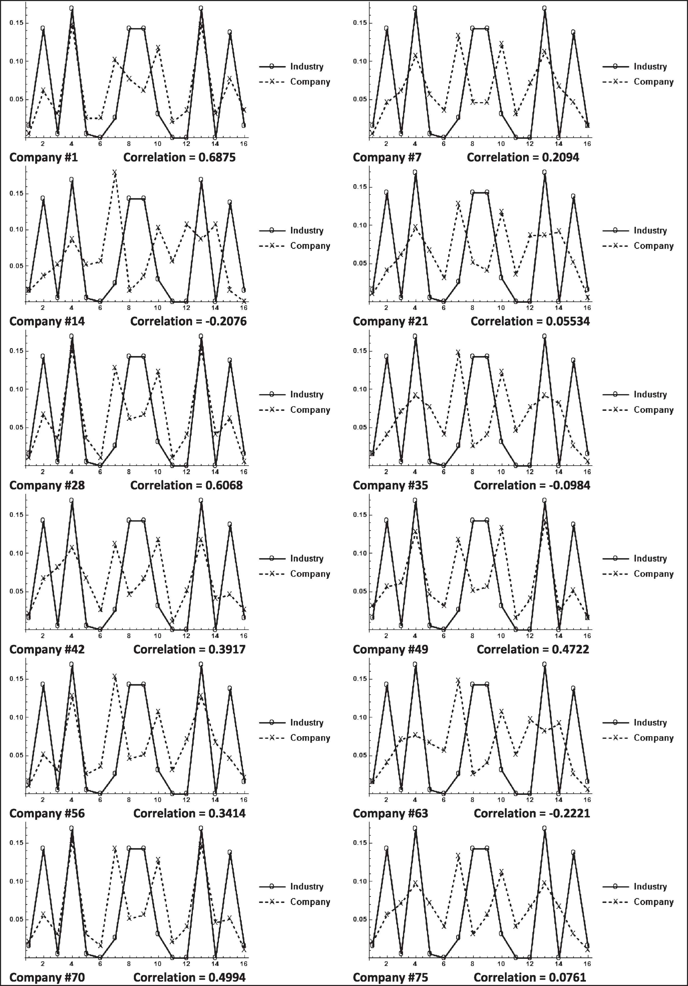
Table 4 contains the directional bit sequence probability plots of companies {1, 7, 14, 21, 28, 35, 42, 49, 56, 63, 70, and 75}.11. The individual company plots show a wide range of outcomes when compared to the simulated industry underwriting margin. The correlations range from –0.2076 to 0.6875. The directional bit sequences of individual company underwriting margins do not, in general, have the same structure as the sequences of the simulated industry margin.
Table 4
Directional bit sequence probability plots for 12 companies in simulation X
 |
3.4Emergent behavior
Can the behavior of the directional bit sequences of the aggregate underwriting margin be considered emergent behavior? Maybe, maybe not. While acknowledging that “emergence is a property without a sharp demarcation” Holland (2013, page 4) prefers to concentrate “on interactions where the aggregate exhibits properties not attained by summation”12. The aggregate underwriting margin is a weighted average, based on premium volume, of the individual company underwriting margins. However, the aggregate directional bit sequence probabilities are not an average of the individual bit sequence probabilities.
Page (2012) discusses emergent behavior as an aggregate property not exhibited by individual agents. This appears to mostly be the case in Simulation X. Of the 12 companies listed in Table 4, only two of them have directional bit string correlations greater than 0.5.
3.5Randomness
It is important to distinguish randomness from the matching structure discovered between the algorithmic simulated data and the actual data. This is done by converting randomly generated time series to directional bit sequences. Table 5 contains correlation coefficients for the directional bit sequences of randomly generated time series from four continuous probability distributions –the normal distribution, beta distribution, uniform distribution, and Cauchy distribution. It is clear that all distributions generated nearly identical discrete 4-tuple bit sequence probabilities.
Table 5
Correlations of directional bit sequence probabilities from random times series (n = 100,000)
| Normal | Beta | Uniform | Cauchy | |
| distribution | distribution | distribution | distribution | |
| Normal | ||||
| Distribution | 1 | 0.9997 | 0.9999 | 0.9996 |
| Beta | ||||
| Distribution | 1 | 0.9996 | 0.9999 | |
| Uniform | ||||
| Distribution | 1 | 0.9995 | ||
| Cauchy | ||||
| Distribution | 1 |
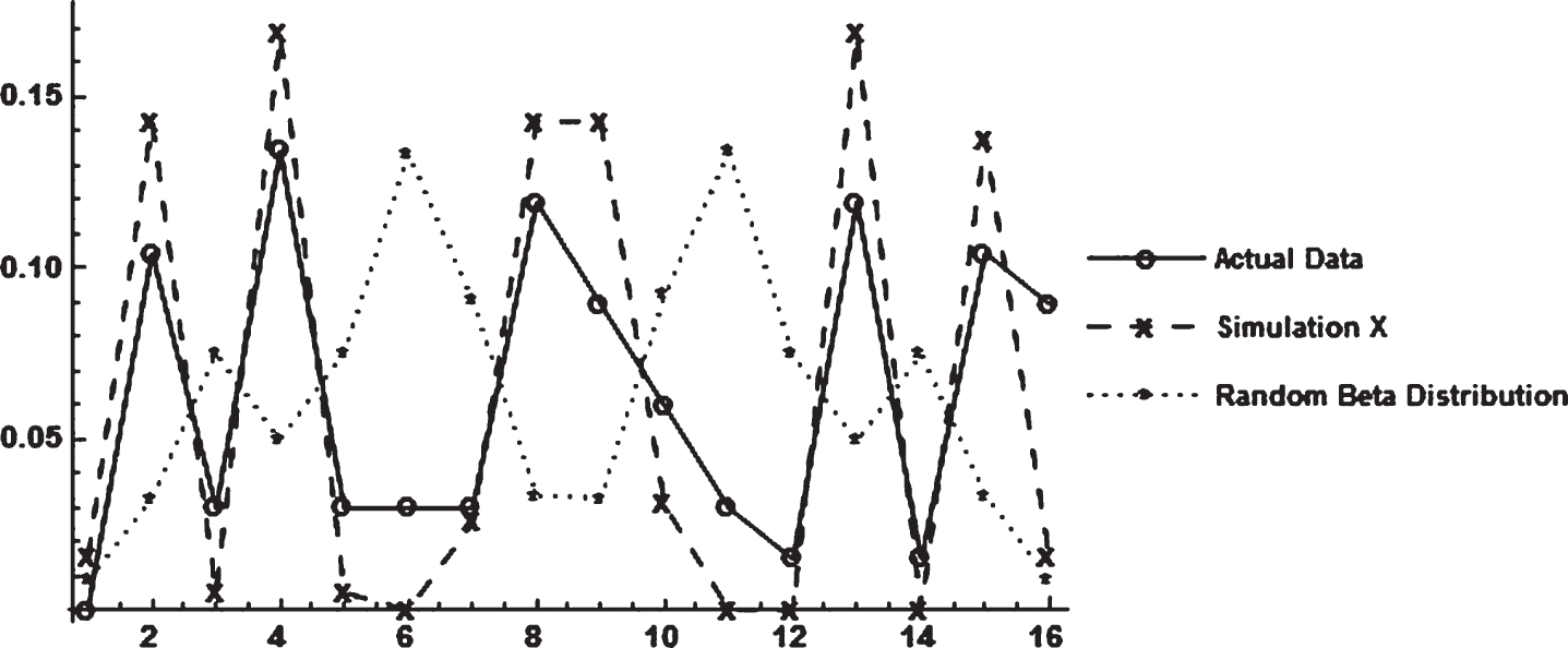
Figure 5 overlays the directional bit sequences of the random beta distribution with the directional bit sequences from the actual aggregate underwriting margin and the simulated industry margin. The bit sequences from the random series is clearly distinct from the other two series.
Fig.5
Directional bit sequence probabilities from several time series.
3.6Observations on correlated behavior amongst the simulated insurers
The results of Simulation X and the other eight simulations show higher standard deviations of the aggregate underwriting margin associated with higher average underwriting margin correlations across all 75 companies (Tables 2 and 1B). To further investigate this another 27 simulations were run. Nine simulations each for pretend insurance industries of sizes 55 companies, 35 companies, and 15 companies. The results are displayed in Fig. 6.
Fig.6
The Relationship between the Standard Deviation of Simulated Underwriting Margins and the Average Correlation of Simulated Underwriting Margins across Multiple Companies.
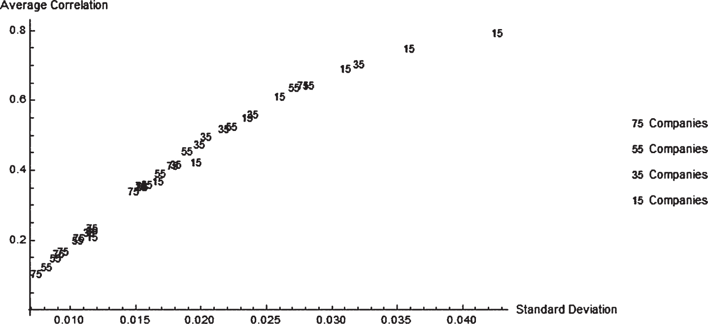
Figure 6 shows that higher standard deviations of company underwriting margins are associated with higher average correlation across companies. Figure 6 also shows that industries with fewer companies tend to be associated with both higher volatility and correlations.
Simulation #7, in which the aggregate underwriting margin becomes more volatile around t = 125, provides another perspective on the relationship of increased correlation across companies during periods of higher volatility. The average correlation across companies for the entire Simulation #7 is 0.3338. Table 6 displays the results of splitting the 200 time periods into two subsections, t = 1–125 and t = 126–200. The sub-period with greater volatility, t = 126–200, also has a greater correlation amongst the simulated companies’ underwriting margins.
Table 6
Aggregate underwriting margin statistics after splitting simulation #7 into two sub-periods
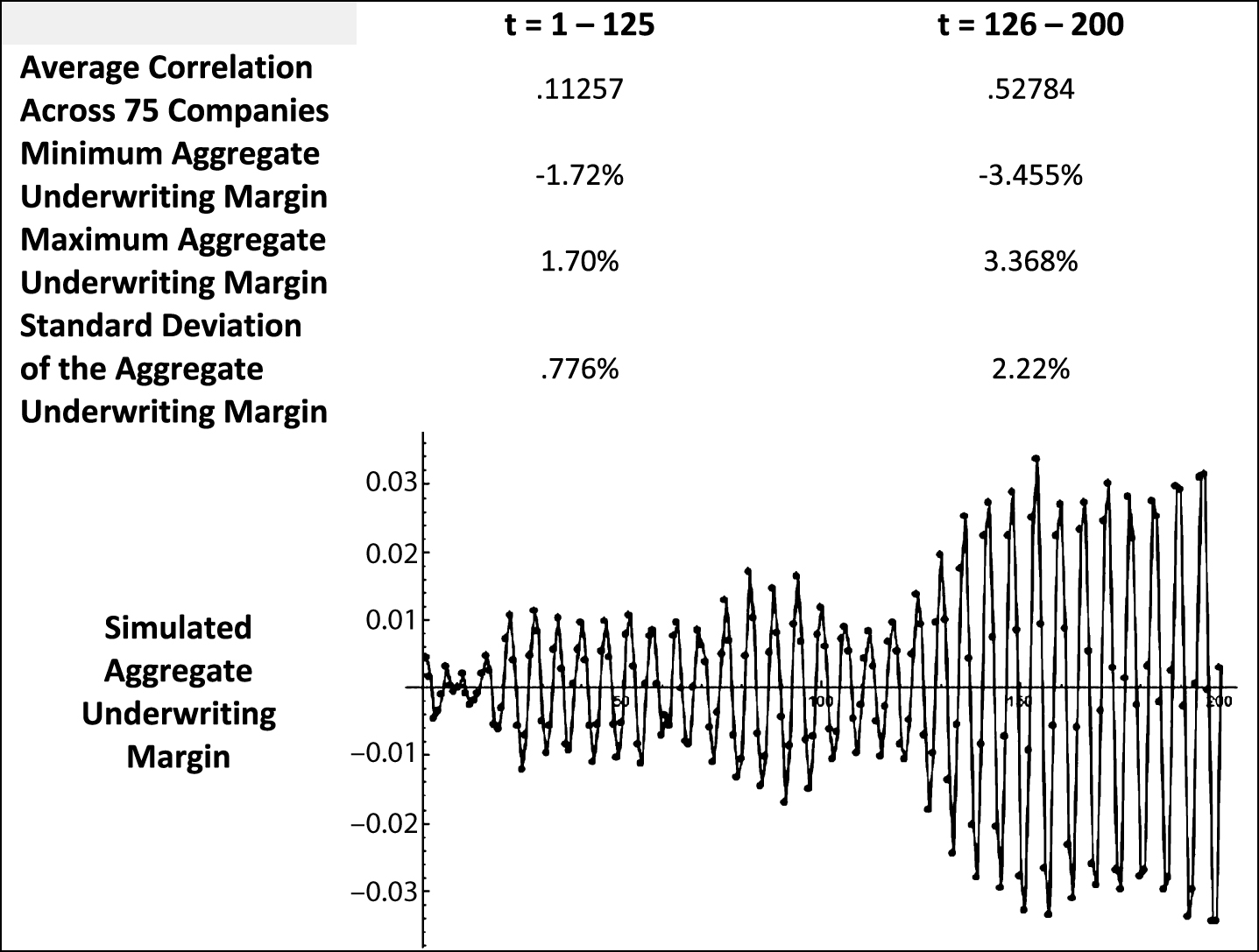 |
Observing periods of higher correlation across companies being associated with greater volatility makes economic sense. Although a company’s underwriting margin is subject to the randomness of insured losses, it can still be considered a proxy for price. During periods of higher price volatility companies will tend to behave in what appears to be a more coordinated manner. If price-cutting during a drawn out soft market becomes severe enough almost all companies have to participate to avoid having their risk-pools shrink significantly. (The so-called ‘race to the bottom’.) After a period of strong price-cutting, all companies eventually need to recover surplus by raising prices.
The graph in Table 6 shows relatively mild underwriting cycles for 125 time periods. Insurer’s underwriting margins (prices) during these 125 periods have low correlation indicating the companies are competing yet behaving independently. The last 75 time periods are different however. The margin fluctuations are larger and the companies’ behavior is more correlated.
The additional outcome of a market with fewer companies having greater correlated activity (Fig. 6) also makes economic sense. Competition, generally, is greater with more companies in an industry and the greater the competitive behavior the lower the correlated activity.
4Concluding comments
This paper presents a computational economics model, and experiment, showing the property-liability insurance industry following a simple algorithmic process. The simple algorithmic process has individual insurers base their premium on expected average loss and, with a one-year lag, the size of their risk-pool and level of policyholders’ surplus. There is also a one-year lag between premiums collected and payment of actual losses. This simple algorithm does not have an adaptive, or learning, feature. The insurers repetitively apply the same pricing rule year after year.
The model is an agent-based explanation of market behavior that reveals a common structure between the simulated and observed data with the use of directional bit sequences. The directional bit sequence probabilities of Simulation X, as well as the eight other simulations reported in Appendix B, are all highly correlated with the actual property-liability aggregate underwriting margin, 1930–2000.
Finding this discrete common structure and asserting a simple algorithmic process at least partially removes the value of determining what sort of continuous probability distribution governs the DGP of the aggregate underwriting margin. The histograms presented in Tables 2 and 1B show a wide variety of shapes on the probability distributions of the simulated underwriting margins. Relaxing the constraint of a continuous DGP on the time series opens the analysis by separating the pursuit of equilibrium from the movement around equilibrium.
4.1Pursuit of equilibrium
Haley (1993, 2007) uses cointegration methodology to conclude the property-liability insurance industry consistently pursues equilibrium. The studies show there is a linear equilibrium attractor between the aggregate underwriting margin and the 90-day T-bill rate.13 These studies, however, do not offer any description of behavior around the equilibrium attractor other than mean stationarity of (error term) deviations from equilibrium, i.e. the underwriting margin has the tendency to move towards equilibrium.
The algorithmic pricing process demonstrated here shows that it is unnecessary to determine a definite continuous DGP for a time series when evaluating equilibrium behavior. Any continuous DGP that appears will be temporary. Economic circumstances will eventually lead to a structural change. Studying structural DGP changes are of significance in a historical context, but are not needed when determining the existence of equilibrium behavior.
One key mechanical component of the modeled market’s pursuit of equilibrium is its agent-based construct. This construct of individual actions leading to the aggregate pursuit of equilibrium, according to Farmer and Geanakoplos (2008), is an important feature of equilibrium theory. A second key mechanical component of the modeled market is the downward-sloping demand curve. After each insurer sets its price, the demand curve allocates the population of insureds across companies. In each time period, insurance coverage is sold along the demand curve at a range of prices. Virtually all of these transactions occur out-of-equilibrium in the sense that the transacted prices deviate from the intersection point of aggregate supply and aggregate demand. The simulated market perpetually pursues equilibrium, yet never settles on it.
Equilibrium, whether evaluated as a point or some higher-dimensional attractor space, has a gravity-like pull on economic activity. However, due to the myriad exogenous factors typical of even narrow economic settings, the gravity-like pull of equilibrium is not uniform (or symmetrical) across time. In one circumstance, a deviation from equilibrium may be adjusted to rapidly, whereas another circumstance may result in slow adjustment. The directional bit sequences presented here provide an analysis tool whereby the probabilities of specific directional change patterns, not the momentum of changes, can be compared between times series.
Analyzing direction of change separately from magnitude of changes is a stronger statement than simply acknowledging heteroscedasticity, e.g. ARCH-type models. In a rule-based system with time series not governed by a continuous DGP, separating the analysis of direction and momentum explicitly acknowledges that the two phenomena are independent of one another.
4.2Volatility and competition
The individual companies of this experimental insurance industry, who are repetitively applying the simple pricing rule described by Equation (5), possess some intuitively appealing outcomes. First, the behavior of the companies, when evaluated as directional bit sequences, tend to be uncorrelated with the behavior of the industry. This can be compared to the classic bird flocking example of emergent behavior. Individual companies are following the simple pricing rule, are connected via the downward-sloping demand curve, and exhibit an aggregate behavior apart from that of the individuals.
A second economic outcome is that company behavior is more correlated during periods of volatility. Volatility changes in the simulation are endogenous with no obvious cause. The higher correlation amongst companies during periods of higher volatility, however, is clear. The economic interpretation of this increased correlation holds that companies eventually have to participate in large price reductions or risk losing customers.
A final note on company behavior in this simulated insurance industry –industries with fewer companies tend to display more correlated behavior and more volatility. Fewer companies in an industry is indicative of a less competitive market.
4.3Future research
One direction for future research is to build on the computational model presented here and provide further explanation of the movement of the aggregate underwriting margin around the equilibrium attractor. A second, more general, direction for future research is to determine if the computational thinking of rule-based decisions and directional bit sequences applies to other markets/industries. And finally, a third avenue for future research is to use the directional bit sequence probabilities to develop a predictive model.
Appendices
Appendix A
Modeled Cash Flows for t = 0 through t = 5. (Company #1 from Simulation X)
Appendix C describes the loss generating function and the parameters used. The theoretical expected annual loss, per insured, is $3,123.59. All simulation runs are initialized by giving each insurer a risk pool of size, n0 = 100, 000, and an identical initial premium. The initial premium is equal to the average of 2,000,000 simulated loss observations.
| t = 0 | Three values initialize the simulation |
| P0 = $3, 118 | P0 = L = $3, 118 ≈ $3, 123.59 |
| n0 = 100, 000 | n0= starting value of 100,000 insureds |
| S0 = $235, 217, 544 |
|
| the insurer’s desired
| |
| t = 1 | |
| P1 = $3, 118 |
|
| n1 = 100, 000 | n1 is determined using Equation (1) with P1 = $3, 118. |
| = the average of n1 randomly generated losses. | |
| S1 = $232, 117, 544 | |
| t = 2 | |
| P2 = $3, 149 |
|
| n2 = 98, 902 | n2 is determined using Equation (1) with P2 = $3, 149. |
| = the average of n1 randomly generated losses. | |
| S2 = $227, 917, 544 | |
| t = 3 | |
| P3 = $3, 165.70 |
|
| n3 = 98, 520 | n3 is determined using Equation (1) with P3 = $3, 165.70. |
| = the average of n2 randomly generated losses. | |
| S3 = $230, 785, 702 | |
| t = 4 | |
| P4 = $3, 127.65 |
|
| n4 = 99, 763 | n4 is determined using Equation (1) with P4 = $3, 127.65. |
| = the average of n3 randomly generated losses. | |
| S4 = $241, 888, 593 |
Appendix B Table 1B:
Summary Statistics from Simulations #1 through #8
 |
 |
Appendix B Table 2B:
Directional Bit Sequence Probabilities for Aggregate Underwriting Margin from Simulations #1 through #8
 |
 |
Appendix C –Losses generated
Losses are generated for each company using a mixed distribution of frequency and severity. Frequency is modeled by a Bernoulli distribution with 5% probability of ‘success’. Severity is modeled using the SkewNormalDistribution [39,000, 30,000, 5] function in Mathematica.
Each component distribution generates a list of 2,000,000 random numbers. These lists are multiplied, in pairwise fashion, to generate a list of possible losses. A 15 element sample list of losses is presented in Figure 1C.
Figure 1C: A 15 Element Sample of the Mixing Distribution for Random Loss Generation
For each simulated company, each year, ni random losses are chosen from the list of 2,000,000 potential losses. Most of the list is, of course, zeros. These individual losses, however, are not recorded as part of the simulation, only the average loss, per insured, for each company is recorded.
C.1Theoretical parameters
The mean, variance, and standard deviation of the 5% Bernoulli distribution are;
(1A)
(2A)
(3A)
The mean, variance, and standard deviation of the SkewNormalDistribution function are;
(4A)
(5A)
(6A)
The mean, variance, and standard deviation of the mixed distribution of losses are;
(7A)
(8A)
(9A)
The simulated industry average loss numbers reported in Tables 2 and 1B are from a sampling distribution of sample size 7,500,000. (That is 75 companies, and a starting value of 100,000 insureds per company.) The mean, variance, and standard deviation of this sampling distribution are;
(10A)
(11A)
(12A)
These theoretical numbers correspond reasonably well to the numbers reported in Tables 2 and 1B.
Each company’s losses are a sampling distribution of approximate sample size 100,000. The actual sample size varies from year to year. Fixing the sample size at 100,000, the mean, variance, and standard deviation of each company’s sampling distribution are;
(13A)
(14A)
(15A)
As mentioned earlier, the individual losses for individual companies are not tracked in the simulation. Only the average loss per insured, per company is recorded.
Notes
1 The ability to supply insurance is, of course, also based the insurer’s ability to predict losses. It is assumed here that an insurer is able to predict losses with reasonable accuracy.
2 It needs to be noted that, at any point in time, the determination of Pt is done prior to
3 A detailed timeline of modeled cash flows for t = 0 through t = 5 is provided in Appendix A.
4 The dashed arrow in Fig. 1 is an effort to indicate the workings of the demand function shown in Equation (1).
5 The goal of modeling loss severity was to create a highly and positively skewed set of possible losses. I arbitrarily selected the parameters for the SkewNormalDistribution. More details are provided in Appendix C. More information about SkewNormalDistribution can be found at reference.wolfram.com.
6 Since each insurer faces identical, stationery loss distributions, incorporating a risk (profit) load factor based on the variance of expected losses would only result in a scalar adjustment to the simulation’s results.
7 Given the assumption of all losses being paid at the end of each year, the premiums-to-surplus ratio is also the debt-equity ratio.
8 As noted earlier and in Appendix A, the simulations are initiated by assigning arbitrary values to S0, P0, and n0 that have each insurer start in equilibrium. The description and analysis of results does not include the t = 0 values.
9 The t = 0 time period is dropped from the simulated insurance market series.
10 The points plotted are discreet. The connecting lines are drawn to aid interpretation. Directional bit sequence probabilities were computed and plotted to sequences of length 2, 3, 5, and 6. The results were qualitatively similar to the 4-tuple bit sequences.
11 I arbitrarily chose the first company, the last company, and those that are multiples of seven. The companies are not ‘cherry-picked’
12 See also, Holland (1995) pages 10-12, and page 125.
13 Haley (1995) demonstrates the cointegration between underwriting margin and 90-day T-bill rate exists for only a subset of individual insurance lines.
Acknowledgments
The author would like to acknowledge the help and encouragement of Stephen Wolfram, Matthew Szudzik, Hector Zenil, and all the participants of the 2013 Wolfram Science Summer School. I would also like to thank the editor, Philip Maymin, and an anonymous reviewer for very helpful comments.
References
1 | Berger L. , (1988) . A model of the underwriting cycle in the property/liability insurance industry, The Journal of Risk and Insurance 55: (2), 298–306. |
2 | Farmer J.D. , Geanakoplos J. , (2008) . The virtues and vices of equilibrium and the future of financial economics, Complexity 14: (3), 11–38. |
3 | Gron A. , (1994) . Capacity constraints and cycles in property-casualty insurance markets, RAND Journal of Economics 25: (1), 110–127. |
4 | Haley J.D. , (1993) . A Cointegration analysis of the relationship between underwriting margins and interest rates: 1930-1989, The Journal of Risk and Insurance 60: (3), 480–493. |
5 | Haley J.D. , (1995) . A by-line cointegration analysis of underwriting margins and interest rates in the property-liability insurance industrye, The Journal of Risk and Insuranc 62: (4), 755–763. |
6 | Haley J.D. , (2007) . Further considerations of underwriting margins, interest rates, stability, stationarity, cointegration, and time trends, Journal of Insurance Issues 30: (1), 62–75. |
7 | Harrington S. , Niehaus G. , Yu T. , (2013) . Insurance PriceVolatility and Underwriting Cycles, in Handbook of Insurance, 2nd edition, Dionne G. , editor, (Springer). |
8 | Holland J. , (1995) . Hidden Order, (Addison-Wesley). |
9 | Holland J. , (2013) . Complexity: A Very Short Introduction, (Oxford). |
10 | Page S.E. , (2012) . Aggregation in agent-based models of economies, The Knowledge Engineering Review 27: , 151–162. |
11 | Winter R.A. , (1994) . The dynamics of competitive insurance markets, Journal of Financial Intermediation 3: (4), 379–415. |
12 | Zenil H. , Delahaye J.-P. , (2011) . An algorithmicinformation-theoretic approach to the behavior of financialmarkets, Journal of Economic Surveys 25: (3), 431–463. |


