
The comparison of significance of fuzzy community partition across optimization methods
Abstract
The analysis of fuzzy(overlapping) community structure in complex networks is an important problem in data mining of network data sets. However, due to the exist of random factors and error edges in real networks, how to measure the significance of community structure efficiently is a crucial question. In this paper, we present a novel statistical framework comparing the significance of fuzzy community structure across various optimization models. Different from the universal approaches, we calculate the similarity between a given node and its leader and employ the distribution of link tightness to derive the significance score, instead of a direct comparison to a randomized model. Based on the distribution of community tightness, a new “p-value” form significance measure is proposed for community structure analysis. Specially, the well-known approaches and their corresponding quality functions are unified to a novel general formulation, which facilitate providing a detail comparison across them. To determine the position of leaders and their corresponding followers, an efficient algorithm is proposed based on the spectral theory. Finally, we apply the significance analysis to some famous benchmark networks and the good performance verified the effectiveness and efficiency of our framework.
1Introduction
A common feature observed in real networks is the presence of community structures [1–5, 18], i.e. subgraphs which are densely connected to each other while less connected to the subgraphs outside. In many scenarios, nodes in a network can belong to more than one community, called fuzzy(overlapping) communities [2–9]. In order to estimate how much a decomposition of a network which is found by a community detection algorithm is meaningful, we need a quality measure. Consequently, for a particular measure, the community detection algorithms can be ranked. To this end, various measures have been proposed in the literature, so far. The most prevalent measure which has been used extensively in the literature is due to Newman and Girvan [18]. This measure, called modularity, quantifies how much the density of the edges inside identified communities differs from the expected edge density in an equivalent network with similar number of vertices and edges but randomized edge placement, which is taken as the null model for statistical tests. Considering the modularity measure, the community detection problem is transformed to the modularity maximization problem. Modularity function can naturally extended to fuzzy form, which used to detect overlapping communities.
Recently, some optimization algorithms based on Potts models which used to detect community structure have attracted attention. Communities correspond to Potts model spin states, and the associated system energy indicates the quality of a candidate partition. It models an inhomogeneous ferromagnetic system where each node is viewed as a labeled spin in the network. Let A be the adjacency matrix of graph G and let σ i denote the label of the community that node i belongs to. Furthermore, the Kronecker Delta function is defined by δ (σ i , σ j ) =1 if σ i = σ j and δ (σ i , σ j ) =0, otherwise. Having the community membership labels σ, Reichardt and Bornholdt (RB) [16] proposed a generalized Hamiltonian as the core energy function,
(1)
Label propagation is another famous algorithm for community detection [27]. Briefly, the algorithm starts with randomly assigning a community label to each node. Then, each node updates its label by replacing it by the label most used by its neighbors. The other well-known optimization approaches used in community detection problem are Simulated Annealing (SA) [25], extermal optimization (DA) [13], expectation maximization [20], Bayesian inference [17], and variational Bayes [15]. For a comprehensive and comparative review on this topic we refer the reader to [4].
Although a lot of optimization method and their functions are proposed, How to determine the hidden properties of a given community [9] effectively remain unclearly answered. To answers these crucial questions, in this paper, we present a novel statistical framework comparing the significance of soft community structure across various optimization methods. Different from the universal approaches, we calculate the similarity of a given node to its leader and employ the distribution of link tightness to derive the significance score, instead of a direct comparison to a randomized model. A small example is shown in Fig. 1a, which illustrates that tighter the following nodes link to its leader, more significant the community is. Based on the distribution of community tightness, a new “p-value” form significance measure is proposed for community structure analysis. Specially, the well-known approaches and their corresponding quality functions are unified to a novel general fuzzy formulation, to provide a detail comparison across them. Then, we can choose the most suitable form of the function by set the parameters properly. To determine the position of leaders and their corresponding followers, an efficient fuzzy detection algorithm is proposed based on the spectral theory. Finally, we apply the significance analysis to some famous benchmark networks and the good performance verified the effectiveness and efficiency of our framework. The detailed procedure can be observed in Fig. 1b.
2Community structure and the leader
Leader-driven algorithms [11, 12] constitute a special case of seed-centric approaches. These methods show that, in many real world, especial the social networks, nodes of a network are usually classified into two categories: leaders and followers. For example, considering the famous Karate network [28], nodes 1 and 33 are two significant leaders and corresponding communities are built around them (see Fig. 2a). If two leaders are removed, these communities will be split up, as they link to most followers and keep the community together. Since community are consequence of information spreading, a given community can be defined as the area in which a leader has most influence. So, one can uncover the community partition by finding all natural leaders and their corresponding followers on which they influence. We believe if followers are more tightly linked to the leader, or leader spreads more influence on their followers, this community are more significant or robust. When we use a given optimization method to evolve the community configure, the significance of communities also evolves correspondingly, which shown in Fig. 2b.
3The fuzzy community detection algorithm based on leader position
In this study, the relative positions of leader and corresponding followers are crucial to analyze the significance situation. In order to obtain the leader of corresponding community, we extract the candidate fuzzy membership by minimizing the following objective function
(2)
Suppose K is the upper bound of number of clusters and A = (a ij ) n×n is the adjacent matrix of a network, then, the detailed algorithm is shown in Algorithm 1 and stated straightforwardly as follows:
Step 1: for a given K
(i) Calculate the diagonal matrix D = (d ii ), where d ii = ∑ k a ik .
(ii) Computing the top K eigenvectors based on generalized eigensystem Ax = tDx, and then establish the eigenvector matrix E K = [e 1, e 2, . . . , e K ].
Step 2: for each number of communities 2 ≤ k ≤ K:
(i) Establish the matrix E K = [e 2, e 3, . . . , e K ] from the matrix E K .
(ii) Normalize the rows of E K to unit length using Euclidean distance norm.
(iii) Cluster the row vectors of E K using any community detection method by minimizing Equation.(2) to obtain a membership matrix X k and corresponding leaders.
Step 3: Maximizing the modular function: Pick the optimal number of communities k and the corresponding partition X k that maximizes Q (X k ).
In step 1, given the adjacent matrix A = (a ij ) n×n and a diagonal matrix D = (d ii ), d ii = ∑ k a ik , two matrices D -1/2 AD -1/2 and D -1 A are used. This is motivated by Ref. [7], which uses the top K eigenvectors of the generalized eigensystem Ax = tDx instead of the K eigenvectors of the adjacent matrix. It shows that after normalizing the rows using Euclidean norm, their eigenvectors are mathematically identical and emphasize that this is a numerically more stable method. In step 2, we choose the initial the starting centers to be as orthogonal as possible which already used in k-means clustering method [6, 26]. This way of choosing centers(leaders) does not cost additional time complexity, and also improve the quality of the partition, thus at the same time reduces the need for restarting the random initialization process. In step 3, the Q function measures the quality of a given community structure organization of a network and can be used to automatically select the optimal number of communities k according to the maximum Q value [26], we will discuss the multiple optimization methods and their corresponding Q function in detail in the following section.
Algorithm 1 The fuzzy community detection algorithm
Require: Graph G with size n and volume m, the algorithm parameters, i.e.
Ensure The fuzzy membership matrix X;
For a given number of communities K
repeat
Calculate the top K eigenvector matrix E K = [e 1, e 2, . . . , e K ] and initiate the community membership X (0) = E K .
Update the position of center and corresponding community membership matrix X to minimize the Equation.(2)
Until exceeding the maximum number of iterations
Select the optimal number of communities K and corresponding community membership according to the maximum of Q defined in Equation. (3)
4The general and expanded formation of function Q
For many community detection algorithms, the target function Q is critical. Here, Q can be tried to be optimized has the following general fuzzy form:
(3)
(1) Hofman and Wiggins [15]
(4)
(5)
(6)
(7)
(5) Modularity [18]
(8)
(6) Label propagation [27]
(9)
5Significance of community structure
It is essential to establish a detail framework analyzing the significance of community structure, since real networks own specific characteristics [5, 10, 29]. In this section, we discuss these important characteristics and give a detailed introduction of the framework.
Node similarity. We define the similarity of nodes i and j, sim (i, j), as the ratio between the intersection and the union of their neighborhoods Γ (i) and Γ (j),
(10)
(11)
Next, using the maximum entropy principle, the statistical unbiased distribution fulfilling constraint can be obtained using the maximum entropy principle:
(12)
(13)
Log-likelihood score and community tightness. We define the log-likelihood score as the deviations of the community distribution from the null model
(14)
(15)
However, we can’t determine the scoring parameter η easily. Here, the tightness function of Equation.(15) can be simplified as:
(16)
Calculation of Significance score. We can the quantified the quality of the true and random communities by characterize the distribution of the tightness score p (S) from the background distribution. A new “p-value” form measure [14] can be used to define the statistical significance of score S 0, as the probability that a random chosen nodes set contains a community with score greater than or equal to S 0. This “p-value” form significance can be explained by a null hypothesis: “These nodes are drawn from the background distribution”. To test this hypothesis, we compute the statistical significance of score S 0: low value suggests that the null hypothesis is unlikely and allows for rejecting it. This method provides a new connection between statistical p-value theory and network analysis and then get an interesting significance measure.
If the network is large enough, according to the mean field theory, s
i
= s (i|z) owns an approximate Gaussian-distribution with variance M,
(17)
(18)
(19)
(20)
Given a specifical community, we can calculated the significance score F using the probability that the community tightness S, p (S), larger than or equal to S,
(21)
6Experiments on benchmark network
In this section, we will test the validity of our framework on some famous benchmark network and real networks.
GN benchmark network. First, we apply to the classical Girven-Newman benchmark [21], where the network with n = 128 nodes are divided into four 32 nodes communities. According to the establish mechanism, the community structure will fuzzier and thus when 〈k out 〉 increases, it is more difficult to identify them correctly. Hence, the significance of communities will tend to be weaker and the value of F index will also decrease. The comparison results of F value corresponding to all five optimization algorithms are shown in Fig. 3a when μ = 0.3. It can be observed that the index F has a great performance on GN benchmark: when 〈k out 〉 approaching 0, the community structure is quite strong and all corresponding 〈F〉 value is close to 1; while when the network is fuzzy enough, the corresponding 〈F〉 value of all algorithm is low, extremely for Modularity optimization method and Label propagation method, only near 0.2–0.3.
Moreover, by comparing five algorithms, we find in Fig. 3a that the 〈F〉 values corresponding to Hofman & Wiggins method is largest, and the Label propagation method is the lowest. This may because Label propagation method emphasize the simplicity of calculation too much while ignoring the accuracy of results. Furthermore, the 〈F〉 values between Modularity optimization method and Label propagation method are similar when 〈k out 〉 becomes lower. This result is similar as Ref. [22], which verifies the inner correlation between these two methods. These observations are no evidence of overall superiority of one method over another, but an example of how to compare the significance and use the different partitioning algorithms on a given network.
Furthermore, when 〈k out 〉 increases, the topology becomes fuzzier and the sizes of communities will become more and more smaller correspondingly. At the same time, as the width parameter μ increases, the significance will favor tighter communities with fewer elements. We test the Hofman & Wiggins method and Label propagation method in Fig. 3b, the value of 〈F〉 corresponding to μ = 0.3 will be larger than μ = 0.1 for all two examples. As a conclusion, we argue that when the corresponding 〈F〉 is smaller than 0.3 on average (〈k out 〉≈4), it is not safe to say there exists significant community structure for a given network.
LFR benchmark network. We also test the index on the more challenging LRF benchmark presented by Lancichinetti, Fortunato and Radicchi [3]. In this network, the average degree k = 20, maximum degree is 50 and P (k) ∝ k γ . Maximum and minimum community sizes are 50 and 20 respectively. The significance score changes when we adjust the value of θ in LFR benchmark, and numerical results in the LFR-benchmark are shown in Fig. 4a. It can be observed that with the augment of θ, F decreases for all five optimization methods when μ = 0.3. Same as GN network, the 〈F〉 values corresponding to Hofman & Wiggins method is largest at the begining, and the Label propagation method is the lowest. However, the 〈F〉 values corresponding to Ronhovde & Nussinov method will exceed Hofman & Wiggins method when when θ is larger than 0.4. Furthermore, when θ larger than 0.32, the 〈F〉 value corresponding to Label propagation method is close to Modularity optimization method. In addition, from Fig. 4b, it can be observed the value of 〈F〉 corresponding to μ = 0.3 will larger than μ = 0.1 when we take the Hofman & Wiggins method and Label propagation method as examples.
Stochastic block model. Furthermore, we consider the famous stochastic block model which used to detect community structure by Decelle and Zhang et al. [1, 2, 24]. In this benchmark, ɛ = c out /c in is the parameter used to control the fuzziness of generated network. To verify the performance on sparse stochastic block model with low average degree, we generate a large network with N = 5000 nodes and q = 10 groups with average degree c = 8, which shown in Fig. 5. Each point in curves is the result averaged by testing 100 times. When ɛ is close to 0, it can be observed the community structure is quite strong and the corresponding 〈F〉 value of all five algorithms are very high when μ = 0.3. In contrast, when ɛ is increased close to 0.8, the network is nearly a fuzzy random one, and all 〈F〉 values are very low, near 0.1–0.3. Furthermore, we find that the 〈F〉 value of Hofman & Wiggins method will larger than all others when ɛ < 0.81, while lower than Ronhovde & Nussinov method when ɛ > 0.81. Specifically, we argue that for all algorithm when the corresponding 〈F〉 is nearly larger than 0.3 on average(ɛ ≈ 0.4), there exists significant community structure which may detectable [1]. From the results, the F shows a great ability in characterizing the significant modular structure for optimization methods as we adjust the parameter ɛ.
Real network. Finally, we show significance can also be used to rank the real network partitions obtained by different algorithmic strategies. Zachary karate club network, Collage football network and Political books network are employed as the examples. Table 1 presents the results estimated from three algorithms and we observed that they are coincided with the analysis in artificial networks. These observations are no evidence of overall superiority of one method over another, but an example of how to compare the significance and use the different partitioning algorithms on a given network.
7Discussion
In this paper, we present a novel framework comparing the significance of fuzzy community structure revealed by multiple optimization functions. Based on the distribution of community tightness, a new “p-value” form significance measure is proposed for analysis. As part of the future work, it is necessary to take a deeper look into how different similarity measures impact the results of this method. Additionally, this framework can be easily extended to a weighted and directed form, which only needs to modify the formation of the quality function Q. As a conclusion, this method shows a great performance and deserves more attention from us.
Acknowledgments
We are grateful to the anonymous reviewers for their valuable suggestions which are very helpful for improving the manuscript. The authors are separately supported by NSFC grants 71401194, 91324203, 11131009 and “121” Youth Development Fund of CUFE grants QBJ1410.
References
1 | Decelle A, Krzakala F, Moore C, Zdeborová L (2011) Phase transition in the detection of modules in sparse networks Physical Review Letters 107: 6 065701 |
2 | Decelle A, Krzakala F, Moore C, Zdeborová L (2011) Asymptotic analysis of the stochastic block model for modular networks and its algorithmic applications Physical Review E 84: 6 066106 |
3 | Lancichinetti A, Fortunato S, Radicchi F (2008) Benchmark graphs for testing community detection algorithms Physical Review E 78: 4 046110 046115 |
4 | Lancichinetti A, Fortunato S (2009) Community detection algorithms: A comparative analysis Physical Review E 80: 5 056117 |
5 | Lancichinetti A, Radicchi F, Ramasco JJ, Fortunato S (2011) Finding statistically significant communities in networks PloS One 6: 4 e18961 |
6 | Ng AY, Jordan MI, Weiss Y (2002) On spectral clustering: Analysis and an algorithm Advances in Neural Information Processing Systems 2: 849 856 |
7 | Verma D, Meila M (2003) A comparison of spectral clustering algorithms University of Washington Tech Rep UWCSE 1: 1-18 030501 |
8 | Fortunato S (2010) Community detection in graphs Physics Reports 486: 3-5 75 174 |
9 | Li HJ, Wang H, Chen L (2015) Measuring robustness of community structure in complex networks Europhysics Letters 108: 6 68009 |
10 | Li HJ, Daniels JJ (2015) Social significance of community structure: Statistical view Physical Review E 91: 1 012801 |
11 | Li HJ, Wang Y, Wu LY, Zhang J, Zhang XS (2012) Potts model based on a Markov process computation solves the community structure problem effectively Physical Review E 86: 1 016109 |
12 | Li HJ, Zhang XS (2013) Analysis of stability of community structure across multiple hierarchical levels Europhysics Letters 103: 5 58002 |
13 | Duch J, Arenas A (2005) Community detection in complex networks using extremal optimization Physical Review E 72: 2 027104 |
14 | Wilson JD, Wang S, Mucha PJ, Bhamidi S, Nobel AB (2013) A testing based extraction algorithm for identifying significant communities in network The Annals of Applied Statistics 8: 3 1853 1891 |
15 | Hofman JM, Wiggins CH (2008) Bayesian approach to network modularity Physical Review Letters 100: 25 258701 |
16 | Reichardt J, Bornholdt S (2006) Statistical mechanics of community detection Physical Review E 74: 1 016110 |
17 | Hastings MB (2006) Community detection as an inference problem Physical Review E 74: 3 035102 |
18 | Newman MEJ, Girvan M (2004) Finding and evaluating community structure in networks Physical Review E 69: 2 026113 |
19 | Newman MEJ (2004) Fast algorithm for detecting community structure in networks Physical Review E 69: 6 066133 |
20 | Newman MEJ, Leicht EA (2007) Mixture models and exploratory analysis in networks Proceedings of the National Academy of Sciences of the United States of America 104: 23 9564 9569 |
21 | Girvan M, Newman MEJ (2002) Community structure in social and biological networks Proceedings of the National Academy of Sciences of the United States of America 99: 12 7821 7826 |
22 | Barber MJ, Clark JW (2009) Detecting network communities by propagating labels under constraints Physical Review E 80: 2 026129 |
23 | Ronhovde P, Nussinov Z (2010) Local resolution-limit-free Potts model for community detection Physical Review E 81: 4 046114 |
24 | Zhang P, Moore C (2014) Scalable detection of statistically significant communities and hierarchies, using message-passing for modularity Proceedings of the National Academy of Sciences of the United States of America 111: 18144 |
25 | Guimera R, Amaral LAN (2005) Functional cartography of complex metabolic networks Nature 433: 7028 895 900 |
26 | Zhang S, Wang RS, Zhang XS (2007) Identification of overlapping community structure in complex networks using fuzzy c-means clustering Physica A: Statistical Mechanics and its Applications 374: 1 483 490 |
27 | Raghavan UN, Albert R, Kumara S (2007) Near linear time algorithm to detect community structures in large-scale networks Physical Review E 76: 3 036106 |
28 | Zachary W (1977) An information flow model for conflict and fission in small groups Journal of Anthropological Research 1: 452 473 |
29 | Hu Y, Nie Y, Yang H, Cheng J, Fan Y, Di Z (2010) Measuring the significance of community structure in complex networks Europhysics Letters 82: 6 066106 |
Figures and Tables
Fig.1
(a) For a given community, the leader node usually locates on the highest level, representing the most influential node. Circles depict different levels in the network hierarchy, with the darkest color denoting the highest level. Tighter the following nodes link with its leader, more significant the community is. (b) The procedure of our framework. First, for a given network shown in the left subgraph, we derive the centers represented by triangle nodes in the right subgraph and their corresponding community partition highlighted with different colors. Then, based on the position of center and other following nodes, a new “p-value” form significance measure is proposed to measure the quality of community structure, which is shown in lower subgraph.
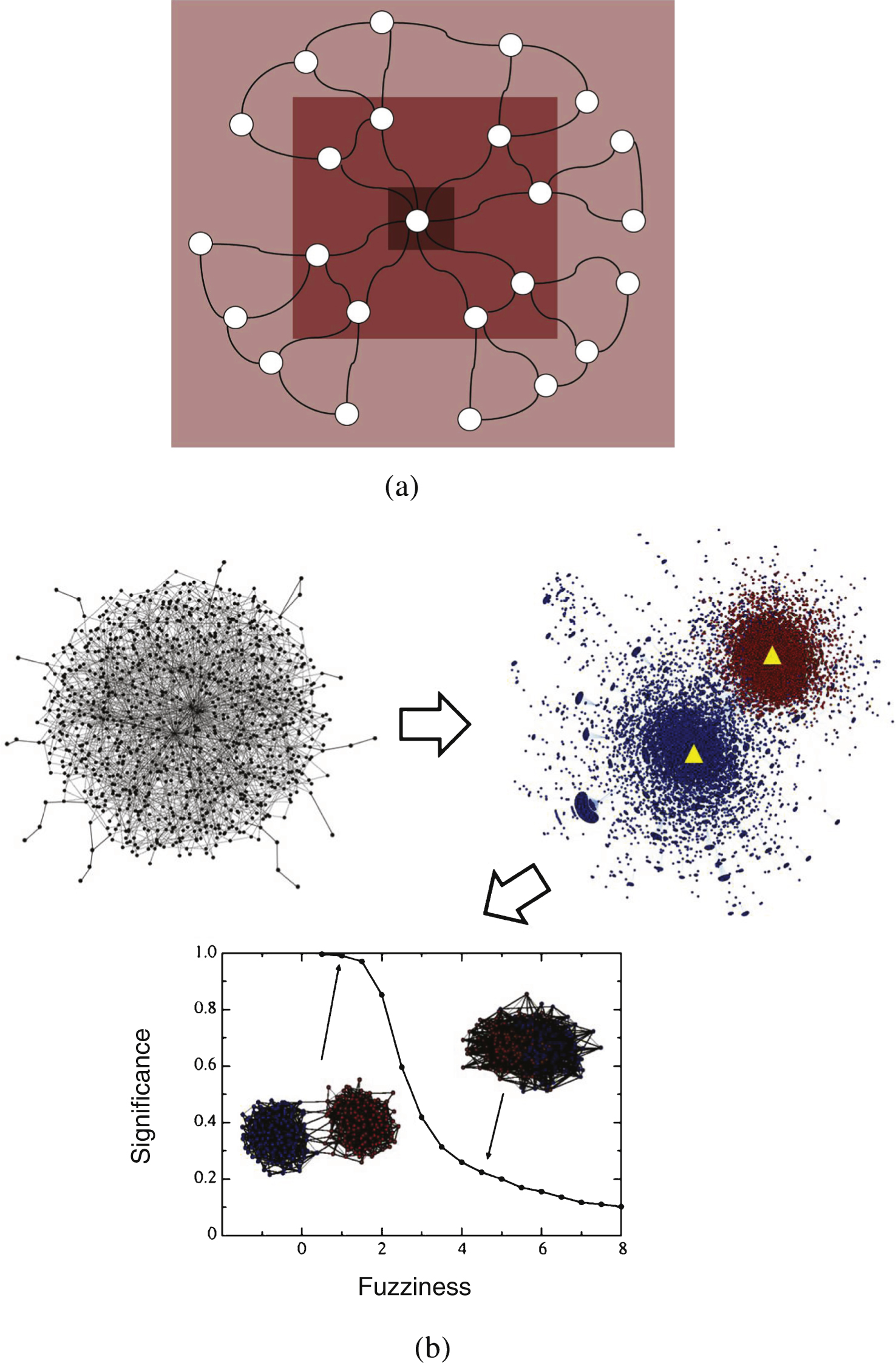
Fig.2
(a) The network topology of Zachary karate network. Two communities are represented by different shapes and colors. Node 1 and 34 are leaders which highlighted in the origin graph. (b) In every circle, sectors with different colors represent different communities. It can be noticed that the community partition in the rightmost circle is strongest due to the fewest intercommunity edges. When we use a given optimization method to evolve the community configure X (describe by different sectors) based on maximizing the objective function max Q = f (X), the significance of X also evolves correspondingly. The F score is utilized to measure the significance of community configure X. Here, the global maximum of F is maybe an asymptotically stable fixed point of dynamical system associates to community configure X in the rightmost circle.
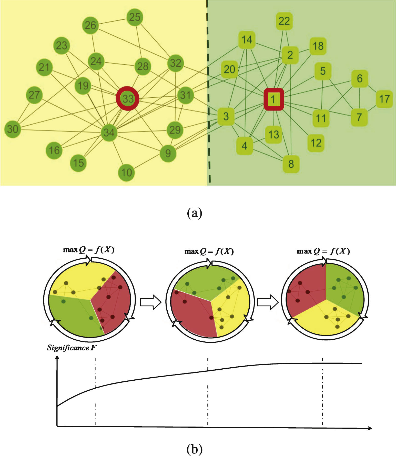
Fig.3
The experimental results of significance 〈F〉 on GN benchmark network and each point in curves is obtained by testing 100 times. (a) For all five optimization methods, 〈F〉 decreases with increasing of 〈k out 〉. For a given network, when 〈F〉 is larger than 0.3 on average(〈k out 〉≈4), one can say there exit significant community structure. (b)The value of 〈F〉 corresponding to μ = 0.3 will be larger than μ = 0.1 for the Hofman & Wiggins method and Label propagation method. This implies as the width parameter μ increases, the significance favors tighter communities with fewer elements.
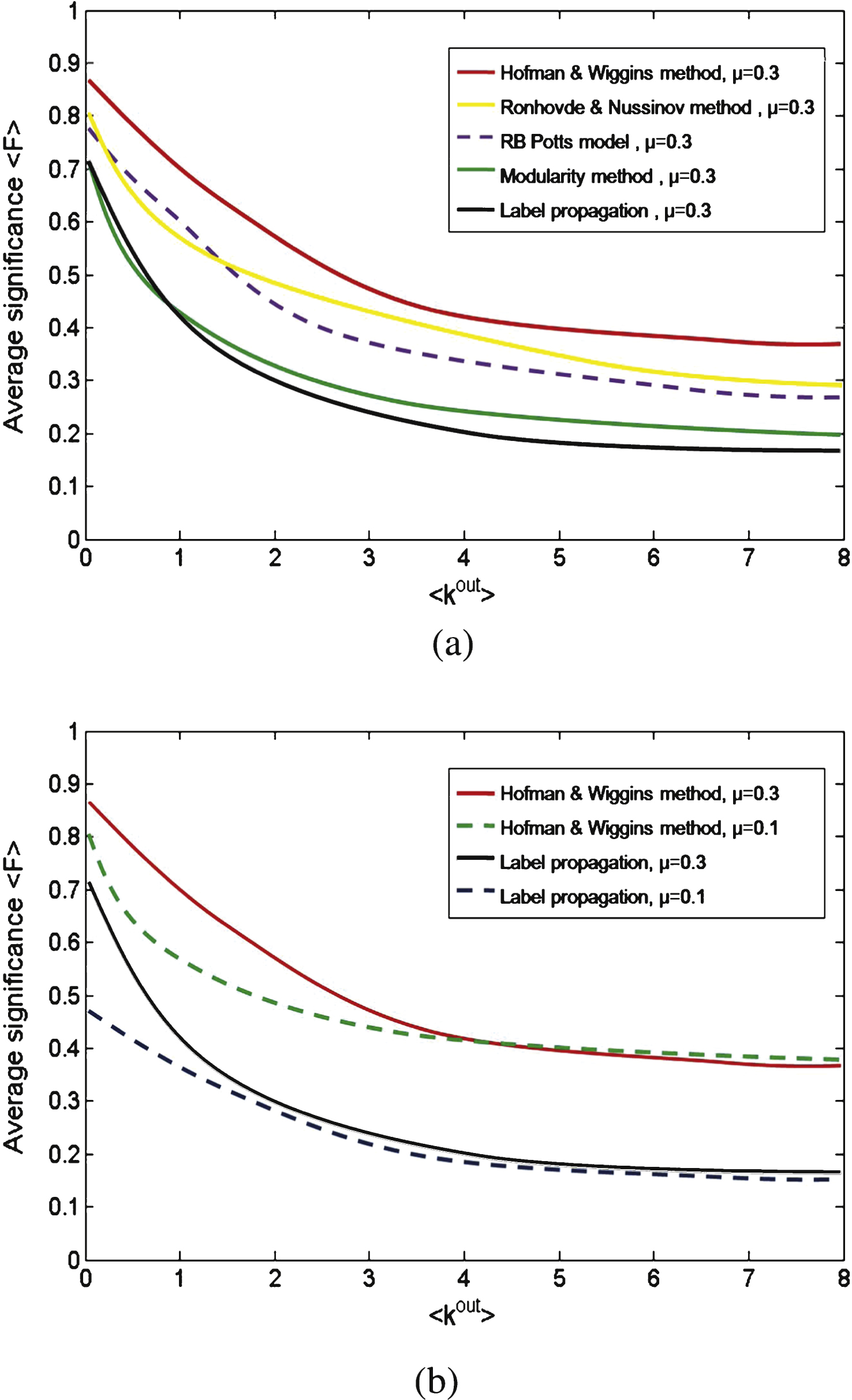
Fig.4
The performance of significance 〈F〉 on LFR benchmark network and each point in curves is obtained by testing 100 times. (a) In this network, the average degree k = 20, maximum degree is 50 and P (k) ∝ k γ . Maximum and minimum community sizes are 50 and 20 respectively. For all five algorithms, the 〈F〉 index decreases with the increasing of mix parameter θ. When θ ≥ 0.5 on average (no significant community), 〈F〉 is near 0.3 which is similar with GN network. (b) The value of 〈F〉 corresponding to μ = 0.3 will be larger than μ = 0.1 for the Hofman & Wiggins method and Label propagation method.
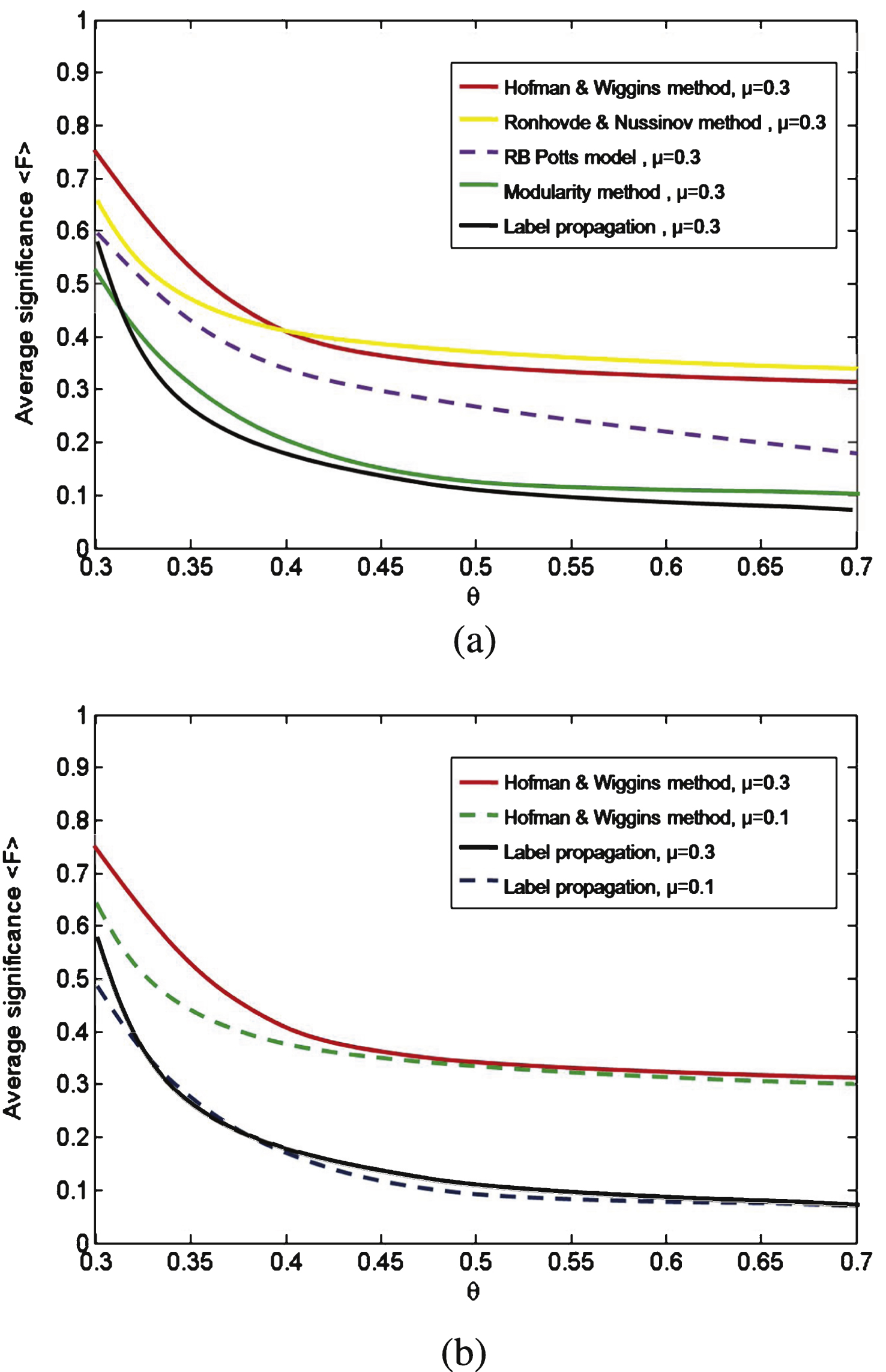
Fig.5
The performance of social significance 〈F〉 on stochastic block model. In this example, there are N = 5000 nodes and q = 10 groups. The average degree c = 8 and parameter ɛ = c out /c in is used to control the fuzziness of generated network. Each point in curves is obtained by testing 100 times. With the increasing of ɛ, the 〈F〉 index decreases. For all algorithm, when the corresponding 〈F〉 is nearly larger than 0.3 on average (ɛ ≈ 0.4), there exists significant community structure which may detectable.
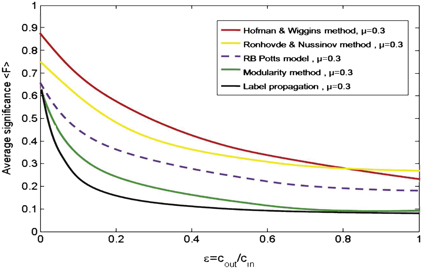
Table 1
Comparison of various algorithms with 〈F〉 values
| Networks | Algorithms | Values of 〈F〉 |
| Zachary | Label | 0.641 |
| GN | 0.735 | |
| RB Potts | 0.827 | |
| Collage football | Label | 0.602 |
| GN | 0.758 | |
| RB Potts | 0.831 | |
| Political books | Label | 0.581 |
| GN | 0.698 | |
| RB Potts | 0.717 |


