
Discrete Wavelet Transform based ECG classification using gcForest: A deep ensemble method
Abstract
BACKGROUND:
Cardiovascular diseases (CVDs) are the leading global cause of mortality, necessitating advanced diagnostic tools for early detection. The electrocardiogram (ECG) is pivotal in diagnosing cardiac abnormalities due to its non-invasive nature.
OBJECTIVE:
This study aims to propose a novel approach for ECG signal classification, addressing the challenges posed by the complexity of ECG signals associated with various diseases.
METHODS:
Our method integrates Discrete Wavelet Transform (DWT) for feature extraction, capturing salient features of cardiovascular diseases. Subsequently, the gcForest model is employed for efficient classification. The approach is tested on the MIT-BIH Arrhythmia Database.
RESULTS:
The proposed method demonstrates promising results on the MIT-BIH Arrhythmia Database, achieving a test accuracy of 98.55%, recall of 98.48%, precision of 98.44%, and an F1 score of 98.46%. Additionally, the model exhibits robustness and low sensitivity to hyper-parameters.
CONCLUSION:
The combined use of DWT and the gcForest model proves effective in ECG signal classification, showcasing high accuracy and reliability. This approach holds potential for improving early detection of cardiovascular diseases, contributing to enhanced cardiac healthcare.
1.Introduction
In modern society, cardiovascular diseases (CVDs) such as heart failure and myocardial infarction have been the leading causes of death globally [1]. As electrocardiogram (ECG) can reflect the electrical activities of heart, meanwhile, is a non-invasive technique, and it has been widely used in detecting and diagnosing cardiovascular abnormalities. However, the ECG signals of many diseases are complex and challenging to identify, causing a growing demand for ECG classification with high accuracy and high reliability [2].
Several methods have been proposed to classify ECG signals and detect abnormalities. In traditional machine learning, researchers utilize Hermit polynomial features [3], Hjorth descriptor and Principal component analysis (PCA), etc. to extract the features of ECG signals. Meanwhile, Support Vector Machine (SVM), Random Forest (RF), Decision Tree (DT), etc. are used in classification. On the other hand, deep learning methods are utilized in this field, such as Long Short-Term Memory (LSTM) and Convolutional Neural Networks (CNN).
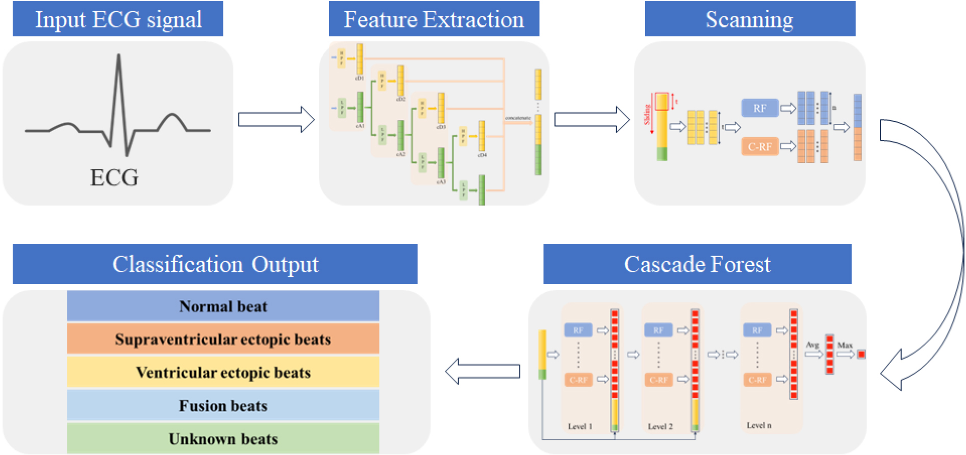
In this paper, we introduce a novel and effective method for ECG signal classification. Utilizing the Discrete Wavelet Transform (DWT), we extract the salient features indicative of cardiovascular diseases. Subsequently, we use the gcForest model, initially introduced by Zhi-Hua Zhou et al. [4] in 2017 to attain optimal classification outcomes. The method we developed has been trained and assessed using the MIT-BIH Arrhythmia Database [5], demonstrating a high accuracy of 98.55% on the test set. The overall process of our proposed model is shown in Fig. 1.
Figure 1.
Overall process of the DWT-gcforest model.
2.Dataset
For the evaluation of our proposed method’s performance, the MIT-BIH Arrhythmia Database was utilized in this research. The MIT-BIH Arrhythmia Database serves as the inaugural standard benchmark for evaluating arrhythmia detectors and has been utilized both for detector assessment and fundamental cardiac research. The dataset is available at PhysioNet and it consists of 48 types of recordings. Each recording is sampled at 360 Hz with a 30-minute duration and it has an annotation file which is identified by experts. Meanwhile, the classification of arrhythmia types is delineated by the American Association of Medical Instrumentation (AAMI), providing a structured framework for categorization. In this context, we concentrate solely on the five pivotal arrhythmia groups sourced from the MIT-BIH database, as delineated in Table 1.
Table 1
Five major groups in the MIT-BIH Arrhythmia Database
| Group | Class |
|---|---|
| N | Normal beat |
| Atrial escape beat | |
| Nodal premature escape beat | |
| Left bundle brunch block beat | |
| Right bundle brunch block beat | |
| F | Fusion of ventricular and normal beat |
| S | Supra-ventricular premature beat |
| Atrial premature beat | |
| Nodal premature beat | |
| Aberrated atrial premature beat | |
| V | Ventricular escape beat |
| Premature ventricular contraction beat | |
| Q | Paced beat |
| Unclassifiable | |
| Fusion of paced and normal beat |
3.Methodology
In this section, we present an in-depth overview of the feature extraction process utilizing Discrete Wavelet Transform (DWT) [6], along with the multi-class classification technique using gcForest. Meanwhile, a thorough exposition of the proposed model is presented.
3.1Discrete Wavelet Transform
Wavelet transform can comprehensively extract both the time-domain and frequency-domain characteristics of a signal, enabling a holistic representation of the original signal. Contrary to the Short Time Fourier Transform (STFT) [7] which analyzes signals at a fixed resolution, the wavelet transform is more adept at analyzing time-varying and non-stationary signals such as ECG. Consequently, numerous studies utilize wavelet transform techniques for feature extraction from ECG or denoising ECG signals.
Wavelet transform is categorized into Continuous Wavelet Transform (CWT) [8] and Discrete Wavelet Transform (DWT), serving as a fundamental tool in signal processing. In real-world EEG signal acquisition, signals are typically discrete. Moreover, the computational overhead of utilizing all wavelet coefficients by CWT is considerable. Thus, it is adequate to select a discrete subset of child wavelets to effectively reconstruct a signal from its corresponding wavelet coefficients. In this paper, we utilize the DWT method for feature extraction of ECG signals.
The wavelet transform theory is grounded on a function known as the mother wavelet
(1)
Child wavelets are dilated by a factor of a and shifted by a factor of b. In the discrete wavelet transform, we ensure that the pair (a, b) consists of discrete values, hence the corresponding wavelet is represented as:
(2)
Where
Given the discrete ECG signal
(3)
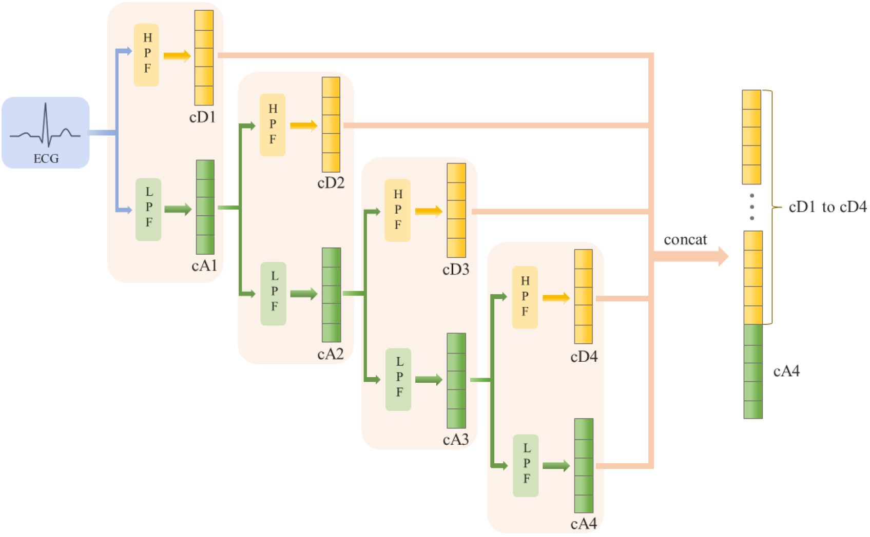
In practical applications, the fast Discrete Wavelet Transform (DWT) algorithm proposed by Mallat [9] is frequently utilized. This algorithm effectively decomposes an ECG signal into two distinct sub-bands: the low-frequency sub-bands, known as approximation coefficients (cA), and the high-frequency sub-bands, known as detail coefficients (cD). Moreover, fast DWT contains down-sampling by a factor of 2. When an origin signal passes through two filters, the signal is decomposed into a high-frequency component cD1 and a low-frequency component cA1. This process is termed as a decomposition of level 1. During the decomposition of level 2, cA1 is further decomposed into low-frequency component cA2 and high-frequency component cD2. Consequently, the outputs are cD1, cD2, and cA2. The decomposition formula is defined as follows:
(4)
Where
Figure 2.
Illustration of feature extraction structure.
3.2GcForest
The gcForest model was proposed by Zhi-Hua Zhou et al. [4] in 2017 as a collection of non-differentiable modules, characterizing an ensemble of ensembles approach that necessitates fewer hyper-parameters compared to deep neural networks. This implies a significant reduction in model complexity, which in turn lowers computational demands. Notably, the gcForest demonstrates commendable robustness concerning hyper-parameters. Moreover, the gcForest architecture incorporates a Cascade Forest structure for deriving the final classification and employs a procedure known as Multi-Grained Scanning to enhance the representation of data [10]. In this section, we will delineate both the Cascade Forest structure and the Multi-Grained Scanning mechanism.
3.2.1Cascade forest structure
Inspired by the processing of raw features in Deep Neural Networks, the gcForest model adopts a cascade structure to enhance its analytical capabilities. This structure is comprised of numerous layers, each of which constitutes an ensemble of decision tree forests. Since the gcForest model represents an ensemble of these layers, it is also referred to as an ensemble of ensembles. The structure is shown in Fig. 3.
Figure 3.
Structure of Cascade Forest (Suppose there are 5 classes).
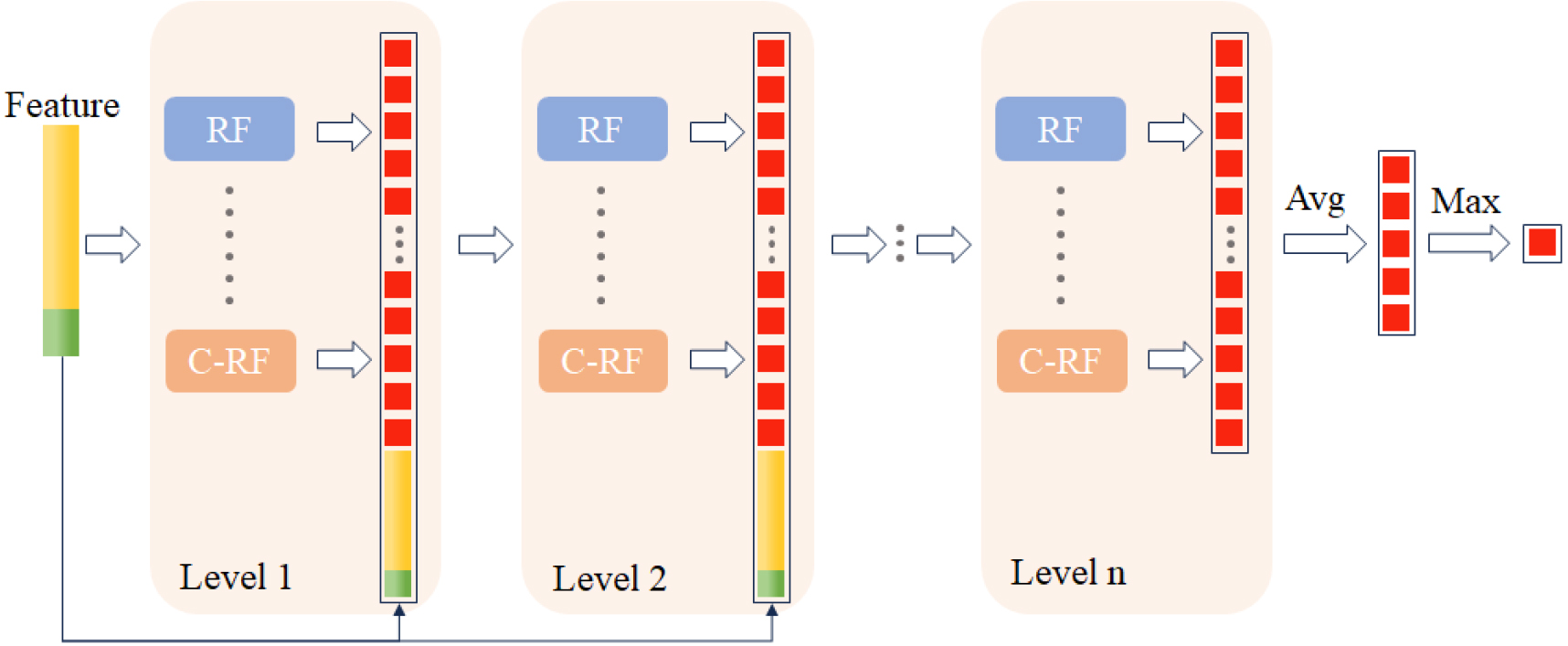
Each layer within this structure accepts data from the preceding layer and concatenates them with the original features before passing them on to the subsequent layer. In the construction of each layer, different types of forests are employed to amplify the diversity of the ensembles, which can contribute positively to the model’s performance. Typically, each layer contains two varieties of forests: random forest [11] and completely-random forest [12]. In the random forest, trees make splitting decisions by choosing the optimal feature with the best Gini index from a randomly selected subset of features. In contrast, trees within the completely-random forest select a feature at random to determine the splitting criterion. Lastly, it is important to note that each layer includes
In the gcForest framework, each forest evaluates an instance by calculating the class distribution. This is done by determining the proportion of training examples from different classes at the leaf node where the instance falls [4]. This method helps in estimating the likelihood of the instance belonging to each class based on the data observed in the training phase. Consequently, the class distribution vector is obtained by averaging the results across all trees within the same forest. Following the acquisition of the class distribution vector, it is concatenated with the original feature set to serve as the input for the subsequent level of the cascade. Assuming that the length of the input feature is
3.2.2Multi-Grained Scanning structure
To enhance the representation of the original data, a structure known as Multi-Grained Scanning is introduced to process the raw data before feeding it into the cascade forest structure [4]. The raw features are scanned with sliding windows of size
Figure 4.
Structure of scanning (the original input length is N).
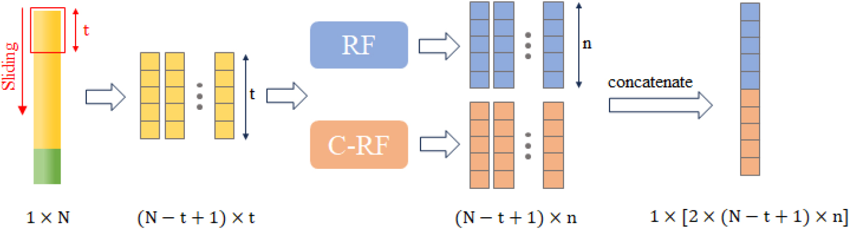
To enhance the randomness of data input, the scanning procedure employs multiple scans with different window sizes, a method known as Multi-Grained Scanning. This technique inputs features scanned with various window sizes into different cascade forests. The final results obtained from these forests are then aggregated. This multi-faceted approach allows for a more robust and comprehensive feature representation by capturing the inherent patterns in the data at different scales, ultimately contributing to the versatility of the model.
3.3DWT-cascade forest architecture
The structure for feature extraction, employing Discrete Wavelet Transform (DWT), and ECG multi-classification, using gcForest, is detailed in Fig. 5. During the DWT-based feature extraction, we utilize a Daubechies-4 (db4) [13] wavelet filter bank and set the decomposition level to four. Each level of decomposition yields both approximation coefficients (cA) and detail coefficients (cD), with the decomposition input for the next level being the cA from the previous one. The length of cA and cD obtained at each level is the same, equal to
Figure 5.
DWT-based gcforest structure.
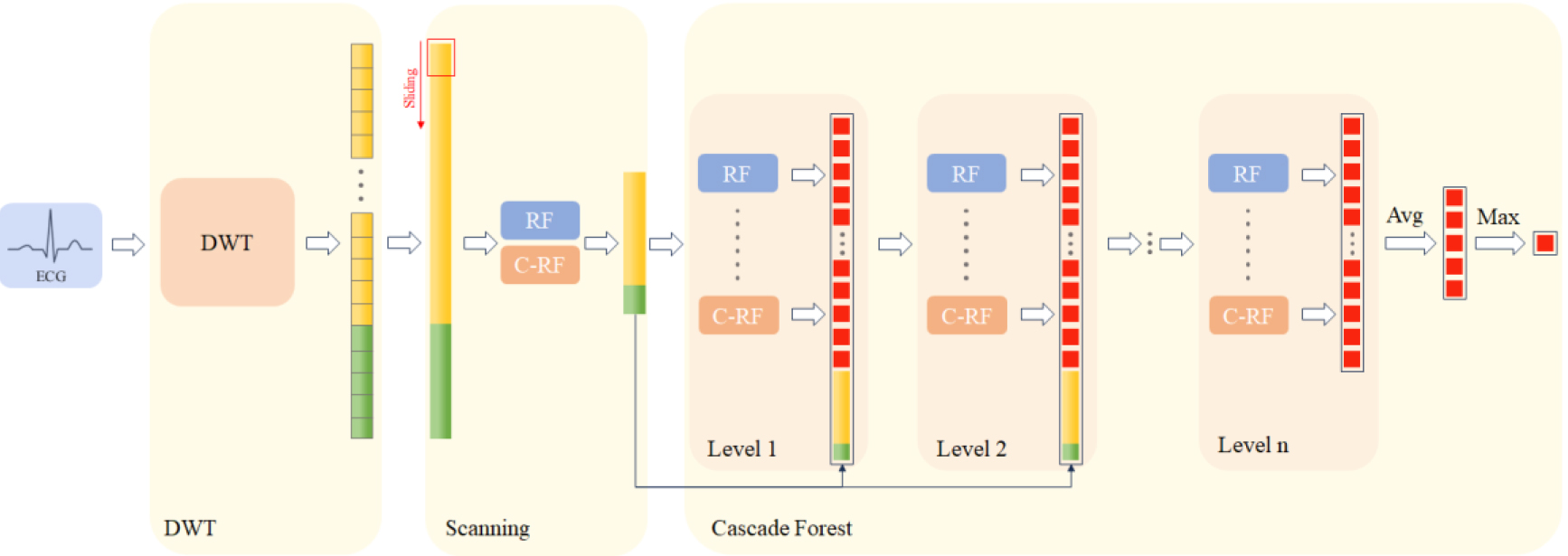
Subsequently, the features of length
4.Experiment
4.1Experimental setup
In order to evaluate our proposed model, we have partitioned the dataset into a training set and a test set, allocating 80% for training and 20% for testing. Meanwhile, we evaluate the performance of classification with the following metrics, which are defined by the following formula:
(5)
(6)
(7)
(8)
where FP denotes the False Positive, FN denotes the False Negative, TP denotes the True Positive and the TN denotes the True Negative.
In each layer of the gcForest, there are two hyper-parameters subject to fine-tuning: the number of forests (denoted as
Figure 6.
Performance with the change of the number of forests in each layer.
Figure 7.
Performance with the change of the number of trees in each forest.
4.2Result and discussion
The classification performance on the test set with the change of the number of forests within each layer and the number of trees within each forest is shown in Figs 7 and 7, respectively.
From Fig. 7, it can be discerned that variations in the number of forests in each layer yield disparities in the maximal and minimal values of accuracy, recall, precision, and F1, with differences approximately around 0.07%, 0.08%, 0.08%, and 0.08%, respectively. Similarly, Fig. 7 shows that by varying the number of trees in each forest, the difference between maximal and minimal values of accuracy, recall, precision, and F1 is approximately 0.06%, 0.06%, 0.09%, and 0.10%, respectively. Hence, to balance computational expenditure with model performance, we elect to set and as the final hyper-parameter configuration. In this setting, the model performance is characterized by an accuracy of 98.55%, recall of 98.48%, precision of 98.44%, and an F1 of 98.46%.
To appraise the performance of our proposed model more thoroughly, we have conducted a comparative analysis with existing methods. This includes traditional machine learning algorithms including LDA-MLP [14], SVM [15], XGBoost [16], and RandomForest [17], as well as deep learning methods comprising CNN [18], ResNet [19], DCNN [20], CNN-BiLSTM [21], and Deep Attention BiLSTM [22]. The outcomes of this comparison are delineated in Table 2.
Table 2
Comparison performance
| Method | Accuracy | Recall | Precision | F1 |
|---|---|---|---|---|
| LDA-MLP | 89.02% | 69.53% | 56.27% | 62.20% |
| SVM | 86.55% | 58.65% | 53.40% | 55.90% |
| XGBoost | 91.87% | 75.09% | 61.80% | 67.80% |
| Random forest | 94.60% | – | – | – |
| CNN | 94.03% | 73.48% | 57.00% | 64.20% |
| ResNet | 98.00% | – | – | – |
| DCNN | 91.33% | – | – | – |
| CNN-BiLSTM | 96.77% | 74.67% | 81.20% | 77.80% |
| Deep Attention BiLSTM | 96.72% | 96.43% | 96.51% | 96.46% |
| DWT | 98.55% | 98.48% | 98.44% | 98.46% |
Table 3
Ablation study result
| Method | Accuracy | Recall | Precision | F1 |
|---|---|---|---|---|
| gcForest | 98.29% | 98.23% | 98.29% | 98.25% |
| DWT | 98.55% | 98.48% | 98.44% | 98.46% |
In traditional machine learning algorithms, the LDA-MLP method [14] employs the forward floating search (SFFS) algorithm to derive a feature set, achieving an accuracy of 89.02%, a recall of 69.53%, a precision of 56.27%, and an F1-score of 62.20% on the dataset. The SVM classifier with Morphological and Dynamic Features [15] reached an accuracy of 86.55%. An ECG classification approach based on XGBoost [16] attained an accuracy of 91.87%. Finally, the Random Forest classifier with features utilizing wavelet packet decomposition [17] achieved the highest accuracy among machine learning algorithms, namely 94.60%.
In the domain of deep learning algorithms, a CNN [18] that directly uses raw signals as input achieved an accuracy of 94.03%, a recall of 73.48%, a precision of 57.00%, and an F1-score of 64.20%. A transfer learning method employing ResNet [19] reached an accuracy of 98.00%. A DCNN with raw ECG signals for inputs [20] obtained an accuracy of 91.33%. The CNN-BiLSTM [21] and Deep Attention BiLSTM [22], both ECG classification methods based on CNN and LSTM, differ in that the latter incorporates an attention mechanism. They achieved accuracies of 96.77% and 96.72%, respectively. Lastly, the deep ensemble method proposed in this paper demonstrated optimal performance, achieving an accuracy of 98.55%, a recall of 98.48%, a precision of 98.44%, and an F1-score of 98.46%.
4.3Ablation study
To evaluate the contribution of the DWT-based feature extraction module, we conduct an ablation study on the proposed model. We only remove the feature extraction module from the proposed model, while the overall hyper-parameter settings remain the same. As shown in Table 3, while the multi-grained scanning structure is capable of enhancing the representation of the original data, the DWT-based feature extraction module improves the performance of the proposed model.
5.Conclusions
In this paper, we propose a DWT-gcforest method for ECG signal classification with lower computational costs. Discrete wavelet transform (DWT) is utilized to extract the feature representation of the original ECG signal, while the Multi-Grained Scanning structure enhances the representation. With the structure of Cascade Forest, we obtain the classification outputs. Meanwhile, comparative experiments and ablation studies on the model were conducted using the MIT-BIH Arrhythmia Database. The classification outcomes of the model manifested as an accuracy of 98.55%, a recall of 98.48%, a precision of 98.44%, and an F1 of 98.46%. The results from our experiments demonstrate that the model we proposed surpasses other models in performance. Moreover, our model demonstrates insensitivity to hyper-parameters. Ablation studies have shown that the feature extraction module based on the DWT has improved the model’s performance. However, a current limitation of the gcforest algorithm is its exclusive reliance on CPU-based computation, which considerably slows down the processing speed. Additionally, the algorithm proposed in this paper is based on intra-patient classification and does not account for the potential performance in inter-patient classification scenarios. In the future, we intend to explore different methods for feature extraction to enhance the model’s performance and reduce computational complexity. Additionally, we will investigate inter-patient ECG classification to broaden the scope and applicability of our research.
Acknowledgments
This work was supported by the Fujian Provincial Health and Middle-aged Youth Backbone Talent Training Project (2022GGB017).
Conflict of interest
The authors have no conflicts of interest to declare.
References
[1] | Moraga P. GBD 2016 Causes of Death Collaborators Global, regional, and national age-sex specific mortality for 264 causes of death, 1980–2016: A systematic analysis for the Global Burden of Disease Study 2016. Lancet. (2017) ; 390: (10100): 1151-1210. |
[2] | Chung CT, Lee S, King E, et al. Clinical significance, challenges and limitations in using artificial intelligence for electrocardiography-based diagnosis. International Journal of Arrhythmia. (2022) ; 23: (1): 24. |
[3] | Ebrahimzadeh A, Ahmadi M, Safarnejad M. Classification of ECG signals using Hermite functions and MLP neural networks. Journal of AI and Data Mining. (2016) ; 4: (1): 55-65. |
[4] | Zhou ZH, Feng J. Deep forest. National Science Review. (2019) ; 6: (1): 74-86. |
[5] | Goldberger A, Amaral L, Glass L, Hausdorff J, Ivanov PC, Mark R, Stanley HE. PhysioBank, PhysioToolkit, and PhysioNet: Components of a new research resource for complex physiologic signals. Circulation [Online]. (2000) ; 101: (23): e215-e220. |
[6] | Zhang D, Zhang D. Wavelet transform. Fundamentals of image data mining: Analysis, Features, Classification and Retrieval. (2019) ; 35-44. |
[7] | Griffin D, Lim J. Signal estimation from modified short-time Fourier transform. IEEE Transactions on Acoustics, Speech, and Signal Processing. (1984) ; 32: (2): 236-243. |
[8] | Aguiar-Conraria L, Soares MJ. The continuous wavelet transform: A primer. NIPE-Universidade do Minho. (2011) . |
[9] | Mallat SG. A theory for multiresolution signal decomposition: The wavelet representation. IEEE Transactions on Pattern Analysis and Machine Intelligence. (1989) ; 11: (7): 674-693. |
[10] | Utkin LV, Kovalev MS, Meldo AA. A deep forest classifier with weights of class probability distribution subsets. Knowledge-Based Systems. (2019) ; 173: : 15-27. |
[11] | Breiman L. Random forests. Machine Learning. (2001) ; 45: : 5-32. |
[12] | Liu FT, Ting KM, Yu Y, et al. Spectrum of variable-random trees. Journal of Artificial Intelligence Research. (2008) ; 32: : 355-384. |
[13] | Vonesch C, Blu T, Unser M. Generalized Daubechies wavelet families. IEEE Transactions on Signal Processing. (2007) ; 55: (9): 4415-4429. |
[14] | Mar T, Zaunseder S, Martínez JP, et al. Optimization of ECG classification by means of feature selection. IEEE Transactions on Biomedical Engineering. (2011) ; 58: (8): 2168-2177. |
[15] | Ye C, Kumar BVKV, Coimbra MT. Heartbeat classification using morphological and dynamic features of ECG signals. IEEE Transactions on Biomedical Engineering. (2012) ; 59: (10): 2930-2941. |
[16] | Shi H, Wang H, Huang Y, et al. A hierarchical method based on weighted extreme gradient boosting in ECG heartbeat classification. Computer Methods and Programs in Biomedicine. (2019) ; 171: : 1-10. |
[17] | Li T, Zhou M. ECG classification using wavelet packet entropy and random forests. Entropy. (2016) ; 18: (8): 285. |
[18] | Sellami A, Hwang H. A robust deep convolutional neural network with batch-weighted loss for heartbeat classification. Expert Systems with Applications. (2019) ; 122: : 75-84. |
[19] | Islam R, Rahman M, Ismail SM, et al. Transfer Learning in Deep Neural Network Model of ECG Signal Classification. 2022 International Conference on Recent Progresses in Science, Engineering and Technology (ICRPSET). IEEE. (2022) . pp. 1-4. |
[20] | Yildirim O, San Tan R, Acharya UR. An efficient compression of ECG signals using deep convolutional autoencoders. Cognitive Systems Research. (2018) ; 52: : 198-211. |
[21] | Chen A, Wang F, Liu W, et al. Multi-information fusion neural networks for arrhythmia automatic detection. Computer Methods and Programs in Biomedicine. (2020) ; 193: : 105479. |
[22] | Tao Y, Li Z, Gu C, et al. ECG-based expert-knowledge attention network to tachyarrhythmia recognition. Biomedical Signal Processing and Control. (2022) ; 76: : 103649. |


