Enhanced acrylic gauge with five eccentric circles for optimizing CT angiography spatial resolution via Taguchi’s methodology

2.1Taguchi’s analysis

Robust and convenient optimization of a single demanded quality is provided by Taguchi’s analysis, implying the integration of multiple factor contributions into the unique orthogonal array. Thus, only limited practical measurements are summarized, while the particular assigned factor contribution is easily distinguished from those of other factors and the background noise. The key influencing factors of the main performance are assessed via the analysis of variance (ANOVA). The optimal combinations of such factors for the CTA scan protocol are identified via the signal-to-noise ratio (S/N). More detail can be found elsewhere [13, 14, 15].

2.2Orthogonal arrays

Unlike other optimized methods, Taguchi analysis assures an optimal level of a specific factor from a finite preset of empirical data and those factors that affect the target. This study selected the following six factors of the CTA scan protocol: (A) kVp, (B) mAs, (C) scan pitch, (D) FOV, (E) gantry rotation time, and (F) reconstruction filter. Each factor was assigned to two or three levels, yielding a total number of 486 (2 × 3 × 3 × 3 × 3 × 3) combinations. Eighteen groups’ organization of measured data was performed via Taguchi’s approach, with data collection focused on grasping effects at the same confidence level as the conventional analysis of process optimization [13]. Taguchi’s standard L₁₈ (2¹× 3⁵) orthogonal array is presented in Table 1. Each column’s digits correspond to the practical arrangement or specific levels of particular factors (A–F). Table 2 depicts the six factors (A–F) as (A) kVp, (B) mAs, (C) scan pitch, (D) FOV, (E) gantry rotation time, and (F) reconstruction filter.

2.3Eccentric circles’ gauge and head phantom

To satisfy the quantified criteria of Taguchi’s recommendation, a unique head phantom with five eccentric circles’ gauge was customized according to the ICRU-48 report [16]. Figure 1(A) shows the designation chart of the special slice of the head phantom. Note that the depth of the curved slit was 0.8 mm (@loose region) and then gradually decreased to only 0.2 mm (@concise region) toward the brain edge. This was designed to simulate the real brain tissue since the gap between each circle in the concise region was very compact and assigned to simulate the microvasculature inside the brain, so it not only had a very narrow width but also had a very thin depth (B) the close-up view of the eccentric circles gauge, as shown, there are five eccentric circles of 0.5 mm slit with various radii of 2.75, 5.25, 7.75. 10.25, and 12.75 mm, respectively, and each circle’s center deviates from the last center by 1.50 mm to make the eccentric effect. Then, the gap among every circle has different widths, as shown in (C) 20^∘ or 30^∘ and (D) 90^∘, 135^∘ (90 + 45 = 135), or 180^∘. For instance, the gap width was 1.4872, 1.5242, 0.5949, 1.7812, and 2.7500 mm at a 90^∘ angle of profile and measured from top to bottom. In addition, the gap width among all the circles at 0^∘ and 18^∘ equaled 0.5000 and 3.5000 mm, respectively (cf. Fig. 1(C) and (D)). Any angle of the profile could be intercepted to offer five continuous peaks with various distances among those, and it offered a flexible gap width from 0.5 mm at 0^∘ to 3.50 mm at 180^∘ on a very precise scale for surveying the CTA spatial resolution.

Figure 1.

(A) The designation chart of the special slice of the head phantom. Note that the depth of the curved slit was 0.8 mm (@loose region) and then gradually decreased to only 0.2 mm (@concise region) toward the brain edge. (B) Close-up view of the eccentric circle gauge. As shown, there are five eccentric circles of the 0.5 mm slit with various radii of 2.75, 5.25, 7.75. 10.25 and 12.75 mm, respectively, and each circle’s center deviates from the last center by 1.50 mm to make the eccentric effect. Then, the gap among every circle has different widths, as shown in (C) 200 or 300 and (D) 900, 1350 (90 + 45 = 135), or 1800.

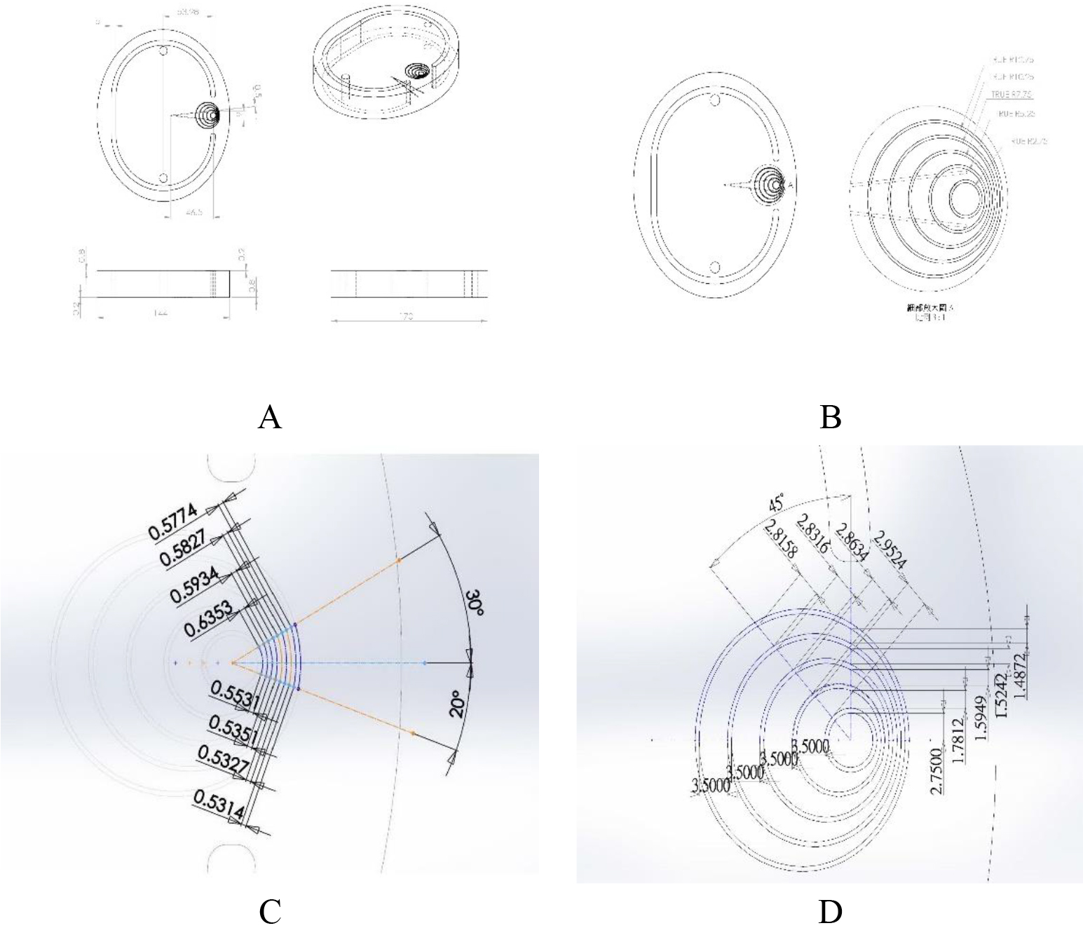
Figure 2.

(A) The customized acrylic layer of the head phantom, (B) the real image from the CTA scan, (C) the head phantom was assembled by seven similar acrylic layers, (D) the assembled head phantom was installed in the proper position with stand and ready for CTA scan.

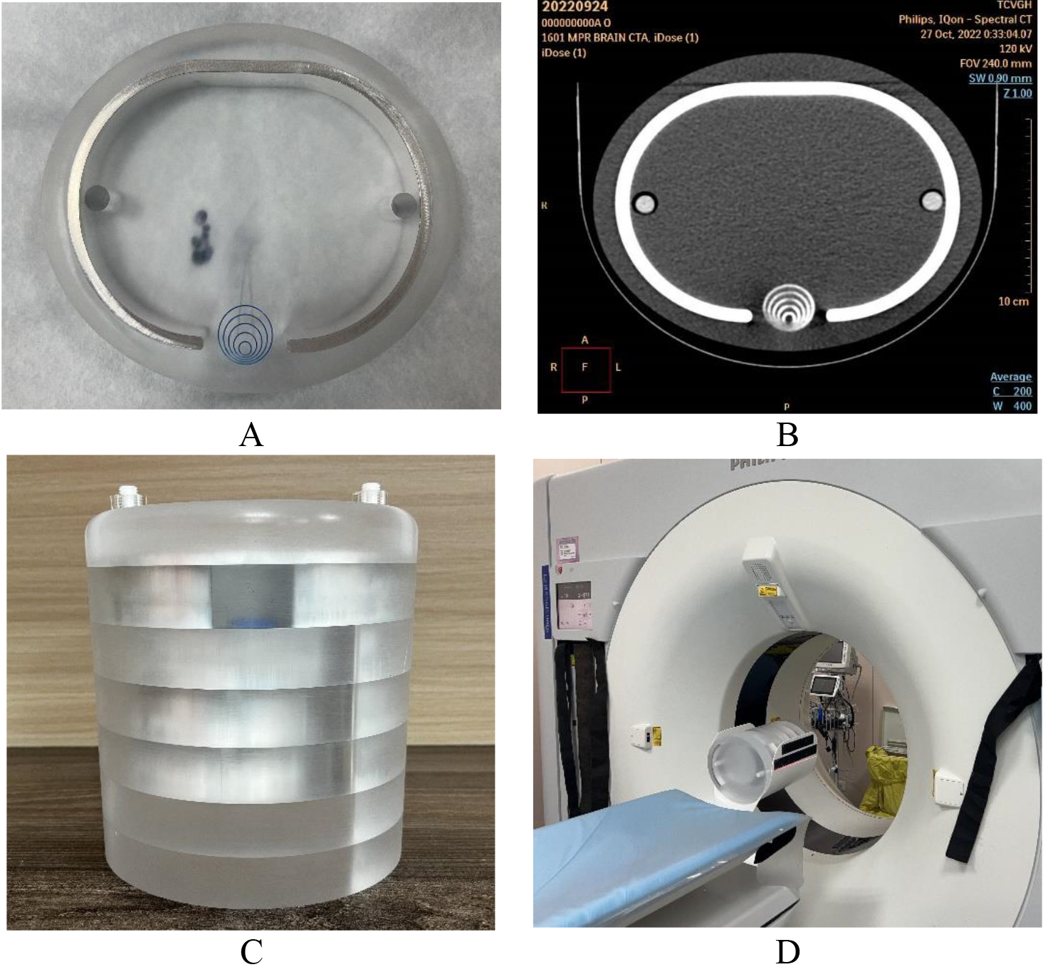
Figure 2(A) implies the customized acrylic layer of the head phantom. The eccentric circle gauge was drilled by precision milling machining, (B) the real image from the CTA scan. Seventy percent of the contrast media solution (Xenetix^® 350) was injected along the slit to intensify the contrast difference in the CTA scan. In addition, the CT number of brain soft tissue and artery was 20–60 and 200–500 HU, respectively, whereas the CT number of this phantom was 100 and 280–510, respectively, in the real scan. (C) Seven similar acrylic layers assembled the head phantom, and each had a different head shell profile made of aluminum, according to the ICRU-48 report [16]. (D) The assembled head phantom was installed properly with a stand and ready for the CTA scan.

2.4Imaging ranking and signal-to-noise ratio

Using Taguchi’s orthogonal array, 18 scans of five eccentric circles’ gauge imaging qualities [cf. Tables 1 and 2] were obtained and submitted to three well-trained radiologists for their ranking by the double-blinded procedure in three discrete periods to ensure reproducibility. Judging by contrast, sharpness, or spatial resolution, they ranked the imaging quality from 1 (the worst) to 18 (the best) among the 18 groups under study. Their scores were averaged to derive the S/N ratio as in [17]:

where std and Avg are the standard deviation and the average of 9 (3 × 3) ranked scores in each group. Smaller std values and larger Avg ones being favorable for the quality, a combination with a high average and low deviation would rank the best.

2.5ANOVA test

The ANOVA test became an integral part of imaging quality optimization. The sums of the squared variance of factor and error (S⁢S𝑓𝑎𝑐𝑡𝑜𝑟 and S⁢S𝑒𝑟𝑟𝑜𝑟, respectively) were compared to rank the importance of individual factors [18], The dominant contribution of S⁢S𝑓𝑎𝑐𝑡𝑜𝑟 is crucial in the optimizing process, while minor factors are generally preset to avoid disturbing contributions from the dominant ones [19]. If a dominant factor has low std values in the statistical analysis, it is defined as a tune-up factor in the optimal process to eliminate the disturbance from systematic error. Although identifying the tune-up factor in best combinations is quite problematic, it is useful for adjusting the expected value without any additional disturbance of the standard deviation in measured data, thus reducing the S⁢S𝑒𝑟𝑟𝑜𝑟 value [20].

3.1Analysis of raw data

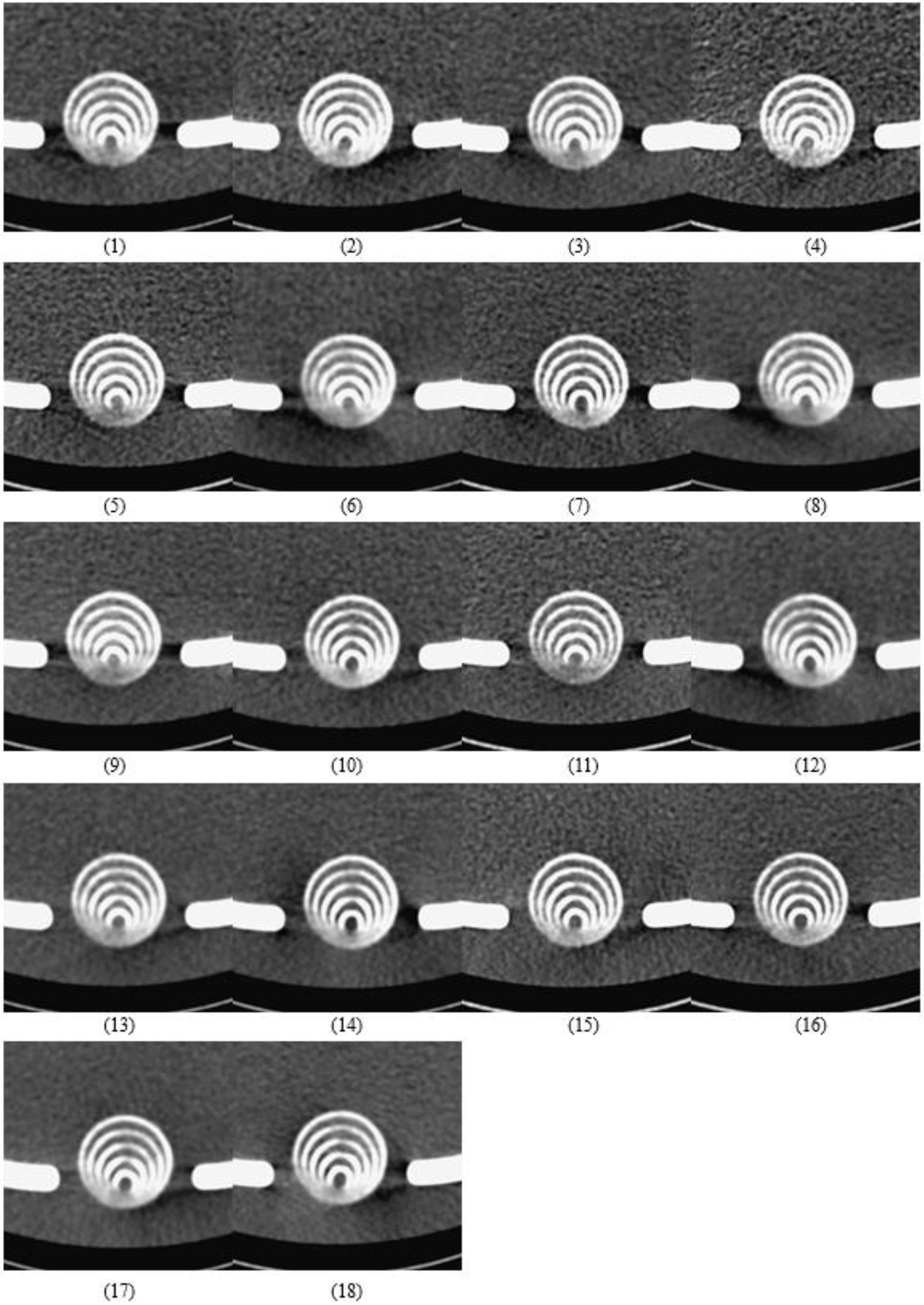
In total, 18 images were obtained via CTA scans, as shown in Fig. 3. As described in Section 2.4, their imaging quality was ranked by three radiologists. As shown in Table 3, 9 (3 × 3) ranked data for 18 combinations of six factors were averaged, and the S/N values were derived via Eq. (1). Accordingly, the fish-bone plots of each factor were constructed based on Taguchi’s L₁₈ orthogonal array [14, 15]. As seen in Fig. 4, the calculated values Avg, std, or S/N of five factors (except for A(kVp) indicated their prevailing performance in practical measurements, while the latter factor had a minor contribution to the optimization.

Figure 3.

The eighteen images from the real CTA scan. The imaging quality of 18 groups was ranked based on contrast, sharpness, or spatial resolution by three well-trained radiologists in three discrete periods to ensure reproducibility and suppress random error in the computation of the variance samples.

3.2ANOVA test

The raw ranked data of 18 groups were also included to proceed with ANOVA. As listed in Table 4, five factors had significant differences, except factor A (kVp), indicating that an optimal process was needed. Factor F (reconstruction filter) contributed most to the CTA scan for pursuing spatial resolution in reality. The extremely high contribution (64.47%) among all factors occupied over half the performance of spatial resolution for the CTA scan, whereas the second factor C (pitch) only had 4.82% to all. The specific other factors also had as many as 24.79%, indicating that there was still some intrinsic uncertainty beyond this survey that disturbed the performance of the CTA scan. In contrast, the low contribution from the error term (2.25%) denoted a negligible uncertainty from the random error. The three well-trained radiologists assigned in this study had excellent agreement on imaging quality; thus, the average std was as low as 2.48. In contrast, the theoretical std should be 9.5=3.08 to fulfill the normal distribution in reality.

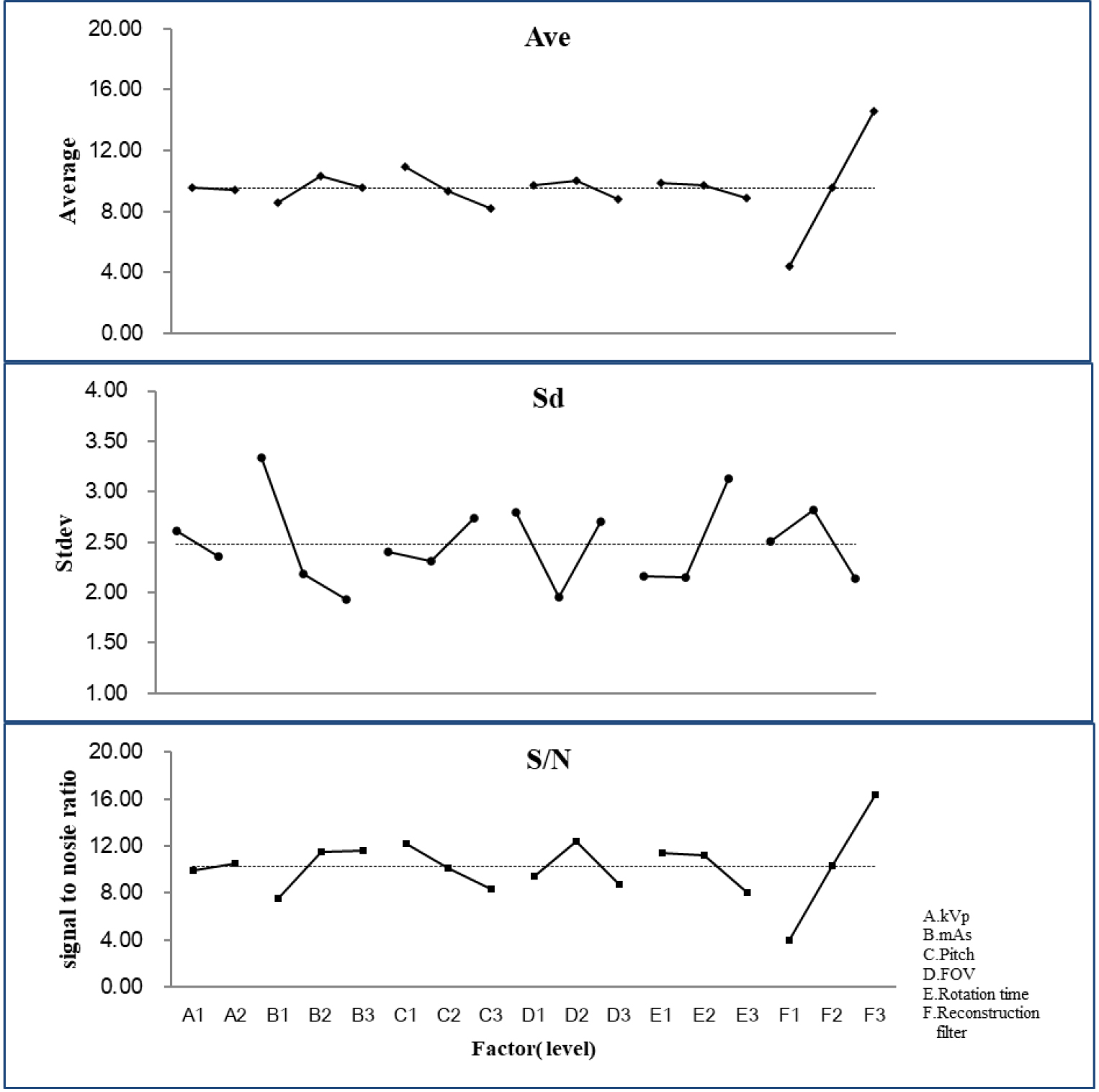
Figure 4.

Only factor A(kVp) played a minor contribution to the optimization since the calculated Avg, std, or S/N of the other five factors had prevailing performance in practical measurement.

4.1Semi-auto profile analysis of CTA scan imaging quality

To further quantify the spatial resolution of the five eccentric circles’ gauge, the minimal detectable difference (MDD) was introduced to precisely quantify the difference among various factor combinations of the CTA scan protocol. The MDD was defined in [9, 10, 11, 12] as follows:

where X1 and X2 are the centers of peaks 1 and 2, respectively, while FWHM is the full width at half maximum of the specific peak. To evaluate the four MDDs from two nearby peaks along the five gap slits, the valley edge of the two nearby peaks was changed gradually to provide the quantitative assessment of its edge width in its original designation. In addition, a small MDD is always preferable for the CTA scan image due to its superior recognizable capability in diagnosing the brain vessel structure. Accordingly, a numerical technique in MATLAB 2021b [21] and OriginPro 2017 [22] is integrated to analyze the MDD. In doing so, the CTA scan image of the eccentric circle gauge is converted from the original DICOM to a data matrix of 16 digits. Then, the default Poisson distribution program in OriginPro is run to automatically identify the peak center and FWHM of five peaks of the eccentric circle gauge. Such MDD assessment is easier than manual calculation via the conventional approach [9, 10, 11, 12]. Moreover, the MDD is recorded only if the four MDDs in the specific case pass the criteria (cf. Eq. (2)); thus, the reported MDD exceeds others obtained using a V-shaped slit since only one MDD is produced by two nearby peaks in the slice profile.

As illustrated in Fig. 5(A), the profile of the eccentric circle gauge from the CTA scan was converted from a gray image in DICOM format to an OriginPro data matrix of numerical digits and then analyzed by the default program to obtain the peak center and FWHM. (B) The original grayscale of eccentric circles in DICOM format (left) and redrawn data matrix from the OriginPro output (right). In addition, the conversion ratio (mm/channel) was derived from the real length divided by the digital channel in either the X- or Y-axis and equaled (24.53.04+27.83.38)/2=8.1 (mm/channel). The conversion ratio dominates the practical calculation of MDD in reality.

4.2Verifying the optimal setting

The optimal setting of the CTA scan can be verified by assembling the highest S/N of every factor; thus, the combination of factors should be A2, B3, C1, D2, E1, and F3 (cf. Fig. 4); in contrast, the highest S/N among the original eighteen groups is group 7 as A1, B3, C1, D2, E1, and F3 for comparison. Note that only factor A is changed from preset 120 to 100 kVp to reach the optimal result (cf. Table 2). In addition, the optimal combination of factors also extends beyond the original eighteen preset groups to obtain superior performance. The optimal recommendation derived from the L₁₈ orthogonal array can easily have an optimal suggestion beyond the original preset. In contrast, neither L₈ (2⁷) nor L₉ (3⁴) can have such capability to suggest the optimal setting beyond the preliminary realm in reality. The conventional preset factors were A2, B2, C2, D3, E1, and F2, which are the same as those listed in group 14 in this study (cf. Table 2).

Figure 6(I) shows the CTA scan imaging of the five eccentric circles’ gauges according to (A) the conventional preset, (B) the highest S/N (i.e., group 7 among 18 groups), or (C) the optimal preset. In addition, the 3D plot by OriginPro is also listed in Fig. 6(II) to emphasize the difference between the conventional and optimal CTA settings as (II-A) the conventional preset and (II-B) the optimal preset of the CTA factor combination. The optimal one shows clearer and sharper imaging quality in the 3D plot; however, the solid numerical evaluation of the spatial resolution still needs to be further quantified by MDD.

Figure 5.

(A) The profile of the eccentric circles’ gauge from the CTA scan was converted from a gray image in DICOM format to an OriginPro data matrix of numerical digits and then analyzed by the default program to obtain the peak center and FWHM. (B) The original grayscale of eccentric circles in DICOM format (left) and redrawn data matrix from the OriginPro output (right).

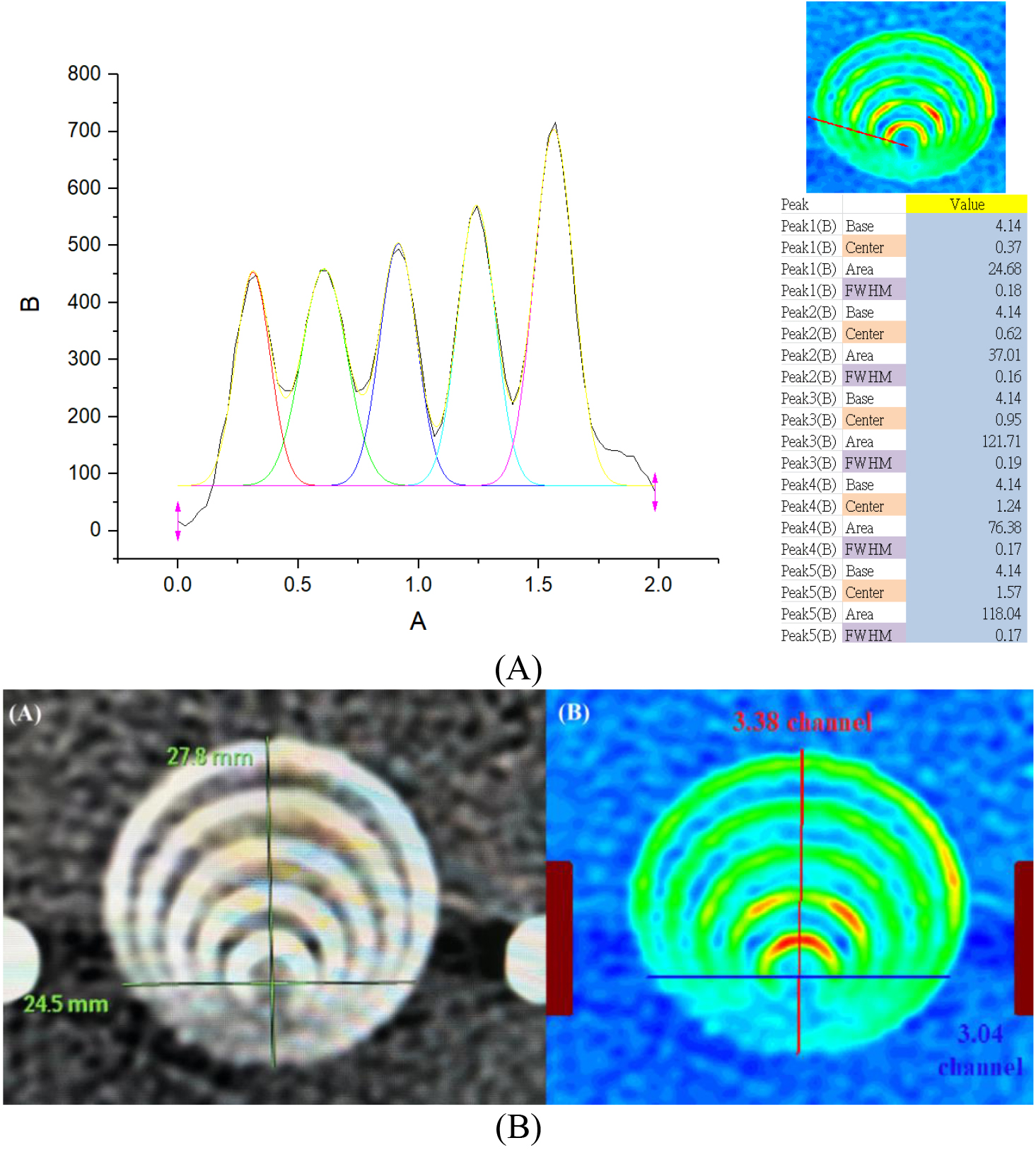
Figure 6.

(I) The CTA scan imaging of the five eccentric circles gauge according to (A) conventional preset, (B) the highest S/N (i.e., group 7 among 18 groups) or (C) the optimal preset, (II) 3D plot to emphasize the difference between conventional and optimal CTA setting as (II-A) the conventional preset and (II-B) the optimal preset of CTA factor combination.

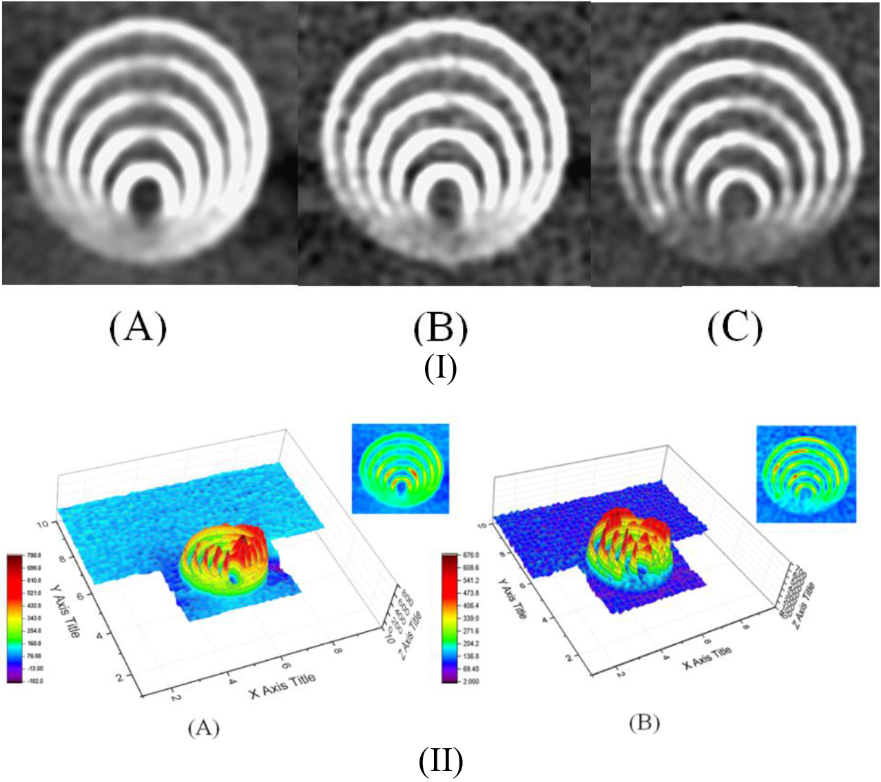
Table 5 shows the three combinations of various CTA factor settings. The minor difference in the CTA resetting eventually caused a significant difference in the imaging quality. It provided solid spatial resolution as precise as MDD of 0.01 mm.

4.3Validation by other quantified techniques

Figure 7.

The derived MTF 10% for (A) the conventional preset, (B) the highest S/N (i.e., group 7 among 18 groups), or (C) the optimal preset of the CTA factor combination is 4.732, 5.155, and 5.210 lp/cm, respectively, as analyzed by the CTA default program.

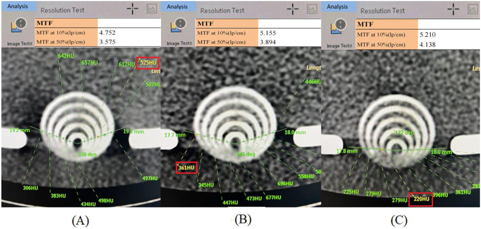
Many quantified techniques have been developed in CTA to evaluate spatial resolution. The modulation transfer function (MTF) [23] and signal-to-noise ratio (SNR) [24] are two major tools in quality assurance to ensure CTA spatial resolution. To precisely evaluate the spatial resolution, a line pair gauge is usually adopted in MTF to quantify the spatial resolution from a specific image’s change in light and darkness into the form of intensity and spatial frequency. Accordingly, MTF of 10% is recommended in radiation medical exposure quality assurance standard regulations as the basis for justifying high spatial resolution. As depicted in Fig. 7, the derived MTF 10% for (A) the conventional preset, (B) the highest S/N (i.e., group 7 among 18 groups), or (C) the optimal preset of the CTA factor combination is 4.732, 5.155, and 5.210 lp/cm, respectively, as analyzed by the CTA default program. Another analyzed index of CTA spatial resolution is SNR, which is defined as

where the CT value inside the specific ROI is divided by the standard deviation. A large SNR is always preferable to imply more useful information (signal) than unwanted data (noise). Thus, five 1 mm² ROIs were assigned separately from the ring of five eccentric circles, and the averaged SNRs with standard deviations were 7.95 ± 1.66, 8.36 ± 2.69 and 9.79 ± 2.53 dB for the conventional, highest S/N, and optimal preset CTA factor combinations, respectively. However, either MTF or SNR is calculated according to specific points; therefore, we have to assign many points (five points in this study) along the eccentric circles to derive the numerical data, whereas MDD is calculated based on a continuous profile to justify two near-by peaks being separated far enough to reach a 95% confidence level; thus, it is more reliable and convincible than others in reality.

4.4Comparing MDD obtained by various gauges in this and other studies

The MDD derived in this study was also compared to other. As depicted in Table 6, the MDD for either cardiac or mammography has a high spatial resolution, 016 or 0.09 mm. The mammography facility has Rh/Ag as the X-ray target and filter; thus, the soft X-ray spectrum makes the low X-ray (32 kV) pure attenuated X-ray generate excellent imaging quality. The CTA scan can provide either 1.43 or 2.65 mm of MDD, depending on different protocols. In doing so, one is scanned for peripheral arterial occlusive disease (PAOD), whereas another is evaluated in a hepatic phantom. In contrast, the similar CTA spatial resolution varied with either phantom sizes of 2.15, 2.32, or 1.87 mm for 50, 70, or 90 kg or BPM (beats/min), reaching 1.71, 2.12, 2.44, and 2.58 mm at 0, 60, 75, and 90 BPM, respectively. The scenario preset in this study is more crucial than others; moreover, the five eccentric circles create a more difficult situation than the V-shape slit gauge; thus, the derived MDD of 2.26 mm and the correlated technique according to the semiauto profile analysis program are convenient and convincible.

References

[1] | Love A, Olsson ML, Siemund R, et al. Six iterative reconstruction algorithms in brain CT: A phantom study on image quality at different radiation dose levels. Br J Radiol. (2013) ; 86: : 20130388. |
[2] | Meijer FJA, Schuijf JD, Vries J, et al. Ultra-high-resolution subtraction CT angiography in the follow-up of treated intracranial aneurysms. Insights Into Imaging. (2019) ; 10: : 2-7. |
[3] | Machida H, Takeuchi H, Tanaka I, et al. Improved delineation of arteries in the posterior fossa of the brain by model-based iterative reconstruction in volume-rendered 3D CT angiography. AJNR Am J Neuroradiol. (2013) ; 34: (5): 971-975. |
[4] | Harvey E, Feng M, Ji X, et al. Impacts of photon counting CT to maximum intensity projection (MIP) images of cerebral CT angiography: Theoretical and experimental studies. Phys Med Biol. (2019) ; 64: (18): 185015. |
[5] | Watanabe R, Zensho A, Ohishi Y, et al. Image-quality characteristics in the longitudinal direction from different image-reconstruction algorithms during single-rotation volume acquisition on head computed tomography: A phantom study. Acta Radiologica Open. (2023) ; 12: (4): 1-10. |
[6] | Leng S, Rajendran K, Gong H, et al. 150-μm spatial resolution using photon-counting detector computed tomography technology: Technical performance and first patient images. Invest Radiol. (2018) ; 53: (11): 655-662. |
[7] | Giacometti V, Guatelli S, Bazalova-Carter M, et al. Development of a high-resolution voxelised head phantom for medical physics applications. Phys Med. (2017) ; 33: : 182-188. |
[8] | Onishi H, Hori M, Ota T, et al. Phantom study of in-stent restenosis at high-spatial-resolution CT. Radiology. (2018) ; 289: (1): 255-260. |
[9] | Lee TM, Lin CC, Peng BR, et al. Integration of Taguchi analysis with phantom and innovative gauges: Optimization of the CT scan protocol for peripheral arterial occlusive disease (PAOD) syndrome. JMMB. (2020) ; 20: (9): 2040005. |
[10] | Peng BR, Kittipayak S, Pan LF, et al. Optimizing the minimum detectable difference of computed tomography scanned images via the Taguchi analysis: A feasibility study with an indigenous hepatic phantom and a line group gauge. JMMB. (2019) ; 19: (8): 1940048. |
[11] | Pan LF, Chen YH, Wang CC, et al. Optimizing cardiac CT angiography minimum detectable difference via Taguchi’s dynamic algorithm, a V-shaped line gauge, and three PMMA phantoms. THC. (2022) ; 30: (S1): 91-103. |
[12] | Chiang CY, Chen YH, Pan LF, et al. The minimum detectable difference of CT angiography scans at various cardiac beats: Evaluation via a customized oblique V-shaped line gauge and PMMA phantom. JMMB. (2021) ; 21: (10): 2140066. |
[13] | Peng BR, Pan LF, Huang SH, et al. Practical application of Taguchi optimization methodology to medical facilities: An integrated study. JMMB. (2022) ; 22: : 2240025. |
[14] | Wu KY, Liang CC, Chuang CH, et al. Optimization of common iliac artery sonography images via an indigenous water phantom and Taguchi’s analysis: A feasibility study. Appl Sci. (2022) ; 12: (16): 8197. |
[15] | Hsiao KY, Lin CS, Li WM, et al. Optimizing the ultrasound image quality of carotid artery stenosis patients via Taguchi’s dynamic analysis and an indigenous water phantom. Appl Sci. (2022) ; 12: (19): 9751. |
[16] | ICRU Report 48, Phantoms and Computational Models in Therapy, Diagnosis, and Protection, International Commission on Radiation Units & Measurements, Inc. (ICRU), (1993) , MD, USA. |
[17] | Pan LF, Chu KH, Sher HF, et al. Optimizing left anterior oblique (LAO) caudal imaging in coronary angiography using the Taguchi method: A phantom study with clinical verification. Int J Cardiovasc Imaging. (2017) ; 33: (9): 1287-1295. |
[18] | Kenny DA, Mannetti L, Pierro A, et al. The statistical analysis of data from small groups. J Personal Soc Psychol. (2002) ; 83: (1): 126-137. |
[19] | Asilturk I, Neseli S. Multiresponse optimization of CNC turning parameters via Taguchi method-based response surface analysis. Measurement. (2012) ; 45: : 785-794. |
[20] | Ferreira EB, Cavalcanti PP, Nogueira DA. ExpDes: An R package for ANOVA and experimental designs. Appl Math. (2014) ; 5: (19): 2952-2958. |
[21] | MATLAB 2021b, Math Graphics Programming, MathWorks, USA. https://www.mathworks.com/products/new_products/release2021b.html. |
[22] | OriginPro 2017, OriginLab Corporation, MA, USA. https://www.originlab.com/2017. |
[23] | Arisyi FR, Anam C, Widodo CE. Comparison of MTF measurement methods in CT images for various reconstruction kernels. Int J Sci Res in Sci & Technol. (2021) ; 8: (3): 396-405. |
[24] | Chang KP, Hsu TK, Lin WT, et al. Optimization of dose and image quality in adult and pediatric computed tomography scans. Rad Phys & Chem. (2017) ; 140: : 260-265. |
[25] | Pan LF, Wu KY, Chen KL, et al. Taguchi method-based optimization of the minimum detectable difference of a cardiac x-ray imaging system using a precise line pair gauge. JMMB. (2019) ; 19: (7): 1940030. |
[26] | Lin YH, Shen CM, Tseng YL, et al. Optimizing the spatial resolution of mammography imaging quality using a CIRS-016A line pair gauge and the Taguchi methodology. JMMB. (2023) ; (in press). |