
Measuring absorbed energy in the human auditory system using finite element models: A comparison with experimental results
Abstract
BACKGROUND:
There are different ways to analyze energy absorbance (EA) in the human auditory system. In previous research, we developed a complete finite element model (FEM) of the human auditory system.
OBJECTIVE:
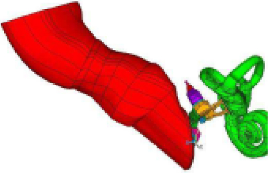
In this current work, the external auditory canal (EAC), middle ear, and inner ear (spiral cochlea, vestibule, and semi-circular canals) were modelled based on human temporal bone histological sections.
METHODS:
Multiple acoustic, structure, and fluid-coupled analyses were conducted using the FEM to perform harmonic analyses in the 0.1–10 kHz range. Once the FEM had been validated with published experimental data, its numerical results were used to calculate the EA or energy reflected (ER) by the tympanic membrane. This EA was also measured in clinical audiology tests which were used as a diagnostic parameter.
RESULTS:
A mathematical approach was developed to calculate the EA and ER, with numerical and experimental results showing adequate correlation up to 1 kHz. Another published FEM had adapted its boundary conditions to replicate experimental results. Here, we recalculated those numerical results by applying the natural boundary conditions of human hearing and found that the results almost totally agreed with our FEM.
CONCLUSION:
This boundary problem is frequent and problematic in experimental hearing test protocols: the more invasive they are, the more the results are affected. One of the main objectives of using FEMs is to explore how the experimental test conditions influence the results. Further work will still be required to uncover the relationship between middle ear structures and EA to clarify how to best use FEMs. Moreover, the FEM boundary conditions must be more representative in future work to ensure their adequate interpretation.
1.Introduction
The human auditory system (HAS) is an essential tool in performing numerous daily tasks. Therefore, it is important to be able to assess the proper functioning of the HAS in the most efficient way possible. The HAS is more complex than one might think at first glance, and there are still mechanisms whose exact functioning is unknown, or for which there are only hypotheses, such as the process of feedback from the inner and outer hair cells in the Basilar Membrane. In addition to this, there is the difficulty of accessing the HAS, which is embedded in the skull. Any intervention beyond the eardrum requires perforation or opening of the skull, with the corresponding consequences. These special circumstances have led medicine and engineering to develop non-invasive methods to determine the correct functioning of the HAS and, in case of malfunction, detect any associated pathology. The first and simplest test is audiometry, which involves subjecting the patient to the identification of beeps at different frequencies, increasing the intensity until surpassing the hearing threshold, at which point the patient informs the technician of the beep. Audiometry determines our hearing capacity in terms of frequency and decibels. Despite its simplicity, this test requires the patient’s cooperation and is not applicable to babies or individuals who are not conscious at the time. The measurement of impedance and/or Absorbed or Reflected Energy has been presented as an optimal solution.
Moller [1] first introduced the use of calibrated sound sources as a means for measuring impedances. The technique involves introducing a transmitter and receiver of waves into the auditory canal, so that the difference in energy between the emission and reception is evaluated. This difference can be related to the impedances of the different subsystems of the middle and inner ear, allowing for the inference of possible pathologies. This method, with some modifications or performances, is now extensively used. The following research [2, 3, 4, 5] establishes an identical foundation in terms of the pressure source and receiver in the auditory canal. The difference between them lies in the technique used to approximate the calculation of eardrum impedance. Some of the studies from this time [6, 7] begin to relate variations in impedance and, consequently, absorbed and reflected energies, to potential hearing loss.
In recent years, numerous studies have been conducted to improve the measurement of acoustic impedances [8, 9, 10, 11, 12], introducing Wideband Tympanometry (WBT) to replace the original Tympanometry. Nowadays, WBT is widely accepted and used for the calculation of impedances and reflected and absorbed energies. To do this, a passive test is performed that does not require any action from the patient. Some of these studies are more descriptive of the process and its proper setup [8, 9], while others focus more on the relationship between the results and potential pathologies and hearing loss [10, 11, 12]. Norton or Thevenin equivalent sources are used for measuring device calibration, with only a single pressure measurement then being needed to calculate the external auditory canal (EAC) entrance impedance [13]. Other research has used the transfer function method, which relies on measuring the influence of the termination impedance on duct pressure [14], thereby requiring robust coupling of the device and the EAC [4, 6]. Lanoye et al. [15] proposed a third method using impedance probes containing separated pressure and volume velocity sensors, although high levels of disturbance of the sound field at the measuring position are a problem when using this technique.
Most studies published to date have employed the two first methods where a sound (pressure) source and measuring device are usually placed inside the EAC. This is to avoid discontinuity between the device and the EAC to avoid exciting higher-order modes [16, 17, 18, 19]. The frequencies of the minimum and maximum input impedances are mainly affected by the EAC length and its cross-sectional area. This means that the sound source and measurement device directly affect the impedance calculations because they change the canal length. One possible solution to this problem could be the application of inverse procedures to derive the EAC shape from its input impedance [12]. Thus, knowing the calculated cross-sectional area of the EAC allows the required eardrum impedance transformation for the energy calculations to be estimated.
To obtain middle ear diagnostics, the input impedances of the EAC measurements are transformed to represent the position of the eardrum and thus, record reflected energy (RE) and the energy absorbed, abbreviated as EA [5, 7, 8, 13, 14, 15, 16, 17, 18]. However, these impedance and energy results are often inaccurate. Thus, the main objective of this current work was to clarify the origin of possible errors in these measurements and their transformation as well as the consequences of these errors in terms of the impedances and energy calculated from them. In this sense, the use of finite element models (FEMs) is now widely accepted as an adequate and complementary research tool. Thus, this paper was based on several numerical simulations conducted using a FEM previously described and validated in the academic literature. This original work was first conducted for the outer and middle ear [27, 28], was then applied to an inner ear FEM by employing a semiautomatic algorithm [29] and was finally coupled to the previous outer and middle ear FEMs [30]. Therefore, this FEM presents a complete fluid-structure interaction between the EAC, tympanic membrane (TM), and the oval window.
TM modelling was a crucial innovation with respect to previous models because the elements it used were better formulated and thereby eliminated problems associated with ‘shear locking’ elements used in thin membranes. Thus, together with adequate mesh convergence analysis, TM modelling provides sufficient guarantees of correct results. This means that, apart from geometric uncertainties caused by natural variability, most inaccuracy in this type of modelling comes from the difficulty of discerning the mechanical properties of some components such as the TM, tensors, and joints, among others. In this current article, we used assumed values for these components without attempting to discuss their accuracy. We simulated different combinations to discern the impact of each subsystem in the human auditory system (AS), building on a previous paper with a similar methodology [31] that determined how the AS influences pressure distribution in the EAC.
In this context, over the past century, Rong Gan has led a research group that has published several FEMs that have become an important source of inspiration for other researchers developing FEMs [32, 33, 34, 35, 36]. Gan’s work has focused on calculating EAC and eardrum impedances as well as the EA and ER from the TM [36]. Our work differs from that of Gan et al. in two clear ways. First, their main objective was to calculate the relationship between three middle ear disorders (otitis media, otosclerosis, and ossicular chain disarticulation), as simulated in their FEM, and any changes in the EA. Second, in contrast, our objective was to determine how the AS subsystems affect EA. We employed a range of FEMs, with the most basic one comprising an EAC and eardrum, to calculate the impedances and EAs. This methodology has already been applied successfully in previous work which gave us a better understanding of the mutual influence of each part of the AS on these factors.
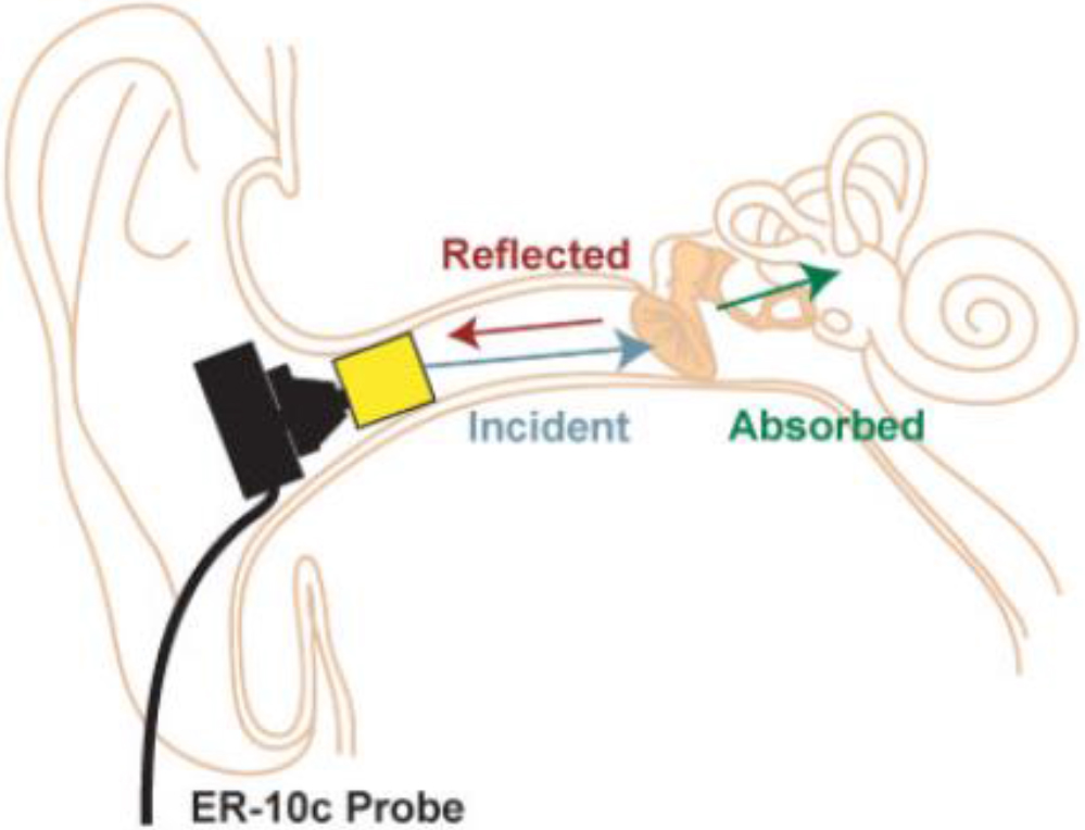
It is important to understand the differences in our strategic goals and those of Gan et al. because these differing objectives affect the simulation conditions employed. Gan and colleagues aimed to offer a useful tool for the diagnosis of middle ear disorders by testing EAs through pneumatic otoscopic and wideband absorbance audiometry tests. Therefore, they literally reproduced the experimental setup boundary conditions and placed the sound source 20 mm from the eardrum to simulate the experimental test conditions in the FEM (see Fig. 1). They determined that this approach gave them the best correlation between their numerical and experimental results. However, this does not mean that these numerical results most closely resemble reality. Indeed, controversy remains regarding the accuracy of the experimental methods used to measure impedance and in turn, the subsequent energy calculation results [37, 38, 39, 40, 41, 42]. Therefore, more theoretical background work will still be required to increase our knowledge in this area.
Figure 1.
A cross-section of the ear illustrating the probe used to measure impedance when inserted into the ear canal. The probe emits a sound pressure wave that is incident to the tympanic membrane. Some of the incident sound pressure is reflected and this is then measured by the probe. The remaining incident sound pressure is absorbed by the tympanic membrane and the structures behind it.
2.Method
2.1Theoretical background
The EA is calculated based on the ER. It describes the fraction of incident acoustic power reflected by the TM, where a reflective power of 1 corresponds to complete reflection of all acoustic power and a reflectance of 0 corresponds to the condition in which all power is absorbed by the TM [23]. First, the characteristic impedance of the EAC was calculated as:
(1)
where
(2)
The total TM impedance,
(3)
The acoustic impedance in the EAC was calculated based on
(4)
Where k is the wave number and L is the distance between the TM and the location of the measurement points in the EAC, which was at 30 mm in our study. The reflected acoustic pressure is obtained using the expression:
(5)
Thus, the ER is calculated based on the reflected acoustic pressure
(6)
Finally, the EA was obtained as a function of the frequency calculated as:
(7)
2.2Materials models
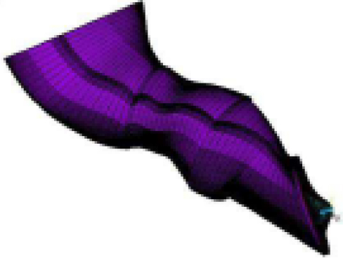
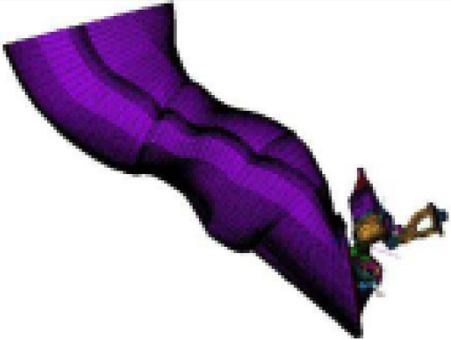
The construction and validation of the FEM applied in this section, as well as its material properties, have been previously published [27, 28, 29, 30]. However, in this current work, the EAC was re-meshed with hexahedral elements [43, 44] to help improve the accuracy of the FEM post-process calculations (Fig. 2).
Table 1
Combinations of different finite elements simulated in the CATI, CATIOS, and CATIOSCO finite element models
| Model | Subsystem modelled | Name |
|---|---|---|
| External auditory canal Tympanic membrane | CATI |
| External auditory canal Tympanic membrane Ossicular chain Cochlea simplified | CATIOS |
| External auditory canal Tympanic membrane Ossicular chain Cochlea Vestibuli Semicircular canals | CATIOSCO |
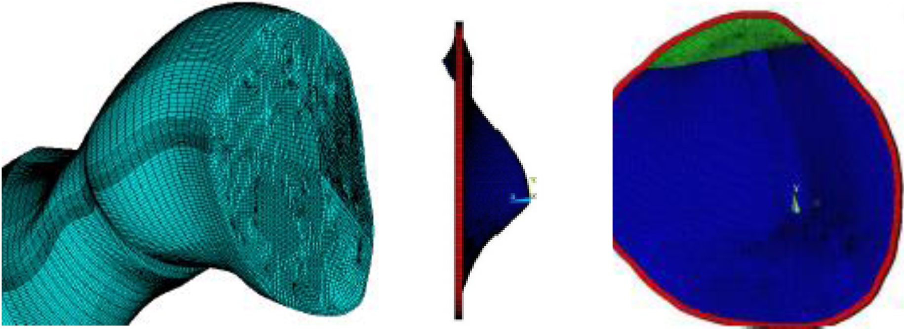
Figure 2.
Hexahedral finite element model (FEM) for the external auditory canal based on the tympanic membrane FEM.
As summarised in Table 1, three different FEM combinations were simulated to discern the impact of the different AS subsystems.
3.Computer simulation and results
The TM was modelled using 7,880 hexahedral elements, with each one itself comprising 8 nodes, although only the 4 that formed the surface in contact with EAC air were valid in our calculations. Thus, a total of 8,193 nodes formed the TM surface. With harmonic analysis, we obtained 16,386 real and imaginary values each for pressure and speed. Thus, when we performed the harmonic calculation for the 0.1–10 kHz range, we produced matrices comprising a total of 1,638,600 data points each for pressure and speed. In turn, the area was composed of only the 7,880 element data points. We then used ANSYS engineering simulation software to obtain a total of 3,285,080 values for use in impedance and EA calculations using MATLAB software.
3.1Tympanic membrane velocity
Figure 3.
The means for the tympanic membrane speed module for the three finite element models studied, CATIOSCO, CATI, and CATIOS. The CATI comprised the external auditory canal (EAC) and tympanic membrane (TM); CATIOS comprised the EAC, TM, ossicular chain (OC), and simplified cochlea; and CATIOSCO comprised the EAC, TM, OC, and the entire cochlea.
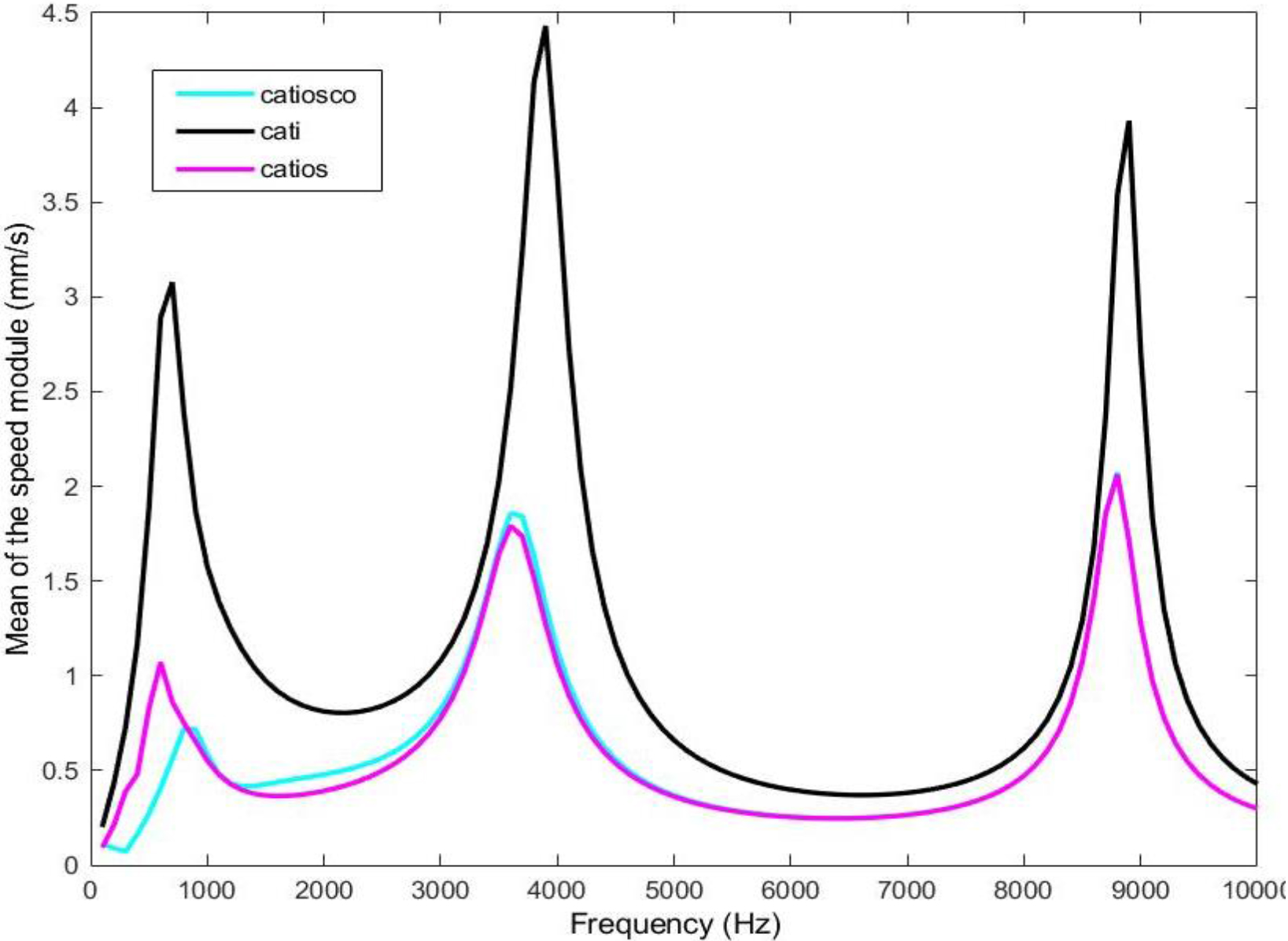
The average of all elements in the TM velocity module is shown in Fig. 3. There were three clearly differentiated resonance zones. One was at around 800–1,000 Hz because of the eardrum itself, while the other two, located at 4 kHz and 9 kHz, were the result of the characteristic resonances of the EAC [45]. These results highlight the importance of modelling the ossicular chain, as there is a significant difference in the outcomes when the ossicular chain and cochlea are not modelled. On the other hand, there are no significant differences observed between modelling the simplified cochlea and the realistic spiral model, resulting in significant computational savings.
3.2External auditory canal characteristic impedance
The characteristic impedance of the EAC, Zc depends on the air density (
Figure 4.
Comparison of the three studied finite element models with an experimental model by Zhang and Gan for the module (A) and phase (B) tympanic membrane impedance (ZTM).
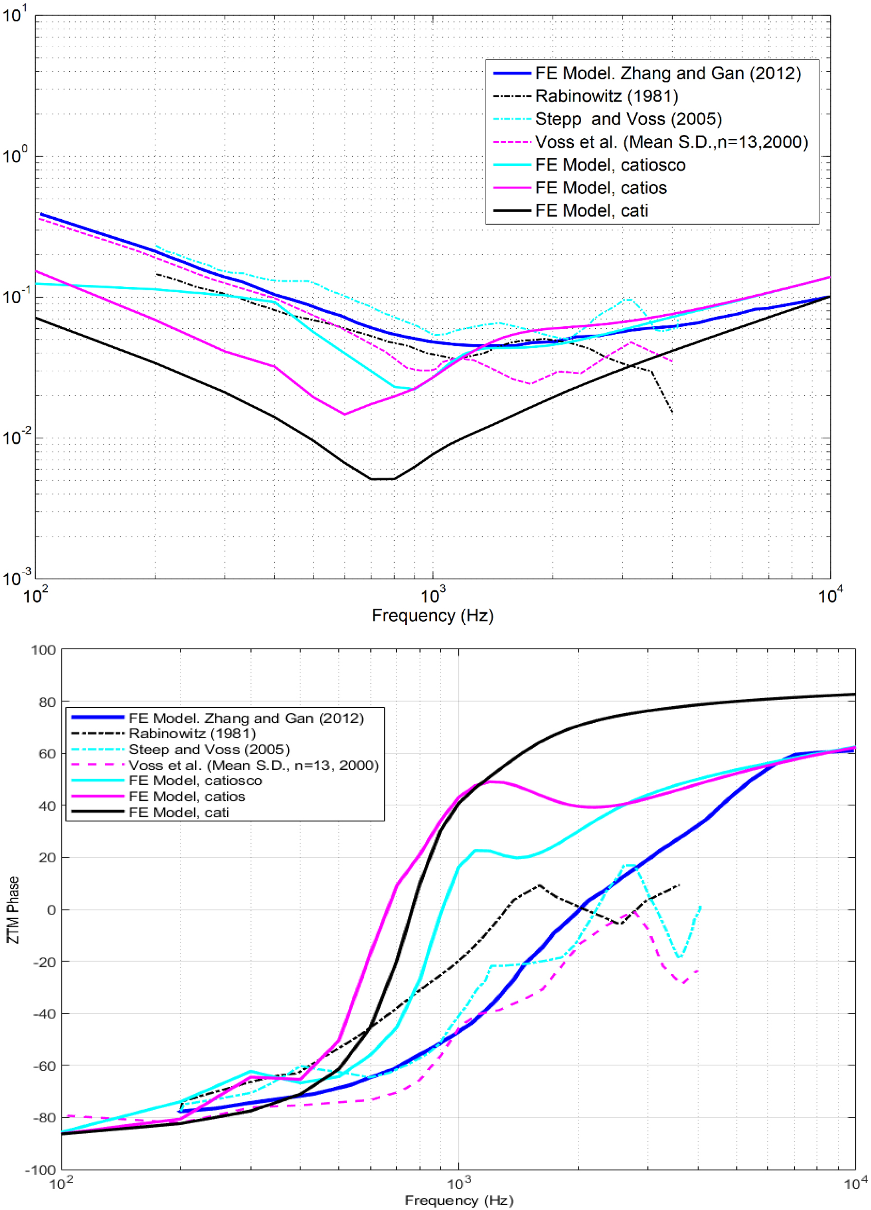
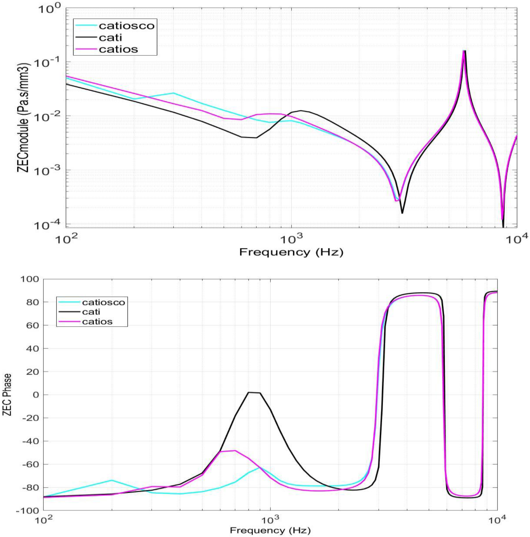
Figure 5.
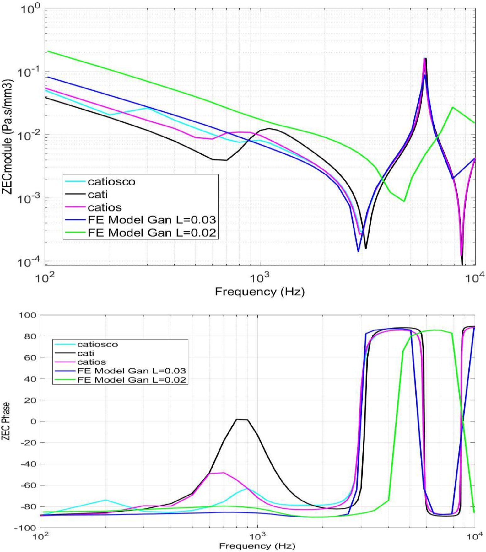
Comparison of the three studied finite element models for the module (A) and phase (B) external auditory canal impedance (ZEC).
3.3Tympanic membrane impedance (direct calculation)
Figure 4 represents the module and phase TM impedance in a frequency range of 0.1 to 10 kHz. Figure 4A shows a comparison of the module impedance for the three studied FEMs and showed a decrease in the impedance with frequency up to 800–1,000 Hz, after which it increased. This minimum coincided with the first eardrum resonance frequency in that range. Figure 4B shows how the system formed by the EAC and TM opposes the system of least resistance to wave propagation and so was where the highest speeds occurred. The phase impedance started at a value of
3.4External auditory canal impedance (backward calculation) based on tympanic membrane impedance
Figure 5A shows the module EAC impedance for each of the studied FEMs, which strongly coincided, especially at high frequencies. The EAC curves presented two minima, one at 3,000 Hz and the other at 9,000 Hz, with a maximum at around 6,000 Hz. In turn, Fig. 5B shows the phase EAC impedance curves for each FEM, which also strongly coincided at high frequencies. The WM stopped influencing the results in both the module and phase EAC impedance at around 1,000 Hz, with curve disturbances at a lower range than those present at 3,000, 6,000, or 9,000 Hz. The first and second resonance frequencies of the EAC were at 3,000 and 9,000 Hz, respectively, while the anti-resonance of the canal was at 6,000 Hz.
Figure 6.
Energy absorbed by the tympanic membrane for the different finite element models studied.
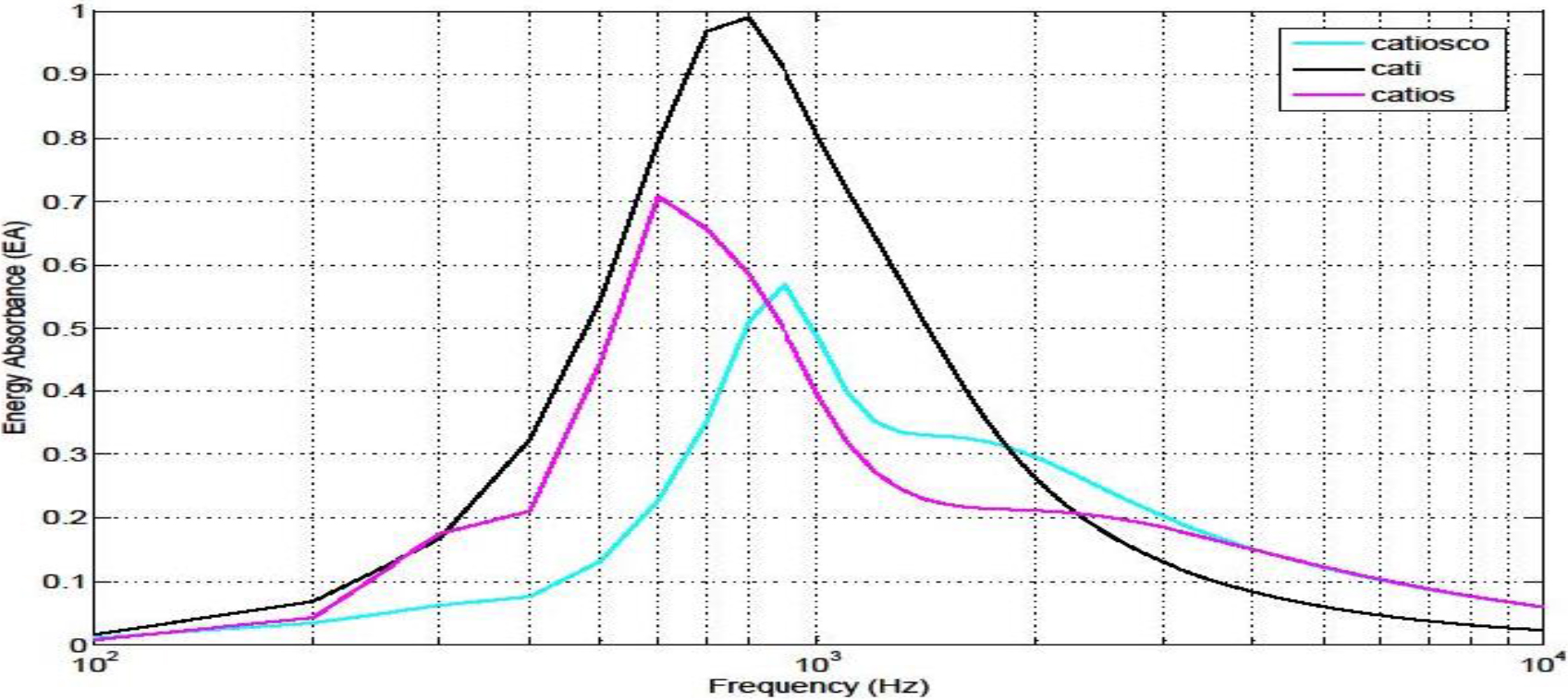
Figure 7.
Energy absorbed by the tympanic membrane for the finite element models and experimental results described in other publications.
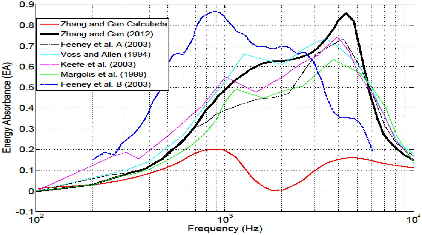
In Fig. 7 are shown the EA results published. Zhang [36] presented results from numerical simulations by FEM. Other results [5, 23, 25, 26] belongs to experimental tests. These experimental tests were carried out placing the pressure source inside the EAC, changing the natural EAC boundary conditions. There are differences between the experimental results, but It could be separate in two groups: on the one hand, Feeney et al. B, has the maximum before 1 kHz and fast decay; on the other hand, rest of experimental results have the maximum at 4 kHz. Our FEM results are more coincident with those presented by Feeney et al. B.
3.5Energy absorbance at the tympanic membrane
The results of EA for our models are presented In Fig. 6, the EA curve presented a maximum for a frequency value around 700–900 Hz in all three tested FEMs, reaching reaching a minimum for low frequency values between 100–200 Hz and a maximum at 9,000–10,000 Hz. Figure 6 shows how the maximum EA values coincided with the minimum of the MV impedance, as shown in Fig. 4B.
4.Conclusion
Figure 8.
Phase comparison of the module (A) and phase (B) external auditory canal impedance with the findings published by Zhang and Gan (2012).
To calculate the impedances, it appears that a well-defined cochlea model is unnecessary, especially at high frequencies. To validate this finding, we compared our data with those provided in previous academic publications. As shown in Fig. 8 for module (A) and phase (B) EAC impedance, the values obtained with our FEMs corresponded to the data obtained by Zhang and Gan [36]. The blue curve represents the impedance of the EAC calculated according to Zhang and Gan to which a correction method [42] was applied to simulate our test condition (L
Here we established a process for the numerical calculation of impedances and acoustic EA by the TM. This process starts with post-processing in ANSYS software followed by data exportation and processing in MATLAB. Regarding the impedance of the EAC, it is worth noting that the results obtained in this study agreed with those published by Gan and colleagues once the length of the canal was modified to 0.03 m, with values ranging from 10-4 to 10-1 Pa
In this study there are significantly differences when the ossicular chain and cochlea were introduced into the models. Without these elements, EA reached a value of almost 1 at around 900 Hz. This is quite logical because this frequency coincides with the first natural frequency of the eardrum at which almost all incoming energy is absorbed. When the ossicular chain and cochlea were modelled, this maximum value reduced to 0.6 and the frequency slightly increased to 1 kHz. Nonetheless, experimental results showed discrepancies in these figures. Previous work [46] exhibited a similar maximum EA frequency but with a value close to 1 while other results [5, 23, 25, 26, 36] showed that the first part was nearly identical to our findings in this current study, with a maximum around 1 kHz and a value of 0.6, except that the EA continued to increase to 3–4 kHz, with values between 0.7 and 1.
Considering the equation used to calculate EA (Eq. (7)) and referring to its root equations (Eqs (4)–(6)) involving ZTM, ZC, and ZEC (the TM and EAC impedances), we first showed that the ZTM we obtained coincided with the findings from experimental work presented elsewhere. Thus, we deduced that ZEC caused the differences between the modelled and experimental results mentioned above. This was because placement of the measuring device in the EAC considerably reduced its length, thereby affecting these impedance values, as demonstrated in Fig. 8. This may be because it is difficult to establish the conditions of a ‘normal ear’ as a FEM [23].
Conflict of interest
None to report.
Author contributions
A.G.-G. and C.C.-E. developed all FEMs in ANSYS software. J.A.-G. and P.C. carried out all post-processing in MATLAB software. P.L.-C. and A.G.-H. were the project coordinators and supervised all processes.
References
[1] | Møller AR. Improved Technique for Detailed Measurements of the Middle Ear Impedance. J Acoust Soc Am. (1960) ; 32. doi: 10.1121/1.1908029. |
[2] | Rabinowitz WM. Measurement of the acoustic input immittance of the human ear. J Acoust Soc Am. (1981) ; 70. doi: 10.1121/1.386953. |
[3] | Larson VD, Nelson JA, Cooper WA, Egolf DP. Measurements of acoustic impedance at the input to the occluded ear canal. J Rehabil Res Dev. (1993) ; 30. |
[4] | Keefe DH, Ling R, Bulen JC. Method to measure acoustic impedance and reflection coefficient. J Acoust Soc Am. (1992) ; 91. doi: 10.1121/1.402733. |
[5] | Voss SE, Allen JB. Measurement of acoustic impedance and reflectance in the human ear canal. J Acoust Soc Am. (1994) ; 95. doi: 10.1121/1.408329. |
[6] | Sanborn P-E. Predicting hearing aid response in real ears. J Acoust Soc Am. (1998) ; 103. doi: 10.1121/1.423082. |
[7] | Shahnaz N, Bork K, Polka L, Longridge N, Bell D, Westerberg BD. Energy Reflectance and Tympanometry in Normal and Otosclerotic Ears. Ear Hear. (2009) ; 30. doi: 10.1097/AUD.0b013e3181976a14. |
[8] | Jønsson S, Schuhmacher A, Ingerslev H. Wideband impedance measurement in the human ear canal; In vivo study on 32 subjects. Physics ArXiv: Medical Physics. (2018) . |
[9] | Niemczyk E, Lachowska M, Tataj E, Kurczak K, Niemczyk K. Wideband acoustic immitance – Absorbance measurements in ears after stapes surgery. Auris Nasus Larynx (2020) ; 47: : 909-23. doi: 10.1016/j.anl.2020.04.011. |
[10] | Chris S, Lisa H, Patrick F, Hideko H. Wideband Acoustic Immittance: Tympanometric Measures. Ear Hear. (2013) . |
[11] | Ellison JC, Gorga M, Cohn E, Fitzpatrick D, Sanford CA, Keefe DH. Wideband acoustic transfer functions predict middle-ear effusion. Laryngoscope. (2012) ; 122. doi: 10.1002/lary.23182. |
[12] | Keefe DH, Sanford CA, Ellison JC, Fitzpatrick DF, Gorga MP. Wideband aural acoustic absorbance predicts conductive hearing loss in children. Int J Audiol. (2012) ; 51. doi: 10.3109/14992027.2012.721936. |
[13] | Lawton BW, Shaw EAG. Estimation of acoustical energy reflectance at the eardrum from measurements of pressure distribution in the human ear canal. Journal of the Acoustical Society of America. (1982) ; 72: : 766-73. doi: 10.1121/1.388257. |
[14] | Utsuno H, Tanaka T, Fujikawa T, Seybert AF. Transfer function method for measuring characteristic impedance and propagation constant of porous materials. J Acoust Soc Am. (1989) ; 86. doi: 10.1121/1.398241. |
[15] | Lanoye R, Vermeir G, Lauriks W, Kruse R, Mellert V. Measuring the free field acoustic impedance and absorption coefficient of sound absorbing materials with a combined particle velocity-pressure sensor. J Acoust Soc Am. (2006) ; 119. doi: 10.1121/1.2188821. |
[16] | Hudde H, Letens U. Scattering matrix of a discontinuity with a nonrigid wall in a lossless circular duct. J Acoust Soc Am. (1985) ; 78. doi: 10.1121/1.392769. |
[17] | Fletcher NH, Smith J, Tarnopolsky AZ, Wolfe J. Acoustic impedance measurements-correction for probe geometry mismatch. J Acoust Soc Am. (2005) ; 117. doi: 10.1121/1.1879192. |
[18] | Stinson MR, Daigle GA. Transverse pressure distributions in a simple model ear canal occluded by a hearing aid test fixture. J Acoust Soc Am. (2007) ; 121. doi: 10.1121/1.2722214. |
[19] | Brass D, Locke A. The effect of the evanescent wave upon acoustic measurements in the human ear canal. J Acoust Soc Am. (1997) ; 101. doi: 10.1121/1.418244. |
[20] | Rasetshwane DM, Neely ST. Inverse solution of ear-canal area function from reflectance. J Acoust Soc Am. (2011) ; 130. doi: 10.1121/1.3654019. |
[21] | Shahnaz N, Bork K, Polka L, Longridge N, Bell D, Westerberg BD. Energy Reflectance and Tympanometry in Normal and Otosclerotic Ears. Ear Hear (2009) ; 30. doi: 10.1097/AUD.0b013e3181976a14. |
[22] | Allen JB, Jeng PS, Levitt H. Evaluation of human middle ear function via an acoustic power assessment. The Journal of Rehabilitation Research and Development. (2005) ; 42. doi: 10.1682/JRRD.2005.04.0064. |
[23] | Rosowski JJ, Nakajima HH, Hamade MA, Mahfoud L, Merchant GR, Halpin CF, et al. Ear-Canal Reflectance, Umbo Velocity, and Tympanometry in Normal-Hearing Adults. Ear Hear. (2012) ; 33. doi: 10.1097/AUD.0b013e31822ccb76. |
[24] | Sebothoma B, Khoza-Shangase K, Mol D, Masege D. The sensitivity and specificity of wideband absorbance measure in identifying pathologic middle ears in adults living with HIV. South African Journal of Communication Disorders. (2021) ; 68. doi: 10.4102/sajcd.v68i1.820. |
[25] | Piskorski P, Keefe DH, Simmons JL, Gorga MP. Prediction of conductive hearing loss based on acoustic ear-canal response using a multivariate clinical decision theory. J Acoust Soc Am. (1999) ; 105. doi: 10.1121/1.426713. |
[26] | Keefe DH, Simmons JL. Energy transmittance predicts conductive hearing loss in older children and adults. J Acoust Soc Am. (2003) ; 114. doi: 10.1121/1.1625931. |
[27] | Garcia-Gonzalez A, Castro-Egler C, Gonzalez-Herrera A. Analysis of the mechano-acoustic influence of the tympanic cavity in the auditory system. Biomed Eng Online. (2016) ; 15. doi: 10.1186/s12938-016-0149-2. |
[28] | Garcia-Gonzalez A, Gonzalez-Herrera A. Effect of the middle ear cavity on the response of the human auditory system. J Acoust Soc Am. (2013) ; 133. doi: 10.1121/1.4806416. |
[29] | Castro-Egler C, García-González A. Semiautomatic algorithm for 3D modelling of finite elements of the cochlea. J Med Imaging Health Inform. (2017) ; 7. doi: 10.1166/jmihi.2017.2136. |
[30] | García-González A, Durán-Escalante A, Castro-Egler C. 3D modelling and numerical analysis of human inner ear by means of finite elements method. International Journal of Computer and Information Engineering. (2016) ; 10: : 596--606. |
[31] | Garcia-Gonzalez A, Castro-Egler C, Gonzalez-Herrera A. Influence of the auditory system on pressure distribution in the ear canal. J Mech Med Biol. (2018) ; 18. doi: 10.1142/S0219519418500215. |
[32] | Gan RZ, Reeves BP, Wang X. Modeling of Sound Transmission from Ear Canal to Cochlea. Ann Biomed Eng. (2007) ; 35. doi: 10.1007/s10439-007-9366-y. |
[33] | Gan RZ, Sun Q, Feng B, Wood MW. Acoustic-structural coupled finite element analysis for sound transmission in human ear – Pressure distributions. Med Eng Phys (2006) ; 28. doi: 10.1016/j.medengphy.2005.07.018. |
[34] | Gan RZ, Feng B, Sun Q. Three-Dimensional Finite Element Modeling of Human Ear for Sound Transmission. Ann Biomed Eng. (2004) ; 32. doi: 10.1023/B:ABME.0000030260.22737.53. |
[35] | Brown MA, Bradshaw JJ, Gan RZ. Three-Dimensional Finite Element Modeling of Blast Wave Transmission From the External Ear to a Spiral Cochlea. J Biomech Eng. (2022) ; 144. doi: 10.1115/1.4051925. |
[36] | Zhang X, Gan RZ. Finite element modeling of energy absorbance in normal and disordered human ears. Hear Res. (2013) ; 301. doi: 10.1016/j.heares.2012.12.005. |
[37] | Nørgaard KR, Fernandez-Grande E, Laugesen S. Compensating for oblique ear-probe insertions in ear-canal reflectance measurements. J Acoust Soc Am. (2019) ; 145: : 3499-509. doi: 10.1121/1.5111340. |
[38] | Hudde H, Engel A. Measuring and modeling basic properties of the human middle ear and ear canal. Part III: Eardrum Impedances, Transfer Functions and Model Calculations. (1998) ; 84: . |
[39] | Hudde H, Engel A. Measuring and modeling basic properties of the human middle ear and ear canal. Part II: Ear Canal, Middle Ear Cavities, Eardrum, and Ossicles. (1998) ; 84: . |
[40] | Hudde H, Engel A. Measuring and modeling basic properties of the human middle ear and ear canal. Part I: Model Structure and Measuring Techniques. (1998) ; 84: . |
[41] | Hudde H. Measurement of the eardrum impedance of human ears. J Acoust Soc Am. (1983) ; 73. doi: 10.1121/1.388855. |
[42] | Fletcher NH, Smith J, Tarnopolsky AZ, Wolfe J. Acoustic impedance measurements-correction for probe geometry mismatch. J Acoust Soc Am. (2005) ; 117. doi: 10.1121/1.1879192. |
[43] | Ramos Valero JP. Modelado y análisis numérico con el método de los elementos finitos del canal auditivo externo y membrana timpánica. Málaga: s.n.; (2013) . |
[44] | Castro Egler C. Modelado 3D & Análisis Numérico del Oído Interno mediante Elementos Finitos. (2020) . |
[45] | Garcia-Gonzalez A, Castro-Egler C, Gonzalez-Herrera A. Influence of the auditory system on pressure distribution in the ear canal. J Mech Med Biol. (2018) ; 18. doi: 10.1142/S0219519418500215. |
[46] | Yilmaz N, Soylemez E, Sanuc MB, Bayrak MH, Sener V. Sound energy absorbance changes in the elderly with presbycusis with normal outer and middle ear. European Archives of Oto-Rhino-Laryngology (2023) ; 280: : 2265-71. doi: 10.1007/s00405-022-07742-8. |


