
An efficient 3D reconstruction method based on WT-TV denoising for low-dose CT images
Abstract
BACKGROUND:
In order to reduce the impact of CT radiation, low-dose CT is often used, but low-dose CT will bring more noise, affecting image quality and subsequent 3D reconstruction results.
OBJECTIVE:
The study presents a reconstruction method based on wavelet transform-total variation (WT-TV) for low-dose CT.
METHODS:
First, the low-dose CT images were denoised using WT and TV denoising methods. The WT method could preserve the features, and the TV method could preserve the edges and structures. Second, the two sets of denoised images were fused so that the features, edges, and structures could be preserved at the same time. Finally, FBP reconstruction was performed to obtain the final 3D reconstruction result.
RESULTS:
The results show that The WT-TV method can effectively denoise low-dose CT and improve the clarity and accuracy of 3D reconstruction models.
CONCLUSION:
Compared with other reconstruction methods, the proposed reconstruction method successfully addressed the issue of low-dose CT noising by further denoising the CT images before reconstruction. The denoising effect of low-dose CT images and the 3D reconstruction model were compared via experiments.
1.Introduction
In clinical diagnosis, doctors often use X-rays, ultrasound, and other equipment to obtain two-dimensional (2D) images of patients [1, 2]. Compared with the traditional diagnostic method, these techniques are extremely helpful in observing human tissue structures, extracting relevant information, and then determining reasonable treatment plans [3, 4]. However, it is difficult for doctors to obtain a clear three-dimensional (3D) spatial sense due to the blurred shape and size of human organs and tissues, relative spatial location, and adjacent relationship in 2D images [5, 6]. They can only infer the shape and size of the patient’s lesion and the relative location of the surrounding tissues and organs by observing multiple 2D tomographic images and their experience, and then make the corresponding diagnosis. Therefore, converting 2D tomographic images into a 3D reconstruction model is urgently required for contemporary clinical treatment [7, 8].
At present, many state-of-the-art 3D reconstruction methods have been proposed, which can be classified into three types: the analytics-based method, the iterative-based method, and the deep learning-based method. Xu et al. proposed the back-projection algorithm (BP) using the analytics-based method, which calculated the detection object value by projecting the reflection value [9]. Gordon et al. proposed the algebraic reconstruction technique (ART) using the iterative-based method, which transformed the reconstruction issue into a linear algebraic issue and reconstructed the image by iteratively optimizing the objective function [10]. Yao et al. proposed the MVSNet using the deep learning-based method, which was based on the binocular stereo matching of two images and extended the depth estimation to multiple images [11].
Although good results have been achieved using the aforementioned methods, many issues still persist, needing urgent attention. For example, the BP has deviation in the reconstructed images [12]. The performance of ART often requires a lot of data to optimize the iterative function [13]. When you use them like MVSNet, the deep learning-based methods require large amounts of data and are computationally intensive [14].
A pre-denoising 3D reconstruction method was proposed considering the advantages and disadvantages of the aforementioned methods and to address the issue of low-dose CT introducing more noise to reducing radiation [15]. It could remove most of the noise and retain the edges, structure, detailed features, and accuracy in the reconstruction model while reducing radiation, which helped the physician more accurately observe the overall morphology of the lesion and its relationship with the surrounding structures in multiple directions and angles [16].
The contributions of this study were as follows: (1) Edges, structures, detailed features, and accuracy of computed tomography (CT) images were preserved with reduced radiation. (2) The location and size of the tumor could be determined accurately in the 3D reconstruction model by extracting the information of 2D images.
The rest of this study is organized as follows. Section 2 briefly describes the related study. Section 3 presents the proposed model. Section 4 discusses extensive experiments used to evaluate the model. Section 5 concludes the study.
2.Related studies
2.1Computed tomography
CT is essentially an x-ray. Attenuation occurs when x-rays penetrate the human body [17]. X-rays passing through the human body carry different material densities of the attenuation signal received by the detector due to the different thicknesses of the human body, different densities of the tissues, and different compositions, are converted into visible light, and then are converted into an electrical signal by a photoelectric converter [18]. It is converted into a digital signal by an analog-to-digital converter, and finally a digital image of visible grayscale is reconstructed by a computer.
The radiation dose of CT is larger than that of ordinary x-ray machines. The low-dose CT was found to reduce the impact of radiation on the human body. Its radiation dose was only one-sixth to one-fifth of the ordinary CT [19]. However, reducing radiation results in another issue: more noise.
CT noise can be categorized into three types: (1) random noise, which may arise from the detection of a finite number of x-ray quanta in the projection. It is unpredictable and occurs randomly. (2) Quantum noise, which is also called statistical noise. It may be caused by the detection of a finite number of x-ray quanta in the projection. (3) Electronic noise, which is the noise generated by the CT hardware. Among these, quantum noise is the main noise [20].
2.2Wavelet transform
The wavelet transform (WT) is a mathematical tool for analyzing data whose features vary at different scales [21, 22]. For signals, the features can be time-varying frequencies, transients, or slowly changing trends. For images, the features include edges and textures. The WT was created primarily to address the limitations of the Fourier transform. The WT is a new method for wavelet analysis. It can analyze the local frequency in time (space) and gradually refine the signal (function) in multiple scales through the scaling and translation operation. Finally, it can achieve the time subdivision at high frequency and frequency subdivision at low frequency, which can automatically adapt to the requirements of time – frequency signal analysis.
Figure 1.
General process of WT.
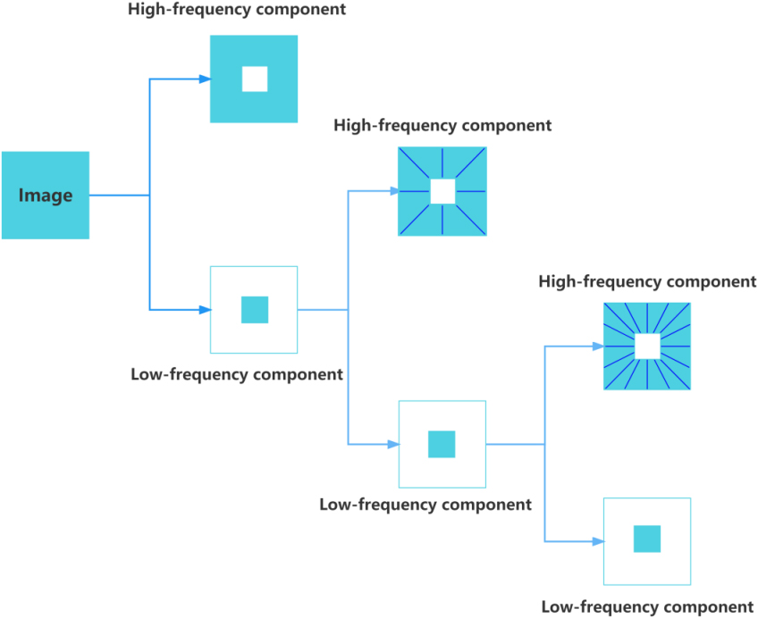
Figure 1 shows a three-level decomposition process of WT. An image can be divided into high-frequency and low-frequency parts, while the low-frequency part can be further decomposed into high-frequency and low-frequency parts, and so on, decomposed three times [23]. The WT is used to decompose the image into different frequency ranges using low-pass and high-pass filters so as to get each subband diagram. The energy of the image is concentrated to a few coefficients of some frequency bands through the WT because WT has the function of removing the correlation in the image and the energy concentration of the image [24]. The noise can be effectively suppressed by setting the wavelet coefficients in other bands to zero or giving them small weights, preserving important features.
2.3Total variation
The total variation (TV) is an anisotropic model that relies on the gradient descent method to smoothen the image [25]. It is expected to smoothen the image as much as possible because the difference between adjacent pixels is small, which does not smoothen the image.
The TV algorithm is an image restoration algorithm. It restores a clean image from a noisy image by building a noise model, solving the module using an optimization algorithm, and making the recovered image infinitely close to the ideal denoised image via a continuous iterative process [26]. The noise model is similar to the loss function in deep learning. The gap between the two gets closer through continuous training, and the gradient descent method is also required to quickly obtain the optimal solution. The advantage of the TV is that it allows sharp discontinuities, which is especially important for image denoising, such as edges or moving boundaries; these edges represent important features; the gradient descent method can be used to protect the edges well [27].
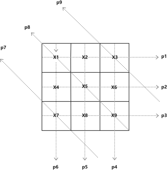
Figure 2.
Detection of a 2D slice.
2.4Filtered back-projection algorithm
Figure 2 shows a 2D slice of a 3D object. We divided it into discrete pixel regions and set the values in each pixel area to be uniformly distributed, representing the
(1)
We could find the value of each parameter to obtain the complete 2D slice image using Eq. (1), which is called the direct BP algorithm.
However, in the actual detection, each area is not uniformly distributed and noises are introduced during detection. Therefore, a filter was used to filter the projection, and an inverse Fourier transform was performed to obtain the filtered projection. Then this projection was back-projected to get our reconstruction result. The filtered back-projection (FBP) could correct the artifacts and the problems of edge blurring of direct back-projection, and the reconstruction result was clearer and more accurate [29, 30].
3.Proposed method
3.1Whole process
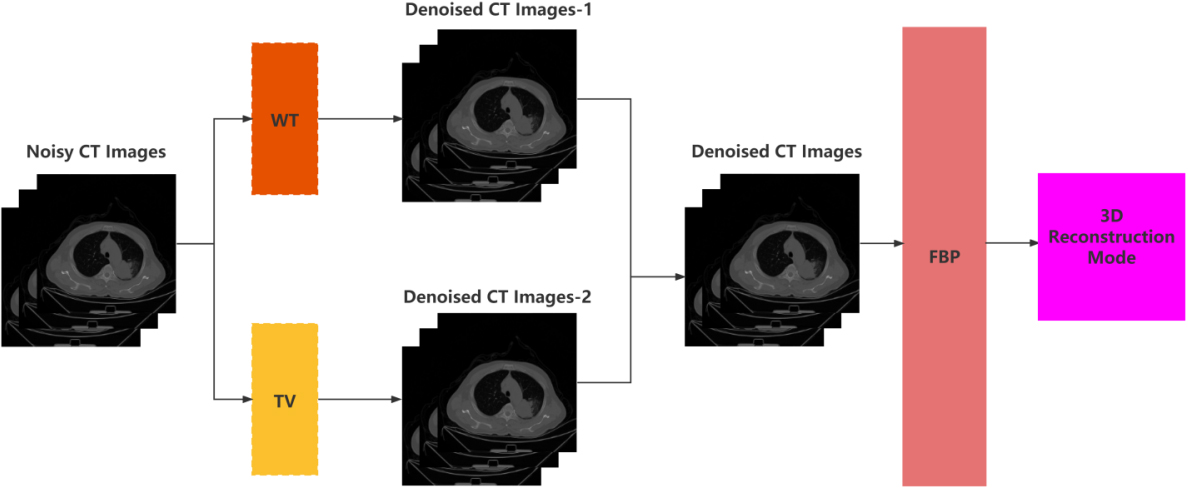
As shown in Fig. 3, the whole process consisted of the following steps. First, the WT and TV denoising were performed on the CT images. After the WT denoising, the features, edge, and structure could be well preserved after the TV denoising. Second, the two sets of images were fused to get the final denoised images. Finally, the fused images were reconstructed using the FBP.
Figure 3.
Whole process of the proposed method.
3.2WT denoising
A continuous periodic signal could be decomposed into a set of linear combinations of trigonometric signals with different frequencies, which was the essence of the Fourier series. The frequency of the signal could be obtained by taking a set of trigonometric functions as orthogonal bases and representing the original signal by a linear combination of this set of trigonometric bases. The process could be expressed as:
(2)
The infinite-length trigonometric basis was replaced by a finite-length decaying wavelet basis so that not only the frequency could be obtained but also the time could be located; this was called WT. It could be expressed as:
(3)
First, the image was used as the input and decomposed into high-frequency and low-frequency zones by a set of orthogonal wavelet bases. Then, the obtained low-frequency zone was used as the input signal and wavelet decomposition was performed again to obtain the next level of high-frequency and low-frequency zones, and so on. The high-frequency zone represented the detail coefficients. The low-frequency zone represented the approximation coefficients. After wavelet decomposition, the wavelet coefficients of the image were greater than the wavelet coefficients of the noise. Then, we threshold the wavelet decomposition coefficients, as depicted in Eq. (4), to separate the image from the noise.
(4)
3.3TV denoising
The TV of an image is depicted in Eq. (5). This represents the smoothness of an image. Generally, the smaller the TV value, the higher the smoothness. If an image has the same value for each pixel point, then this image has no fluctuations and its TV value is zero.
(5)
For an image containing noise, if the known signal has a certain level of smoothness, the TV algorithm can be used for denoising, which can be expressed as:
(6)
The TV constraint is a value that adjusts the degree of smoothness and the difference from the noise image. The larger the value, the smaller the difference between the final result and the noise image.
3.4Fusion
In the aforementioned process, we performed the WT and the TV denoising on CT images. The WT denoising algorithm could well preserve features, and the TV algorithm could well preserve edge and structural information. After the fusion of two sets of denoised images, the features, edges, and structures could be preserved at the same time, and a better denoising effect could be achieved.
We first decomposed images
(7)
3.5FBP reconstruction
In parallel beam projection, the projected value of a point is the sum of the projected values of all rays passing through the point in the plane, which can be expressed as:
(8)
Fourier transform was performed on the projection data as:
(9)
Then, the filter
(10)
Finally, the BP process could be expressed as:
(11)
4.Experiments and discussion
4.1Experiment setting
The experiments were performed in two parts: verifying the effectiveness of the denoising algorithm and the 3D reconstruction after denoising. We set the number of decomposition layers of WT to 3 (obtained by experimental effect comparison), the number of iterations of TV to 15, and the relaxation factor (Lagrange multiplier) to 0.03. We compared the algorithm with several state-of-the-art algorithms to verify the effectiveness of the proposed denoising algorithm: one filter-based algorithm BM3D [31], two model-based algorithms WNNM and TNRD [32, 33], and two learning-based algorithms DnCNN and FFDNet [34, 35]. We set the convolutional layer size of the DnCNN to 3
The computer system used for the experiments was CentOS Linux x64, CPU was Intel Xeon Silver 4114 CPU @ 2.20 GHz, and GPU was NVIDIA Tesla P100-PCIE 16 GB. The experimental code is implemented in Python 3.7, and the main frameworks include PyTorch 1.7.0 and OpenCV 4.4.0.
We used was the public data set LIDC-IDRI, and we selected 5000 images from this data set [38]. The main noise source of the low-dose CT was quantum noise, which obeyed the Poisson distribution. Hence, we added 10%, 15%, 20%, 25%, and 30% Poisson noise to the images [39].
Table 1
PSNR value of different denoising methods
| Methods | BM3D | WNNM | TNRD | DnCNN | FFDNet | WT-TV |
|---|---|---|---|---|---|---|
| Level | 30.04 | 29.83 | 30.05 | 30.12 | 30.26 | 30.38 |
| Level | 28.01 | 27.96 | 28.16 | 28.48 | 28.59 | 28.63 |
| Level | 26.35 | 26.22 | 26.38 | 26.42 | 26.65 | 26.44 |
| Level | 25.12 | 25.34 | 25.07 | 25.24 | 25.36 | 25.44 |
| Level | 23.63 | 23.60 | 23.31 | 23.71 | 23.88 | 23.90 |
4.2Results and discussion
Table 1 depicts the average PSNR values of different noise methods at five different noise levels of 10%, 15%, 20%, 25%, and 30%. It was seen that the WT-TV had the highest value. Compared with BM3D, WNNM, and TRND, their differences are more obvious when the noise is at levels 10 and 30, and very small at level 20, showing a U-shaped distribution. Compared with DnCNN and FFDNet, the PSNR values are only slightly higher than these two algorithms and do not vary with the noise level.
Table 2
SSIM value of different denoising methods
| Methods | BM3D | WNNM | TNRD | DnCNN | FFDNet | WTTV |
|---|---|---|---|---|---|---|
| Level | 0.872 | 0.875 | 0.875 | 0.882 | 0.875 | 0.853 |
| Level | 0.801 | 0.796 | 0.815 | 0.806 | 0.805 | 0.876 |
| Level | 0.762 | 0.763 | 0.774 | 0.781 | 0.786 | 0.790 |
| Level | 0.706 | 0.723 | 0.725 | 0.734 | 0.740 | 0.751 |
| Level | 0.663 | 0.703 | 0.701 | 0.714 | 0.718 | 0.723 |
Table 3
EPI value of different denoising methods
| Methods | BM3D | WNNM | TNRD | DnCNN | FFDNet | WTTV |
|---|---|---|---|---|---|---|
| Level | 0.97 | 0.95 | 0.95 | 0.96 | 0.97 | 0.98 |
| Level | 0.91 | 0.90 | 0.89 | 0.93 | 0.92 | 0.94 |
| Level | 0.85 | 0.56 | 0.83 | 0.87 | 0.87 | 0.89 |
| Level | 0.81 | 0.82 | 0.82 | 0.85 | 0.84 | 0.85 |
| Level | 0.72 | 0.73 | 0.72 | 0.76 | 0.78 | 0.78 |
Figure 4.
Denoising results of one image with noise level 10%.
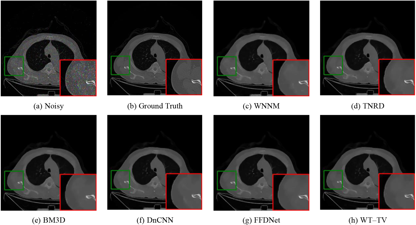
Table 2 depicts the average SSIM values of different noise methods at five different noise levels of 10%, 15%, 20%, 25%, and 30%. The WT-TV value was higher than that for the other methods. When the noise level is at 10, the SSIM value of WT-TV is lower than the other four methods, but when the noise level increases, its advantages will slowly manifest, especially when the noise level is at 15, it is significantly higher than the other four in amplification, and the difference is the largest.
Figure 5.
Denoising results of one image with noise level 15%.
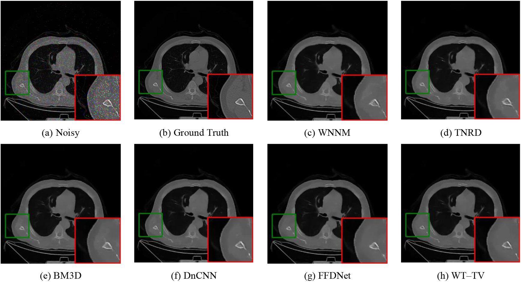
Figure 6.
Denoising results of one image with noise level 20%.
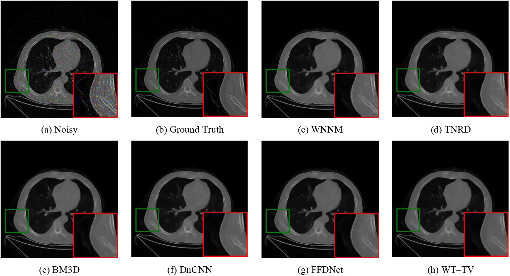
Figure 7.
Visual results of the 3D reconstruction model.
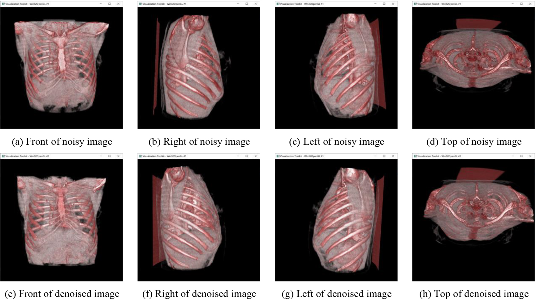
Figure 8.
Visual results of the 3D reconstruction model.
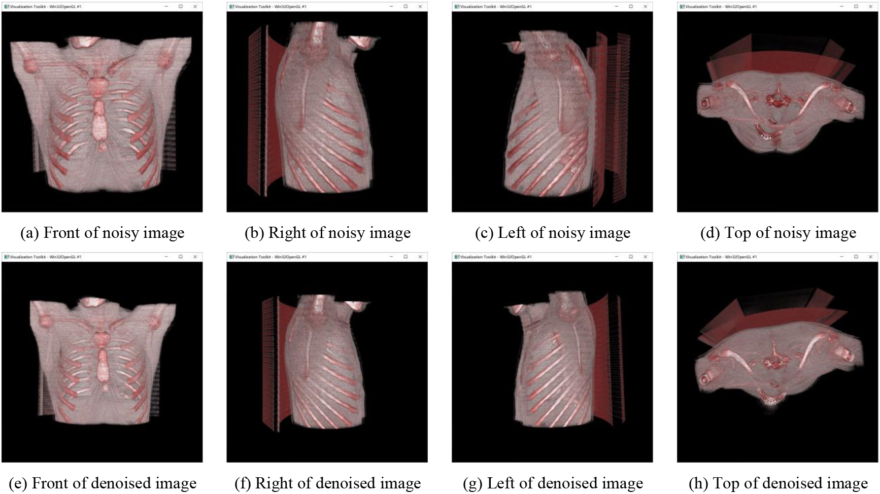
Table 3 depicts the average EPI values of different noise methods at five different noise levels of 10%, 15%, 20%, 25%, and 30%. The WT-TV achieved the best result among these methods. Overall, the EPI values of WT-TV are optimal at all levels of noise. Compared with BM3D, WNNM and TRND, with the maximum difference at level 20, and compared with DnCNN and FFDNet, there is an advantage but not very obvious.
Figures 4–6 show the visual results of the different methods. Only three groups are presented due to space limitations. The area marked by red squares is enlarged from the same position. Compared with the ground truth and noisy images, the ReBLS method retained more details than other methods and had the best denoising effect. In the enlarged area, we can compare the details of each method. The edge part of WT-TV denoising image is sharper and clearer, and the detail part is closer to the original picture.
Figure 9.
Visual results of the 3D reconstruction model.
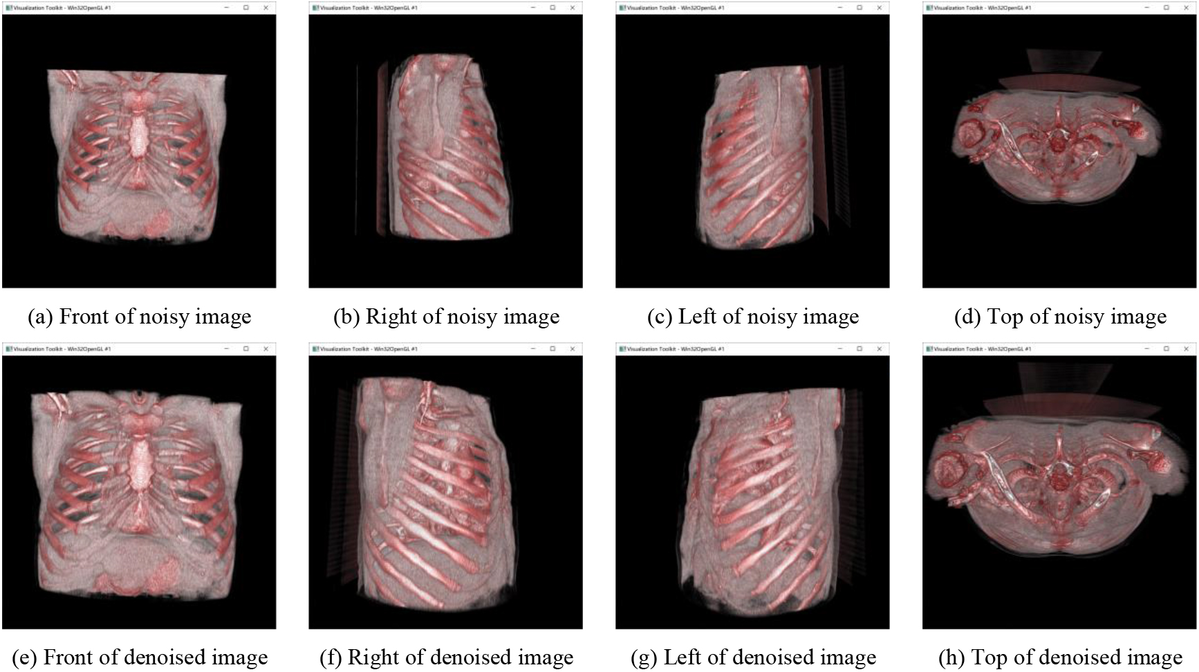
Figures 7–9 show the visual results of the 3D reconstruction models. Only three groups are presented due to space limitations. We took screenshots from the front, top, and left and right sides of the model to show the details. The images in (a)–(d) are 3D reconstructions of CT images without denoising, and the images in (e)–(h) are 3D reconstructions of CT images after denoising by WT-TV. We saw some artifacts around the 3D reconstruction model without denoising. Compared with the 3D reconstruction model without denoising, the distinction and structure of bones, organs, and muscles in the 3D reconstruction model after denoising were more clearly defined.
5.Conclusion
This study proposed an effective 3D reconstruction method for low-dose CT based on WT-TV denoising. Compared with other reconstruction methods, the reconstruction method used in this study successfully addressed the issue of low-dose CT noising by further denoising the CT images before reconstruction. The denoising effect of low-dose CT images and the 3D reconstruction model were compared via experiments. In all studies, the reconstructed models after denoising had clear structures, contours, and richer details.
The limitation of the proposed model was that it could be used only for CT images. Further studies are needed to focus on the generalizability of this model by applying it to other image data sets of different modalities.
Acknowledgments
The authors would like to thank the anonymous reviewers for their helpful comments and kind suggestions on this paper.
Conflict of interest
None to report.
Funding
This research received no external funding.
References
[1] | Zimmermann P, Peredkov S, Abdala PM, et al. Modern X-ray spectroscopy: XAS and XES in the laboratory. Coordination Chemistry Reviews. (2020) ; 423: : 213466. |
[2] | Allam AES, Khalil AF, Eltawab BA, et al. Ultrasound-guided intervention for treatment of trigeminal neuralgia: an updated review of anatomy and techniques. Pain Research and Management. (2018) ; 2018. |
[3] | Zhang YN, Fowler KJ, Hamilton G, et al. Liver fat imaging – a clinical overview of ultrasound, CT, and MR imaging. The British Journal of Radiology. (2018) ; 91: (1089): 20170959. |
[4] | Dinnes J, di Ruffano LF, Takwoingi Y, et al. Ultrasound, CT, MRI, or PET-CT for staging and re-staging of adults with cutaneous melanoma. Cochrane Database of Systematic Reviews. (2019) ; (7). |
[5] | Shirly S, Ramesh K. Review on 2D and 3D MRI image segmentation techniques. Current Medical Imaging. (2019) ; 15: (2): 150-160. |
[6] | Yu Q, Xia Y, Xie L, et al. Thickened 2D networks for efficient 3D medical image segmentation. arXiv preprint arXiv1904.01150, (2019) . |
[7] | Khan U, Yasin AU, Abid M, et al. A methodological review of 3D reconstruction techniques in tomographic imaging. Journal of Medical Systems. (2018) ; 42: (10): 1-12. |
[8] | Panayides AS, Amini A, Filipovic ND, et al. AI in medical imaging informatics: current challenges and future directions. IEEE Journal of Biomedical and Health Informatics. (2020) ; 24: (7): 1837-1857. |
[9] | Wang G, Qi F, Liu Z, et al. Comparison between back projection algorithm and range migration algorithm in terahertz imaging. IEEE Access. (2020) ; 8: : 18772-18777. |
[10] | Yang F, Zhang D, Huang K, et al. Incomplete projection reconstruction of computed tomography based on the modified discrete algebraic reconstruction technique. Measurement Science and Technology. (2018) ; 29: (2): 025405. |
[11] | Yao Y, Luo Z, Li S, et al. Mvsnet: Depth inference for unstructured multi-view stereo//Proceedings of the European conference on computer vision (ECCV). (2018) : 767-783. |
[12] | Willemink MJ, Noël PB. The evolution of image reconstruction for CT – from filtered back projection to artificial intelligence. European Radiology. (2019) ; 29: (5): 2185-2195. |
[13] | Bao P, Zhou J, Zhang Y. Few-view CT reconstruction with group-sparsity regularization. International Journal for Numerical Methods in Biomedical Engineering. (2018) ; 34: (9): e3101. |
[14] | Yu Z, Gao S. Fast-mvsnet: Sparse-to-dense multi-view stereo with learned propagation and gauss-newton refinement//Proceedings of the IEEE/CVF Conference on Computer Vision and Pattern Recognition. (2020) : 1949-1958. |
[15] | Pinsky PF. Lung cancer screening with low-dose CT: a world-wide view. Translational Lung Cancer Research. (2018) ; 7: (3): 234. |
[16] | Tong YH, Yu T, Zhou MJ, et al. Use of 3D printing to guide creation of fenestrations in physician-modified stent-grafts for treatment of thoracoabdominal aortic disease. Journal of Endovascular Therapy. (2020) ; 27: (3): 385-393. |
[17] | Withers PJ, Bouman C, Carmignato S, et al. X-ray computed tomography. Nature Reviews Methods Primers. (2021) ; 1: (1): 1-21. |
[18] | Hayashi K, Korecki P. X-ray fluorescence holography: principles, apparatus, and applications. Journal of the Physical Society of Japan. (2018) ; 87: (6): 061003. |
[19] | Moen TR, Chen B, Holmes DR, III., et al. Low-dose CT image and projection dataset. Medical Physics. (2021) ; 48: (2): 902-911. |
[20] | Diwakar M, Kumar M. A review on CT image noise and its denoising. Biomedical Signal Processing and Control. (2018) ; 42: : 73-88. |
[21] | Rhif M, Ben Abbes A, Farah IR, et al. Wavelet transform application for/in non-stationary time-series analysis: a review. Applied Sciences. (2019) ; 9: (7): 1345. |
[22] | Zhang D. Wavelet transform//Fundamentals of image data mining. Springer, Cham, (2019) : 35-44. |
[23] | Song Y, Zeng S, Ma J, et al. A fault diagnosis method for roller bearing based on empirical wavelet transform decomposition with adaptive empirical mode segmentation. Measurement. (2018) ; 117: : 266-276. |
[24] | Tan L, Chen Y, Zhang W. Multi-focus Image Fusion Method based on Wavelet Transform//Journal of Physics: Conference Series. IOP Publishing. (2019) ; 1284: (1): 012068. |
[25] | Zou J, Shen M, Zhang Y, et al. Total variation denoising with non-convex regularizers. IEEE Access. (2018) ; 7: : 4422-4431. |
[26] | Shamouilian M, Selesnick I. Total variation denoising for optical coherence tomography//2019 IEEE Signal Processing in Medicine and Biology Symposium (SPMB). IEEE. (2019) : 1-5. |
[27] | Guntuboyina A, Lieu D, Chatterjee S, et al. Adaptive risk bounds in univariate total variation denoising and trend filtering. The Annals of Statistics. (2020) ; 48: (1): 205-229. |
[28] | Gong K, Kim K, Cui J, et al. The evolution of image reconstruction in PET: From filtered back-projection to artificial intelligence. PET Clinics. (2021) ; 16: (4): 533-542. |
[29] | Schofield R, King L, Tayal U, et al. Image reconstruction: Part 1 – understanding filtered back projection, noise and image acquisition. Journal of Cardiovascular Computed Tomography. (2020) ; 14: (3): 219-225. |
[30] | Lee NK, Kim S, Hong SB, et al. Low-dose CT with the adaptive statistical iterative reconstruction V technique in abdominal organ injury: comparison with routine-dose CT with filtered back projection. American Journal of Roentgenology. (2019) ; 213: (3): 659-666. |
[31] | Hasan M, El-Sakka MR. Improved BM3D image denoising using SSIM-optimized Wiener filter. EURASIP Journal on Image and Video Processing. (2018) ; 2018: (1): 1-12. |
[32] | Yang H, Park Y, Yoon J, et al. An improved weighted nuclear norm minimization method for image denoising. IEEE Access. (2019) ; 7: : 97919-97927. |
[33] | Reehorst ET, Schniter P. Regularization by denoising: Clarifications and new interpretations. IEEE Transactions on Computational Imaging. (2018) ; 5: (1): 52-67. |
[34] | Zhang K, Zuo W, Chen Y, et al. Beyond a gaussian denoiser: Residual learning of deep cnn for image denoising. IEEE Transactions on Image Processing. (2017) ; 26: (7): 3142-3155. |
[35] | Zhang K, Zuo W, Zhang L. FFDNet: Toward a fast and flexible solution for CNN-based image denoising. IEEE Transactions on Image Processing. (2018) ; 27: (9): 4608-4622. |
[36] | Egiazarian K, Ponomarenko M, Lukin V, et al. Statistical evaluation of visual quality metrics for image denoising//2018 IEEE International Conference on Acoustics, Speech and Signal Processing (ICASSP). IEEE. (2018) : 6752-6756. |
[37] | Sun Y, Xin Z, Huang X, et al. Overview of SAR image denoising based on transform domain//3D Imaging Technologies – Multi-dimensional Signal Processing and Deep Learning. Springer, Singapore. (2021) : 39-47. |
[38] | Clark K, Vendt B, Smith K, et al. The Cancer Imaging Archive (TCIA): Maintaining and Operating a Public Information Repository. Journal of Digital Imaging. (2013) ; 26: (6): 1045-1057. doi: 10.1007/s10278-013-9622-7. |
[39] | Harper R, Flammia ST, Wallman JJ. Efficient learning of quantum noise. Nature Physics. (2020) ; 16: (12): 1184-1188. |


