
Comparative analysis of weka-based classification algorithms on medical diagnosis datasets
Abstract
BACKGROUND:
With the advent of 5G and the era of Big Data, the rapid development of medical information technology around the world, the massive application of electronic medical records and cases, and the digitization of medical equipment and instruments, a large amount of data has accumulated in the database system of hospitals, which includes clinical diagnosis data and hospital management data.
OBJECTIVE:
This study aimed to examine the classification effects of different machine learning algorithms on medical datasets so as to better explore the value of machine learning methods in aiding medical diagnosis.
METHODS:
The classification datasets of four different medical fields in the University of California Irvine machine learning database were used as the research object. Also, six categories of classification models based on the Bayesian theorem idea, integrated learning idea, and rule-based and tree-based idea were constructed using the Weka platform.
RESULTS:
The between-group experiments showed that the Random Forest algorithm achieved the best results on the Indian liver disease patient dataset (ILPD), delivery cardiotocography (CADG), and lymphatic tractography (LYMP) datasets, followed by Bagging and partition and regression tree. In the within-group algorithm comparison experiments, the Bagging algorithm achieved better results than other algorithms based on the integration idea for 11 metrics on all datasets, mainly focusing on 2 binary datasets. Logit Boost had only 7 metrics with significant performance, and the best algorithm was Rotation Forest, with 28 metrics achieving optimal values. Among the algorithms based on tree ideas, the logistic model tree algorithm achieved optimal results on all metrics on the mammographic dataset (MAGR). The classification performance of BFTree, J48, and Random Tree was poor on each dataset. The best algorithm was Random Forest on the ILPD, CADG, and LYMP datasets with 27 metrics reaching the optimum.
CONCLUSION:
Machine learning algorithms have good application value in disease prediction and can provide a reference basis for disease diagnosis.
1.Introduction
With the advent of 5G and the era of Big Data, the rapid development of medical information technology around the world, the massive application of electronic medical records and cases, and the digitization of medical equipment and instruments, a large amount of data has accumulated in the database system of hospitals, which includes clinical diagnosis data and hospital management data. The data sources are mainly electronic medical record systems, examination systems, testing systems, ultrasound systems, physical examination systems, and office automation systems. The analysis and mining of these data can gradually put together the information in the “fragmented” data accumulated in traditional medicine so as to present a more comprehensive picture of life conception and disease development. This can help people to have a more comprehensive and in-depth understanding of the mechanism of life and the principles of disease generation, thus improving the efficiency of disease prevention and control and clinical treatment.
With the continuous development of cross-cutting disciplines, a large number of machine learning and artificial intelligence algorithms are applied to medical datasets as an important component in disease prediction models, demonstrating excellent performance in medical-related fields such as disease prediction and assisted diagnosis, drug selection and application, and health insurance fraud and detection [1, 2, 3, 4]. As important artificial intelligence techniques such as data mining and machine learning, the decision tree algorithms in Weka are often used in basic medical research areas such as classification of DNA genes, classification and comparison of DNA barcodes, development and implementation of siRNA design tools, screening and differentiation of salt-loving and non-salt-loving proteins, and differentiation of classification properties of cell death-related proteins [5, 6, 7, 8, 9]. The main applications in the biomedical field are in the prediction, diagnosis, and treatment of diseases. J48 algorithm has achieved good results in diagnosing neonatal xanthogranuloma [10] and predicting the incidence of stroke using the k-nearest neighbor and C4.5 decision tree [11]. Also, scholars have used the multilayer perceptual decision tree algorithm to mine the decision of breast cancer treatment to assist doctors in the diagnosis and selection of hormone therapy, radiotherapy, chemotherapy, and other treatments [12], evaluation of the feasibility of support vector machine (SVM)-based diffusion tensor imaging for the classification of childhood sexual epilepsy disorders [13], and classification studies based on electroencephalogram (EEG) features of Alzheimer’s disease biomarkers [14], among others. In the area of hospital operations management services, the J48 algorithm has also been applied to machine learning related to electronic health record typing [15]. Stiglic [16] used supervised learning to select small datasets from medical error data that could be effectively predicted to enable the prediction of medical errors with a small set of datasets. SVMs were used to predict and design DrugMint, a web server for drug molecules [17]. Kaijian et al. [18] mined and analyzed chronic kidney disease data on the basis of the Weka data mining platform, and found that Random Forest (RF) performed better in the classification of chronic kidney disease datasets through algorithm comparison analysis. Ying et al. [19] used Weka software to build machine learning models. The results showed six algorithms with better classification prediction on the diabetes dataset: logistic model tree (LMT), sequential minimal optimization (SMO), Logistic, Naive Bayes, Rotation Forest, and Bagging. Yadin [20] employed the ID3 algorithm using data mining techniques to analyze dental consultation data. The ID3 algorithm was effectively improved, and the improved algorithm was again applied to the data. The accuracy greatly improved, and the researcher achieved the expected decision tree and classification rules.
Previous studies mostly applied single or several classifiers of the same type for modeling. The drawback of this approach was that algorithms that were truly applicable to a certain domain might be missed, and comprehensive modeling using algorithms based on different ideas was rarely used. In this study, we aimed to further explore the application of machine learning techniques in different medical fields by applying machine learning techniques to different medical prediction datasets using Weka data mining software, constructing multiple classification models, and analyzing the models through multiple performance evaluation metrics, so as to better inform hospital-oriented clinical and management applications.
2.Concepts and methods
Weka, a publicly available data mining workbench, assembles a large number of machine learning algorithms capable of undertaking data mining tasks, including pre-processing data, classification, regression, clustering, association rules, and visualization on a new interactive interface. In this study, we selected 24 machine learning algorithms in 6 major categories, which were highly representative (Table 1).
Table 1
Description of the classification algorithm
| Classification | Algorithm | Function description |
|---|---|---|
| Bayes | Naive Bayes | Standard probability plain Bayesian classifier |
| BayesNet | Learning Bayesian networks | |
| Bayesian Logistic Regression | Bayesian networks incorporating logistic regression | |
| Functions | SMO | A continuous minimum optimization algorithm for support vector |
| classification | ||
| Voted Perceptron | Voting perceptron algorithm | |
| RBF Network | Radial basis neural network | |
| Logistic | Building a linear logistic regression model | |
| Multilayer Perceptron | Neural networks with backward propagation (multilayer perceptron) | |
| Lazy | LWL | A general algorithm for locally weighted learning |
| KStar | Nearest neighbor algorithm using a generalized distance function | |
| IBk | K-nearest neighbor learner | |
| Meta | Bagging | Bagging algorithm: creating multiple models by sampling from raw data |
| Logit Boost | A forward stepwise addable model with a logarithmic loss function | |
| Dagging | Providing a subset of the classified training data to the chosen underlying | |
| learning algorithm | ||
| AdaBoostM1 | Adaptive boosting algorithm with an improved weight update function | |
| Rotation Forest | Rotating forest model | |
| Rules | Decision Table | Building a simple decision table majority classifier |
| PART | Obtaining rules from a partial decision tree built using J48 | |
| Tree | ADTree | Building an interactive decision tree |
| BFTree | Constructing a decision tree using a best-first search strategy | |
| J48 | C4.5 decision tree learner | |
| LMT | Combined tree structure and logistic regression models | |
| Random Forest | Constructing a Random Forest | |
| Random Tree | Constructing a tree where each node contains a specified number of | |
| random attributes |
The simple Bayesian algorithm is a commonly used probabilistic classification algorithm having the advantages of fast computation, high accuracy, and operational simplicity. In practical applications, it is assumed that the attributes in the samples affect them independently of each other. Therefore, it is productive for most of the more complex problems. Algorithms such as multilayer perceptron, logistic regression, and neural networks are function-based classification algorithms, and some of these algorithms are based on kernel functions and some on decision functions. Locally weighted learning (LWL) is an important algorithm in lazy learning. When a new instance needs to be processed, the distance between the training instance and the test instance is calculated using a distance function to determine a weighted set of training instances associated with the test instance, which is then used to construct a new model to process the new instance. The Euclidean distance is usually used to measure the distance between instances in traditional weighted learning algorithms. The Bagging algorithm, which was proposed by Breiman, was one of the first and the simplest integration method with the best performance. The basic principle is mainly to use a weak classification algorithm and an original training set. The learning algorithm is used to train classifiers in multiple rounds. Each round of training requires a bootstrap procedure to randomly have put-back sampling from the original training set to reconstitute a new training set for training a base classifier. After the training is completed, a sequence of prediction functions can be obtained, and eventually the individual prediction functions are classified using the simple voting method for the samples to be tested. Each random sampling obtains a different subset of training samples; hence, different base classifiers are trained, thus ensuring the diversity of the base classifier. The partition and regression tree (PART) decision tree algorithm, an algorithm invented in 1998 by Eibe Frank and Ian H. Witten, is an algorithm that uses incomplete decision trees to extract rules in a dataset. RF, J48, and other algorithms are based on decision trees. RF involves bootstrap aggregation in integration learning. The basic idea is to train a set of identical base classifiers (decision trees) and integrate the predictions based on all base classifiers using the integration methods such as hard voting, weighted voting, and so forth to obtain the final prediction results.
3.Experiment
3.1Datasets
Four datasets from different medical fields were selected for experimentation in this study to analyze and determine the prediction accuracy of different data mining algorithms. Dataset 1 was a mammographic (MAGR) mass dataset that could be used to predict the severity (benign or malignant) of the lumps. The mammographic lumps were analyzed based on Breast Imaging Reporting and Data System attributes and patient age. Dataset 2 was the Indian liver disease patient dataset (ILPD). This dataset was collected by 3 Indian professors from the northeastern part of Andhra Pradesh, India, and comprised 416 patients with liver cancer and 167 patients with non-hepatocellular cancer totaling 583 patients with the liver disease having 10 characteristics of medical data. Dataset 3 was a delivery cardiotocography (CADG) dataset to assess fetal status during pregnancy by recording fetal heart contraction tracing graphics, called cardiotocographs (CTGs). The accuracy of CTG diagnosis depends on the correct identification of fetal heart rate variability and uterine contraction characteristics. This dataset automatically processed 2126 fetal CTGs and measured the respective diagnostic characteristics. The CTGs were also classified in morphological form by three expert obstetricians, and a consensus classification label was assigned to each one. Dataset 4 was a lymphatic tractography (LYMP) dataset, and the output was classified into four categories: normal findings, metastases, malignant lymph, and fibrosis. At the same time, the original dataset was preprocessed separately in this study to make the prediction better (Table 2).
Table 2
Introduction to the datasets
| Serial number | Dataset | Types | Number of instances | Characteristic number | Number of output categories |
|---|---|---|---|---|---|
| 1 | MAGR | Binary classification | 961 | 6 | 2 |
| 2 | ILPD | Binary classification | 583 | 11 | 2 |
| 3 | CADG | Multiclassification | 2126 | 22 | 10 |
| 4 | LYMP | Multiclassification | 148 | 19 | 4 |
Table 3
Confusion matrix
| Actual category Class | Classifier category determination | |
|---|---|---|
| Determined to be Class | Judgment not Class | |
| Records belong to Class | True Positive (TP | False Negative (FN |
| Records are not part of Class | False Positive (FP | True Negative (TN |
3.2Evaluation indicators
This study aimed to better illustrate the prediction performance of the algorithms and compare the advantages and disadvantages of the algorithms intuitively. The evaluation metrics were determined according to the confusion matrix, mainly the kappa statistic, which was used to judge the degree of difference between the classification results of the classifier’s classification and the random classification, taking values in the range of [0, 1] for the supervised learning classification dataset. The results of the kappa statistical metrics were related to the area under the receiver operating characteristic curve (AUC) metrics of the classifier. Kappa
(1)
(2)
(3)
(4)
(5)
Moreover, a tenfold cross-validation approach was used for the training and prediction of the model. The scalability of the classification model was also an important metric used to measure the running time of a classification algorithm running on the same specific physical machine with the same disk and memory size that increased linearly with the change in the size of the database.
4.Analysis of experimental results
4.1Inter-group comparison analysis of classification algorithms
We selected one representative algorithm from each of the six major classes for interclass comparison analysis, including Naive Bayes, Logistic, LMT, Bagging, PART, and RF. As shown in Table 4, the
Table 4
Classification performance of the six algorithms on the four datasets
| Dataset | Algorithm | Kappa | MAE | RMSE | RAE | RRSE | TPR | 1-FPR | Precision | Recall | F-measure | Accuracy | AUC |
|---|---|---|---|---|---|---|---|---|---|---|---|---|---|
| MAGR | Naive Bayes | 0.5689 | 0.2397 | 0.4136 | 0.4819 | 0.8295 | 0.7850 | 0.7870 | 0.7870 | 0.7850 | 0.7850 | 0.7846 | 0.8510 |
| Logistic | 0.6445 | 0.2604 | 0.3586 | 0.5237 | 0.7191 | 0.8230 | 0.8220 | 0.8230 | 0.8230 | 0.8230 | 0.8231 | 0.8900 | |
| LWL | 0.6309 | 0.2666 | 0.3668 | 0.5362 | 0.7357 | 0.8190 | 0.8030 | 0.8280 | 0.8190 | 0.8160 | 0.8189 | 0.8910 | |
| Bagging | 0.6601 | 0.2416 | 0.3534 | 0.4859 | 0.7088 | 0.8310 | 0.8270 | 0.8310 | 0.8310 | 0.8310 | 0.8314 | 0.8960 | |
| PART | 0.6335 | 0.2357 | 0.3595 | 0.4739 | 0.7209 | 0.8180 | 0.8150 | 0.8180 | 0.8180 | 0.8760 | 0.8179 | 0.8760 | |
| Random Forest | 0.5811 | 0.2468 | 0.3935 | 0.4963 | 0.7892 | 0.7920 | 0.7890 | 0.7920 | 0.7920 | 0.7920 | 0.7919 | 0.8650 | |
| ILPD | Naive Bayes | 0.3791 | 0.3263 | 0.5635 | 0.6606 | 1.1338 | 0.6730 | 0.7300 | 0.7780 | 0.6730 | 0.6550 | 0.6733 | 0.7630 |
| Logistic | 0.4222 | 0.3672 | 0.4284 | 0.7433 | 0.8619 | 0.7080 | 0.7240 | 0.7240 | 0.7080 | 0.7080 | 0.7080 | 0.7780 | |
| LWL | 0.3597 | 0.3994 | 0.4500 | 0.8084 | 0.9055 | 0.6650 | 0.7170 | 0.7490 | 0.6650 | 0.6500 | 0.6647 | 0.7220 | |
| Bagging | 0.6199 | 0.2869 | 0.3619 | 0.5807 | 0.7281 | 0.8110 | 0.8140 | 0.8140 | 0.8110 | 0.8110 | 0.8107 | 0.8990 | |
| PART | 0.4764 | 0.3166 | 0.4243 | 0.6408 | 0.8536 | 0.7380 | 0.7440 | 0.7450 | 0.7380 | 0.7390 | 0.7380 | 0.8040 | |
| Random Forest | 0.7465 | 0.2426 | 0.3137 | 0.4911 | 0.6311 | 0.8740 | 0.8770 | 0.8760 | 0.8740 | 0.8740 | 0.8740 | 0.9510 | |
| CADG | Naive Bayes | 0.6615 | 0.0614 | 0.2186 | 0.3658 | 0.7547 | 0.7090 | 0.9630 | 0.7510 | 0.7090 | 0.7180 | 0.7093 | 0.9510 |
| Logistic | 0.7913 | 0.0448 | 0.1589 | 0.2471 | 0.5485 | 0.8250 | 0.9700 | 0.8240 | 0.8250 | 0.8240 | 0.8250 | 0.9790 | |
| LWL | 0.2990 | 0.1339 | 0.2556 | 0.7970 | 0.8823 | 0.4540 | 0.8490 | 0.3360 | 0.4540 | 0.3330 | 0.4544 | 0.9100 | |
| Bagging | 0.8206 | 0.0479 | 0.1491 | 0.2853 | 0.5148 | 0.8500 | 0.9680 | 0.8500 | 0.8500 | 0.8470 | 0.8504 | 0.9800 | |
| PART | 0.8024 | 0.0361 | 0.1754 | 0.2149 | 0.6054 | 0.8340 | 0.9680 | 0.8340 | 0.8340 | 0.8340 | 0.8344 | 0.9220 | |
| Random Forest | 0.8553 | 0.0479 | 0.1380 | 0.2854 | 0.4745 | 0.8790 | 0.9750 | 0.8780 | 0.8790 | 0.8770 | 0.8791 | 0.9880 | |
| LYMP | Naive Bayes | 0.9036 | 0.0399 | 0.1770 | 0.1075 | 0.4107 | 0.9280 | 0.9820 | 0.9340 | 0.9280 | 0.9290 | 0.9281 | 0.9820 |
| Logistic | 0.9090 | 0.0433 | 0.1667 | 0.1167 | 0.3868 | 0.9320 | 0.9800 | 0.9310 | 0.9320 | 0.9320 | 0.9325 | 0.9850 | |
| LWL | 0.7634 | 0.1017 | 0.2173 | 0.2737 | 0.5042 | 0.8280 | 0.9380 | 0.8960 | 0.8280 | 0.7700 | 0.8279 | 0.9840 | |
| Bagging | 0.9090 | 0.0548 | 0.1560 | 0.1475 | 0.3619 | 0.9320 | 0.9790 | 0.9330 | 0.9320 | 0.9320 | 0.9325 | 0.9900 | |
| PART | 0.9119 | 0.0348 | 0.1744 | 0.0936 | 0.4047 | 0.9350 | 0.9800 | 0.9340 | 0.9350 | 0.9340 | 0.9346 | 0.9720 | |
| Random Forest | 0.9442 | 0.0450 | 0.1318 | 0.1212 | 0.3059 | 0.9590 | 0.9880 | 0.9590 | 0.9590 | 0.9590 | 0.9586 | 0.9960 |
of multiple decision trees, each of which was different. In constructing the decision trees, a random portion of samples was selected from the training data with a put-back. Also, not all features of the data were used, but some features were randomly selected for training. Each tree used different samples and features, and the training results were different. The random process reduced the impact of influencing factors on the classification results. Although the results of the RF algorithm on the MAGR dataset were not satisfactory, the Bagging algorithm achieved better results, indicating that the RF algorithm was suitable for high-dimensional data with more features. From the perspective of dataset types, the group comparison algorithms selected in this study generally performed better on multiclass data than on dichotomous data.
4.2Intra-group comparison analysis of classification algorithms
This subsection conducted experimental validation for each of the three classes of algorithms to further verify the effectiveness and robustness of algorithms based on different ideas on different medical classification datasets. Among these, five metrics such as MAE, RMSE, RAE, RRSE, and FPR were negative metrics whose smaller values indicated better classification of the algorithms; the larger values of the remaining metrics indicated better classification of the algorithms.
4.2.1Meta-based algorithm
Ensemble learning is the combination of several weak classifiers (which can also be regressors) to produce a new classifier. As shown in Fig. 1, the Bagging algorithm outperformed the other algorithms on all datasets by 11 metrics, mainly on the 2 dichotomous datasets. Logit Boost, as a direct optimization of the binomial logarithmic loss Adaboost algorithm, had only seven metrics that performed significantly. Dagging provided a subset of the classified training data to the chosen base learning algorithm. The best algorithm was Rotation Forest, with a total of 28 indicators achieving optimal values, because the diversity of trees in the Rotation Forest was obtained by training each tree in the rotated feature space of the entire dataset before running the tree induction algorithm. Rotating the data axes created completely different classification trees. Besides ensuring tree diversity, the rotated trees reduced the constraints on the univariate trees that could decompose the input space to a hyperplane parallel to the original feature axes. More specifically, the complete feature set was created for each tree in the forest using a feature extraction approach. Principal component analysis (PCA) is a common unsupervised learning method that uses orthogonal transformations to transform observations represented by linearly correlated variables into data represented by several linearly uncorrelated variables. Each element was a linear combination of the original data. Further, the first major element was guaranteed to have the maximum variance. The other elements had high variance under the condition that they were orthogonal to the original elements, which showed that the RF algorithm was suitable for large data volume and high-dimensional linear classification data.
Figure 1.
Classification effect of the algorithm based on the integration idea.
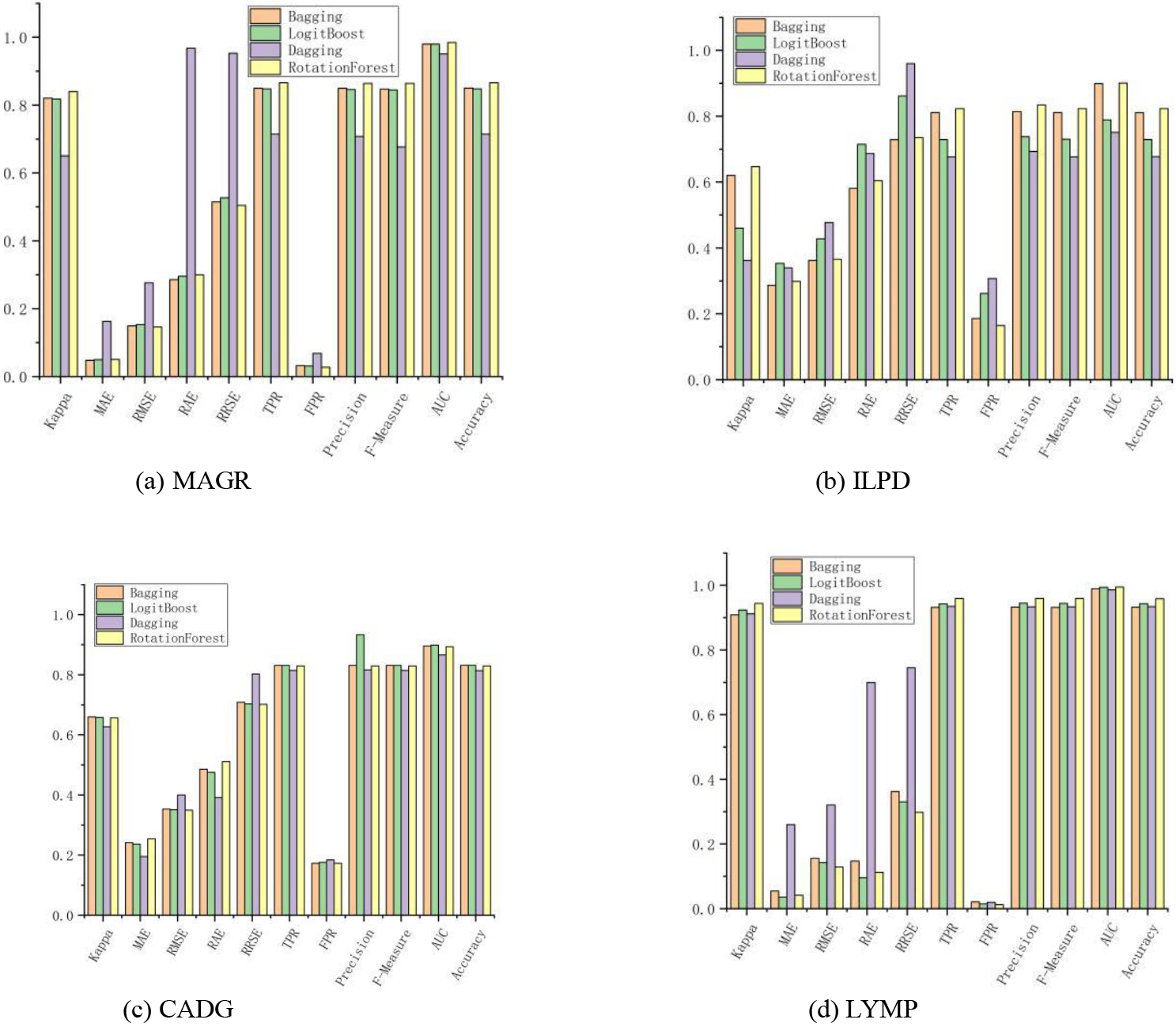
Figure 2.
Classification effect of the algorithm based on tree theory.
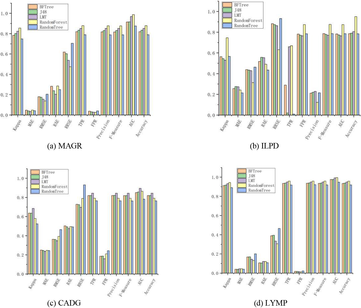
4.2.2Algorithm based on tree theory
For tree-thinking classifiers, the LMT algorithm achieved optimal results on all metrics on the MAGR dataset, which showed that the distance-based function classification was better under the small-sample low-dimensional linear condition as shown Fig. 2. BFTree, J48, and Random Tree performed poorly on each dataset. The best algorithm was RF, which achieved optimal results on the ILPD, CADG, and LYMP datasets with a total of 27 metrics reaching the optimum. In terms of the correct classification rate of the algorithms, all algorithms achieved more than 90% correct classification rate on LYMP, and the RF algorithm even exceeded 95%. The main idea of RF was to select a feature at each node of the tree from a subset of different attributes and replace the more general “random subspace approach” [21], which could be applied to many other algorithms such as SVMs. However, a recent comparison between RFs and random subspaces for decision trees has shown that the former is superior to the latter in terms of accuracy [22]. Other ways of adding randomness to the decision tree induction algorithm exist especially when numerical characteristics are involved. For example, instead of using all instances to decide the best splitting point for each numerical characteristic and using subsamples of instances [23] that are different. The optimal splitting criterion was evaluated using these characteristics and splitting points, which were chosen by each node decision. Since the sample selection for splitting at each node was different, the result of this technique was an ensemble of different tree combinations.
Table 5
Accuracy of various algorithms
| Class or classification | Algorithm | MAGR | ILPD | CADG | LYMP |
|---|---|---|---|---|---|
| Acc (%) | Acc (%) | Acc (%) | Acc (%) | ||
| Bayes | Naive Bayes | 78.46 | 67.33 | 70.93 | 92.81 |
| BayesNet | 82.83 | 70.87 | 73.71 | 95.86 | |
| Functions | SMO | 79.29 | 69.13 | 78.46 | 94.12 |
| RBF Network | 78.04 | 67.87 | 81.46 | 92.81 | |
| Logistic | 82.31 | 70.8 | 82.5 | 93.25 | |
| Multilayer Perceptron | 81.69 | 72.27 | 82.93 | 94.77 | |
| Lazy | LWL | 81.89 | 66.47 | 45.44 | 82.79 |
| KStar | 81.27 | 87.53 | 80.1 | 96.51 | |
| IBk | 75.55 | 75.47 | 78.65 | 95.42 | |
| Meta | Bagging | 83.14 | 81.07 | 85.04 | 93.25 |
| Logit Boost | 83.14 | 72.93 | 84.81 | 94.34 | |
| Dagging | 81.37 | 67.73 | 71.5 | 93.46 | |
| Rotation Forest | 82.93 | 82.27 | 86.59 | 95.86 | |
| Rules | Decision Table | 82.31 | 68.33 | 67.73 | 90.85 |
| PART | 81.79 | 73.8 | 83.44 | 93.46 | |
| Tree | BFTree | 82 | 78.2 | 81.98 | 93.46 |
| J48 | 82 | 77.2 | 83.4 | 93.9 | |
| LMT | 84.39 | 76.47 | 85.23 | 94.99 | |
| Random Forest | 79.19 | 87.4 | 87.91 | 95.86 | |
| Random Tree | 76.48 | 78.53 | 78.97 | 91.94 |
4.3Accuracy of the algorithm
Table 5 shows the results of the accuracy on the four datasets. The accuracy of KStar, Bagging, and Rotation Forest exceeded 80% on each dataset. The accuracy of all the algorithms except the LWL algorithm exceeded 91% on the LYMP dataset, with an average correct rate of 93.49%, of which KStar algorithm performed the best, reaching 96.51%. The performance of each algorithm on the MAGR dataset was more stable, with the correct rate concentrated at about 81.01%. The volatility of the performance of each algorithm was more obvious on the multiclass CADG dataset with multiple features, with accuracy rates ranging from 45.44% for LWL to 87.91% for RF, further illustrating the different generalizability of various algorithms, which should be noted in practical applications.
In this study, we compared and analyzed the algorithms of different ideas. The choice of of algorithm to be used in practical applications needs to be problem specific. It depends on many factors, such as the type and size of the data, the speed of training, the available computation time, the number of features, and the number of observations in the data. If the training data are small or the dataset has a small number of observation points and a large number of features such as genetic or textual data, an algorithm with high bias and low variance, such as linear regression, plain Bayes or linear SVM, should be chosen. If the training data are large enough and the number of observation points is larger than the number of features, a low-bias, high-variance algorithm, such as k-nearest neighbor, decision tree, or kernel SVM, can be used. A higher accuracy usually means longer training time, and the algorithms need more time to train the huge training data. Algorithms such as plain Bayes and linear and logistic regression are easy to implement and run quickly. SVM requires parameter tuning, neural networks need long convergence times, and RF algorithms need a lot of time to train the data. Further, better data often demands better algorithms, and well-designed features are equally important. Datasets may have a large number of features, and not all of these features may be relevant and important. For a certain type of data, such as genetic or textual data, the number of features may be extremely large compared with the number of data points. SVM is better suited for situations where the data have a large feature space and few observations. A large number of features may affect the performance of some learning algorithms, resulting in long training times. PCA and feature selection methods should be used to reduce the dimensionality and select important features.
5.Conclusions
In this study, we analyzed and evaluated the applicability and classification ability of each class of algorithms by comparing the effectiveness of machine learning algorithms on medical datasets with different patterns. Machine learning models can assist doctors to make predictions based on diagnosis and treatment information. However, in actual medical scenarios, doctors need to combine multiple aspects of patient information and their own empirical knowledge to comprehensively assess the disease. At the same time, they may encounter data category imbalance problems, multimodal data fusion problems, and knowledge reuse during classification and prediction. In the future, we can analyze and manage the patient consultation data by relying on our 360 panoramic electronic medical record system and Internet hospital platform. Also, we can develop more accurate prediction models, better integrate machine learning technology into the diagnosis and treatment analysis process, and truly play the role of assisting doctors through the introduction of classifier accuracy performance adjustment tools and the addition of more disease-specific test data.
Acknowledgments
The authors would like to thank Tianjin Baodi Hospital for providing the experimental platform.
Conflict of interest
None to report.
References
[1] | Jayanthi P. Machine learning and deep learning algorithms in disease prediction. Deep Learning for Medical Applications with Unique Data. (2022) ; 123-152. |
[2] | Kundu N, Rani G, Dhaka VS, et al. IoT and Interpretable Machine Learning Based Framework for Disease Prediction in Pearl Millet. Sensors. (2021) ; 21. |
[3] | Velswamy K, Velswamy R, Swamidason I, et al. Classification model for heart disease prediction with feature selection through modified bee algorithm. Soft Computing. (2021) ; 1-9. |
[4] | Mullaivanan D, Kalpana R. A Comprehensive Survey of Data Mining Techniques in Disease Prediction. (2021) . |
[5] | Mohammadmersad G, Taylor SJE, Pook MA, et al. Comparative (Computational) Analysis of the DNA Methylation Status of Trinucleotide Repeat Expansion Diseases. Journal of Nucleic Acids. (2013) ; 2013: : 689798. |
[6] | Weitschek E, Fiscon G, Felici G. Supervised DNA barcodes species classification: Analysis, comparisons and results. BioData Mining. (2014) ; 7: (1): 4. |
[7] | Chaudhary A, Srivastava S, Garg S. Development of a software tool and criteria evaluation for efficient design of small interfering RNA. Biochemical & Biophysical Research Communications. (2011) ; 404: (1): 313-320. |
[8] | Zhang G, Ge H. Support vector machine with a Pearson VII function kernel for discriminating halophilic and non-halophilic proteins. Computational Biology and Chemistry. (2013) ; 46: (10): 16-22. |
[9] | Carlos, Fernandez-Lozano, Marcos, et al. Markov mean properties for cell death-related protein classification. Journal of Theoretical Biology. (2014) ; 349: : 12-21. |
[10] | Ferreira D, Oliveira A, Freitas A. Applying data mining techniques to improve diagnosis in neonatal jaundice. BMC Medical Informatics and Decision Making. (2012) ; 12: (1): 143-143. |
[11] | Amini L, Azarpazhouh R, Farzadfar MT, et al. Prediction and control of stroke by data mining. International Journal of Preventive Medicine. (2013) ; 4: (Suppl 2): 5245. |
[12] | Abdülkadir C, Demirel B. A software tool for determination of breast cancer treatment methods using data mining approach. Journal of Medical Systems. (2011) ; 35: (6): 1503-1511. |
[13] | Amarreh I, Meyerand ME, Stafstrom C, et al. Individual classification of children with epilepsy using support vector machine with multiple indices of diffusion tensor imaging. NeuroImage: Clinical. (2014) ; 4. |
[14] | Kanda PAM, Trambaiolli LR, Lorena AC, et al. Clinician’s road map to wavelet EEG as an Alzheimer’s disease biomarker. Clinical Eeg and Neuroscience. (2014) ; 45: (2): 104-12. |
[15] | Peissig PL, Costa VS, Caldwell MD, et al. Relational machine learning for electronic health record-driven phenotyping. Journal of Biomedical Informatics. (2014) ; 52: : 260-270. |
[16] | Stiglic G, Kokol P. Discovering subgroups using descriptive models of adverse outcomes in medical care. Methods of Information in Medicine. (2012) ; 51: (4): 348-52. |
[17] | Dhanda SK, Singla D, Mondal AK, et al. DrugMint: A webserver for predicting and designing of drug-like molecules. Biology Direct. (2013) ; 8: (1): 28. |
[18] | Xia KJ, Wang JQ, Jin Y. Medical Data Classification and Early-prediction of Nephropathy Based on WEKA Platform. China Digital Medicine. (2018) . |
[19] | Zhang Y, Dou YF. Medical Data Classification and Early Diabetes Prediction Based on WEKA. Journal of Medical Information. (2021) ; 34: (6): 32-35. |
[20] | Roger J, Marshall, Richard J, et al. Quantifying the effect of age on short-term and long-term case fatality in 14,000 patients with incident cases of cardiovascular disease. European journal of cardiovascular prevention and rehabilitation: official journal of the European Society of Cardiology, Working Groups on Epidemiology & Prevention and Cardiac Rehabilitation and Exercise Physiology. (2008) . |
[21] | Ho TK. The random subspace method for constructing decision forests. IEEE Transactions on Pattern Analysis & Machine Intelligence. (1998) ; 20: (8): 832-844. |
[22] | Fernandez-Delgado M, Cernadas E, Barro S, et al. Do we need hundreds of classifiers to solve real world classification problems? Journal of Machine Learning Research. (2014) ; 15: : 3133-3181. |
[23] | Kamath C, Cantu-Paz E. Creating ensembles of decision trees through sampling: US, US 6938049 B2 [P]. (2005) . |


