
FNSAM: Image super-resolution using a feedback network with self-attention mechanism
Abstract
BACKGROUND:
High-resolution (HR) magnetic resonance imaging (MRI) provides rich pathological information which is of great significance in diagnosis and treatment of brain lesions. However, obtaining HR brain MRI images comes at the cost of extending scan time and using sophisticated expensive instruments.
OBJECTIVE:
This study aims to reconstruct HR MRI images from low-resolution (LR) images by developing a deep learning based super-resolution (SR) method.
METHODS:
We propose a feedback network with self-attention mechanism (FNSAM) for SR reconstruction of brain MRI images. Specifically, a feedback network is built to correct shallow features by using a recurrent neural network (RNN) and the self-attention mechanism (SAM) is integrated into the feedback network for extraction of important information as the feedback signal, which promotes image hierarchy.
RESULTS:
Experimental results show that the proposed FNSAM obtains more reasonable SR reconstruction of brain MRI images both in peak signal to noise ratio (PSNR) and structural similarity index measure (SSIM) than some state-of-the-arts.
CONCLUSION:
Our proposed method is suitable for SR reconstruction of MRI images.
1.Introduction
Magnetic resonance imaging (MRI) uses strong magnets, radio waves and computers to construct images, which is suitable for imaging soft tissues such as ligaments, tendons, and spinal cords. High-resolution images provide doctors with more abundant pathological information and improve the reliability of diagnosis. At present, obtaining higher resolution brain MRI image usually relies on two ways: extending scan time and using more sophisticated instruments [1]. However, extending scan time is not advisable because the patient is required to keep still for long time during scanning, while the use of more sophisticated instruments obviously causes imaging cost increase. The purpose of image super-resolution (SR) reconstruction [2] is to obtain a high-resolution (HR) image from low-resolution (LR) data through image processing techniques, which is more promising in improving brain MRI image quality.
SR reconstruction has a wide application in medical imaging [3], satellite imaging [4], security [5] and other fields. SR methods are divided into two main types: non-learning and learning. Non-learning methods are limited to requirement of prior knowledge. In contrast, learning-based methods obtains the prior knowledge directly from training samples [8, 9, 10] during learning process without assumption of the data distribution. In non-learning methods, linear interpolation methods such as bilinear and bi-cubic approaches [6, 7] are often used for SR. These methods are easy in implementation, however, they usually yield solutions with overly smooth textures. In learning methods, the sparse-coding-based method [9] is one of the important external example-based SR methods with assumption that the patches of HR and LR images have the same coefficients in sparse representation on their respective dictionaries, and an optimization problem is solved for generation of the final dictionaries. The solution is shared by most external example-based approaches, which are particularly focus on optimization of the dictionaries or establishment of efficient mapping formulations. However, this type of algorithm is based on certain prior conditions and the reconstruction result depends heavily on cumbersome parameter adjustment, resulting in a slow optimization for image reconstruction.
Since a shallow Convolutional Neural Network (CNN) was developed by Dong et al. [11], deep learning based algorithms have become more and more popular recently because of their superior ability in SR reconstruction. Based on SRCNN, the VDSR model was proposed by Kim [12] and obtain the reconstructed results in high quality. Dong et al. [13] proposed FSRCNN in which the low-resolution image with original size is directly used as input and the image is enlarged by the de-convolutional layer as the output, so as to speed up the network calculation. Lim et al. [14] constructed a very wide network EDSR by simplifying the residual blocks in residuals network (ResNet). Haris et al. proposed DBPN [15] through up and down projection to realize feature reuse. Zhang et al. [16] presented RDN in combination of residual and dense connections for improvement of the network performance. However, these networks such as EDSR and RDN require a large number of parameters. The recurrent structure can effectively make the network light-weighted. Specifically, DRCN [17] and DRRN [18] are regarded as a single-state RNN in which the information is shared in a feedforward manner with recurrent structure. For MRI image SR, many deep learning-based approaches have been developed. For instance, Schlemper et al. [19] used a deep cascade network to reconstruct dynamic MRI images. Shi et al. [20] built a wide residual network for SR reconstruction using fixed skip connections. However, these networks belong to feedforward frameworks, in which the shallow layers hardly access useful information from the deep layers. Recent studies [21, 22] have applied a feedback connection to the network, which transmit high-level signals to low-level layers and refine low-level information.
The feedback mechanism [21] is essentially implemented based on recurrent neural networks (RNNs). Although optimization operations such as partial connection and weight sharing can solve the long-distance dependence problem in recurrent neural networks, the information “memory” ability is still limited. In other words, the convolution in these optimization operations only extracts local features, without consideration of image global relationship, which makes the HR results short of hierarchy. Recently, the self-attention mechanism (SAM) is more reasonable in establishing global relationship in many fields [23, 24], allowing for measurement of the dependences between image positions with large distance.
To address the above issues, we propose a feedback network with SAM (FNSAM) for brain MRI imagine SR reconstruction. The feedback mechanism is implemented using RNN hidden states that at each iteration flows into the next iteration for modulation of the input features. The SAM is adopted to achieve the dependence among image pixels for reconstruction of the corresponding image using the global features. Our contributions are mainly described as follows:
1) The feedback mechanism is incorporated into the network such that the deep information is carried back to previous layers, which rescales the shallow feature information.
2) SAM is combined with the feedback network to generate more detailed information by capturing the global dependences from the high-level features of the image.
3) The proposed FNSAM achieves more correct texture details than many other SR methods.
2.Related work
2.1Feedback mechanism
For various vision tasks, the feedback mechanism has been explored by many network for carrying a notion of output to correct previous states, such as classification [21], human pose estimation [25], and other fields [26, 27]. These methods have a top-down feedback mechanism by using RNN structure. The SRFBN [22] is the first use of feedback mechanism in image SR, which concatenates the deep features of the previous iteration into the coarse feature extraction of current iteration. However, these methods directly transmit the high-level information to low-level layers, which lacks the ability to extract global features. SAM is focus on the key features for improvement of information representation. Therefore, in our method, the SAM is added to feedback network for extracting important features in feedback stage. Furthermore, the residual learning and dense skip connection are combined to build a rich image feature mapping of the network.
2.2SAM
The purpose of the attention mechanism is to focus on the details rather than the overall analysis. In recent years, spatial and channel attention mechanism has been applied to image super resolution reconstruction with promising results. Since the attention mechanism ensures that the input and output sizes remain the same, this design can be easily combined into a deep neural network for capturing dependencies in long-distance. For example, Zhang et al. proposed to use residual channel attention network to model channel correlation [28]. Dai et al. applied shifting channel attention to second-order attention enhancement [29]. Different from spatial and channel attention mechanisms, SAM exhibits promising in modeling global dependency. The SAM [30, 31] can establish the dependency relationship between the current concerned local location and all positions in the image, that is, the weighted dependency feature map of all local pixels in the image can be obtained while keeping the global features of the image. The brain MRI image exhibits non-local similarity which causes difficulty in capturing more efficient high-frequency information for super resolution reconstruction. This paper proposes to embed the SAM into the feedback network for paying attention to the weight between the pixels of the image itself, so as to enhance the expression ability of deep features in the feedback network.
3.Method
3.1FNSAM framework
Generation of a feedback network calls for several conditions. Firstly, for routing the feedback information into the input at next time step, the network should be recurrent over time. Secondly, to obtain the consistency between the output and input conditions, the feedback information flow is required to have the output image feature. Thirdly, the feedback information and low-level features are combined to be the total input. RNN is a necessary condition of feedback mechanism, in which the recurrent structure is used to achieve iterative process with a LR input provided at each time step for availability of low-level information and the loss is calculated to force the network to reconstruct a SR image that guides the LR image to restore a better SR result.
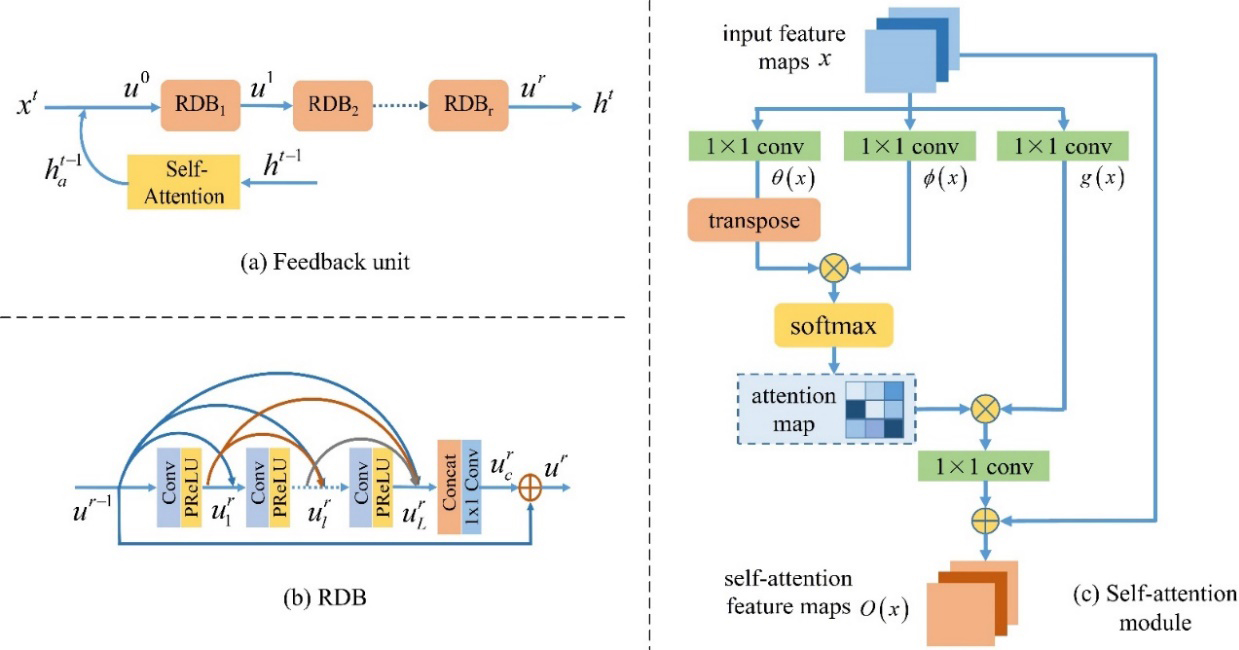
The proposed FNSAM is built by RNN with time steps of T, which is shown in Fig. 1. T sub-networks are contained in our unrolled FNSAM. Each sub-network can be regarded independent at a specific time step which consists of three parts with parameters shared across time steps: the input unit, feedback unit and the output unit.
Figure 1.
The structure of our FNSAM.

The input unit is the feature extraction stage, which includes two convolution layers for extraction of initial low-level features. The first and the second layers hold 3
Given
(1)
where
The feedback unit is the nonlinear feature mapping stage, which consists of multiple residual dense blocks (RDBs) and a self-attention module (SAM). Multiple RDBs are used to form a better features extraction hierarchy. The SAM receives high-level information from feedback connections and extract the attention maps for further refining the low-level features. In the feedback mechanism, the SAM is used to find the principle features
(2)
where
The output unit is the image reconstruction stage, including a de-convolutional layer and a convolutional layer. The deconvolutional layer is used to upscale the high-level features and the convolutional layer with 3
(3)
where
During each time step,
(4)
where
(5)
where
3.2Feedback unit
The structure of feedback unit is shown in Fig. 2. Stacking more RDBs will provide more various sizes of receptive field in each sub-network, which leads to a better hierarchy of extracted features. The HR image at the current time step is reconstructed using these features and the low-level features at the next time step are further modified. Because RDBs generate a large number of features and convolution is limited to local feature, the SAM is cooperated with feedback mechanism which can capture global dependencies and improve the accuracy of features.
Figure 2.
The proposed feedback unit with RDB and self-attention module.
The high-level features
(6)
where
The architecture of RDB is shown in Fig. 2b which is the same as the one in [16]. It contains dense connected layers, feature fusion and local residual learning. For each convolution layer, firstly, multiple trainable kernels are used to convolve the feature map of previous layer for extraction of the more informative features and generation of this layer feature maps. Then the activation function is used to non-linearize the convolutional result to yield more complex characteristics. The output
(7)
where
(8)
where
(9)
3.3Self-attention module
The self-attention module is divided into three branches, which decompose the input data into three components:
For the feature maps
(10)
where
Then, the attention map
(11)
where
It can be seen from the above description that the SAM model can focus on the pixel data of the whole area of the image. When integrated with deep features, the SAM can easily capture the main features in the whole spatial domain and enrich the context dependence according to the self-attention features.
4.Experimental and results
4.1Datasets and training settings
Medical images used in this paper are from the brain MRI dataset in The Cancer Imaging Archive (TCIA) [32] public database. We randomly select 80 representative images as the training dataset and 44 images as the test dataset which is divided into Test1 (8 images), Test2 (14 images) and Test3 (22 images). Data enhancement is performed on the selected training set using rotation and flips [33]. Specifically, the original images are rotated by 90
The first layer has 256 convolutional kernels and 64 RDBs. Because our purpose is to reconstruct MRI images, the number of input and output channels can be set to 1. Same as RDN [16], per RDB has 8 convolutional layers. The kernel size, stride, and padding of all convolutional layers in RDBs and the convolutional layer in output unit are set to 3, 1, and 1, respectively which can keep size fixed. A PReLU [35] activation function is used to follow all convolutional layers except the last convolutional layer of each RDB and the sub-network. The de-convolutional layer is set for each upscale factor as shown in Table 1.
Table 1
The settings for deconvolutional layer
| Scale factor | Kernel size | Stride | Padding |
|---|---|---|---|
| 6 | 2 | 2 | |
| 7 | 3 | 2 | |
| 8 | 4 | 2 |
The training image is divided into 48
4.2Ablation analysis
Table 2
The results of strategic ablation
| Methods | Combination of methods | ||
|---|---|---|---|
| Feedback network |
|
|
|
| SAM |
|
|
|
| PSNR | 32.64 | 33.13 | 33.16 |
| SSIM | 0.9027 | 0.9103 | 0.9104 |
To verify the effectiveness of feedback network and SAM, ablation analysis is performed. As shown in Table 2, the results of PSNR and SSIM on Test3 with upscale 4 reveal the advantage of feedback network and SAM. In the second group, it can be seen that using feedback network would perform better than the first group. This is mainly because RNN based feedback mechanism can reduce the errors occurring at each preceding time step. This further shows that the output feature map containing advanced information in the
4.3R and T analysis
The RDB number (denoted as R) and the time step number (denoted as T) are studied. Firstly, we construct various networks FNSAM-S (R
Table 3
The average results of different number of RDBs on TEST3 with scaling factor
| R | 4 | 5 | 6 | 7 |
|---|---|---|---|---|
| PSNR | 33.14 | 33.18 | 33.16 | 33.17 |
| SSIM | 0.9102 | 0.9105 | 0.9105 | 0.9105 |
Figure 3.
The convergence analysis of R.
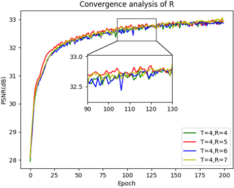
Figure 4.
The convergence analysis of T.
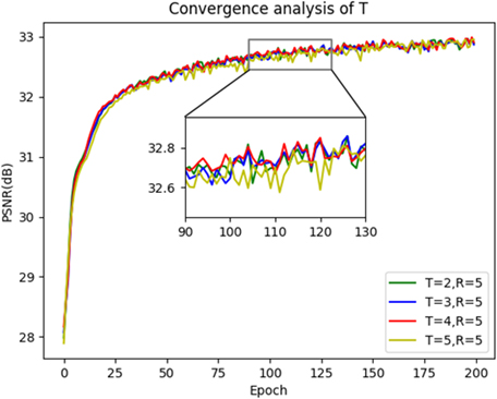
Table 4
The average results of different time step on TEST3 with scaling factor
| T | 2 | 3 | 4 | 5 |
|---|---|---|---|---|
| PSNR | 33.11 | 33.14 | 33.18 | 33.17 |
| SSIM | 0.9098 | 0.9101 | 0.9105 | 0.9104 |
Under identical setting of R
4.4Comparison with the state-of-the-arts
Table 5
Average PSNR for scale factor
| Dataset | Scale | Bicubic | ScSR | SRCNN | VDSR | EDSR | D-DBPN | RDN | SRFBN | FNSAM (ours) |
|---|---|---|---|---|---|---|---|---|---|---|
| Test1 | 37.11 | 38.06 | 40.20 | 40.67 | 40.75 | 40.68 | 41.37 | 41.51 | 41.57 | |
| 31.80 | 32.07 | 33.36 | 34.38 | 34.82 | – | 34.96 | 35.24 | 35.16 | ||
| 28.74 | 29.47 | 30.36 | 31.17 | 31.66 | 31.50 | 31.75 | 31.86 | 32.02 | ||
| Test2 | 38.06 | 39.56 | 40.90 | 42.06 | 42.47 | 42.20 | 42.34 | 43.44 | 43.47 | |
| 32.84 | 33.51 | 34.26 | 35.99 | 36.24 | – | 36.84 | 37.08 | 37.23 | ||
| 29.91 | 31.25 | 31.72 | 32.73 | 33.08 | 32.87 | 33.52 | 33.68 | 33.87 | ||
| Test3 | 37.69 | 39.01 | 40.65 | 41.79 | 41.85 | 41.82 | 42.59 | 42.73 | 42.78 | |
| 32.44 | 32.98 | 33.93 | 35.41 | 35.70 | – | 36.21 | 36.38 | 36.54 | ||
| 29.45 | 30.59 | 31.22 | 32.16 | 32.56 | 32.34 | 32.83 | 33.02 | 33.18 |
Table 6
Average SSIM for scale factor
| Dataset | Scale | Bicubic | ScSR | SRCNN | VDSR | EDSR | D-DBPN | RDN | SRFBN | FNSAM (ours) |
|---|---|---|---|---|---|---|---|---|---|---|
| Test1 | 0.9672 | 0.9755 | 0..9829 | 0.9838 | 0.9847 | 0.9840 | 0.9868 | 0.9876 | 0.9869 | |
| 0.8998 | 0.9174 | 0.9300 | 0.9372 | 0.9392 | – | 0.9413 | 0.9428 | 0.9439 | ||
| 0.8202 | 0.8460 | 0.8543 | 0.8732 | 0.8800 | 0.8758 | 0.8833 | 0.8856 | 0.8868 | ||
| Test2 | 0.9720 | 0.9796 | 0.9833 | 0.9859 | 0.9869 | 0.9863 | 0.9877 | 0.9886 | 0.9887 | |
| 0.9203 | 0.9356 | 0.9401 | 0.9497 | 0.9526 | – | 0.9554 | 0.9605 | 0.9600 | ||
| 0.8617 | 0.8745 | 0.8900 | 0.9115 | 0.9139 | 0.9117 | 0.9208 | 0.9236 | 0.9243 | ||
| Test3 | 0.9701 | 0.9782 | 0.9832 | 0.9851 | 0.9860 | 0.9858 | 0.9867 | 0.9879 | 0.9881 | |
| 0.9128 | 0.9290 | 0.9331 | 0.9469 | 0.9477 | – | 0.9521 | 0.9537 | 0.9545 | ||
| 0.8466 | 0.8605 | 0.8767 | 0.8976 | 0.9015 | 0.8985 | 0.9061 | 0.9093 | 0.9105 |
The proposed SR algorithm is compared with the current classical algorithms including ScSR [9], SRCNN [11], VDSR [12], EDSR [14], D-DBPN [15], RDN [16] and SRFBN [22] methods. Tables 5 and 6 show the average PSNR and SSIM for scale factor
Figure 5.
Visual results of different SR approaches for different scale factors.

Figure 5 gives the visualization of SR results using different methods. As shown in these figures, details are lost obvious in SR reconstruction produce by the bicubic interpolation. The proposed FNSAM alleviates the distortions and generates more accurate details in SR images compared with other methods. For example, the pattern in Fig. 5a is supposed to a vertical line. Affected by the surrounding stripe on the original image, other SR methods tend to reconstruct the curved pattern, and the proposed FNSAM can reconstruct the pattern correctly. In Fig. 5b and c, the proposed FNSAM can reconstruct the more obvious detail than others. In other words, our methods can recover clearer edges and more textures which are close to HR medical image than the comparison methods.
4.5Network performance and parameters
Figure 6.
Performance and number of parameters.
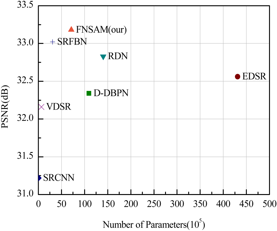
Figure 6 shows the comparison between the performance and parameters of some advanced SR methods and the proposed method on Test3 with upscale 4. As can be seen that parameters of SRCNN, VDSR and SRFBN methods are fewer but with lower PSNR than our proposed model. Our FNSAM achieves better performance and fewer parameters than D-DBPN, RDN and EDSR methods. This is attributed to the ability of RNN structure to decrease the parameters of the network.
5.Conclusion
In this paper, we have proposed a network called feedback network with self-attention mechanism (FNSAM) for SR reconstruction of brain MRI images. The feedback network is constructed according to the principle of recurrent neural network. By using the feedback function of the feedback network, the high-level information output from the network is returned to the low-level layers to optimize the shallow information. Moreover, the self-attention module is added in the feedback network to extract the principle features which promotes the visual hierarchy impress. The proposed FNSAM is capable of obtaining more natural HR brain MRI images. Quantitative and qualitative evaluation shows its advantages over those compared approaches. In further, we will be focus on study of SR networks for arbitrary magnification based on meta-learning.
Acknowledgments
This research was supported by the National Natural Science Foundation of China (No. 61501241), the Project of Jiangsu Transportation Department (No. 2021Y), and the Foundation of Shandong provincial Key Laboratory of Digital Medicine and Computer assisted Surgery (No. SDKL-DMCAS2018-04).
Conflict of interest
None to report.
References
[1] | Lusting M, Donoho D. Compressed sensing MRI. IEEE Signal Process. Mag. (2008) ; 25: : 72-82. |
[2] | Nan F, Zeng Q, Xing Y, et al. Single image super-resolution reconstruction based on the resnext network. Multimed Tools Appl. (2020) ; 79: : 34459-34470. |
[3] | Huang J, Wang L, Qin J, et al. Super-resolution of intravoxel incoherent motion imaging based on multisimilarity. IEEE Sens. J. (2020) ; 20: : 10963-10973. |
[4] | Cen X, Song X, Li Y, et al. A deep learning-based super-sesolution model for bistatic SAR image. Int. Conf. On ECIE, (2021) . |
[5] | Wang W, Hu Y, Li Y, et al. Brief survey of single image super-resolution reconstruction based on deep learning approaches. Sens Imaging. (2020) ; 21: : 21. |
[6] | Kacmaz RN, Yilmaz B, Aydin Z. Effect of interpolation on specular reflections in texture-based automatic colonic polyp detection. Int. J. Imag. Syst. Tech. (2021) ; 31: (1): 327-335. |
[7] | Hu J, Tang Y, Fan S. Hyperspectral image super-resolution based on multiscale feature fusion and aggregation network with 3-D convolution. IEEE J-STARS. (2020) ; 13: : 5180-5193. |
[8] | Yang J, Wang Z, Lin Z, et al. Coupled dictionary training for image super-resolution. IEEE Trans. Image Process. (2012) ; 21: : 3467-3478. |
[9] | Li X, Cao G, Zhang Y, et al. Combining synthesis sparse with analysis sparse for single image super-resolution. Signal Process-Image. (2020) ; 83: : 115805. |
[10] | Kim KI, Kwon Y. Single image super-resolution using sparse regression and natural image prior. IEEE Trans. Pattern Anal. (2010) ; 32: : 1127-1133. |
[11] | Dong C, Loy C, He K, et al. Learning A deep convolutional network for image super-resolution. Proc. Eur. Conf. Comput. Vis. (2014) ; 8692: : 184-199. |
[12] | Kim J, Lee K, Lee KM. Accurate image super-resolution using very deep convolutional networks. Proc. IEEE Conf. Comput. Vis. Pattern Recognit. (2016) ; 1: : 1646-1654. |
[13] | Dong C, Loy CC, Tang X. Accelerating the super-resolution convolutional neural network. Proc. Eur. Conf. Comput. Vis. (2016) ; 9906: : 391-401. |
[14] | Lim B, Son S, Kim H, et al. Enhanced deep residual networks for single image super-resolution. Proc. IEEE Conf. Comput. Vis. Pattern Recognit. (2017) ; 1: : 1132-1140. |
[15] | Haris M, Shakhnarovich G, Ukita N. Deep back-projection networks for super-resolution. In Proc. IEEE Conf. Comput. Vis. Pattern Recognit. (2018) ; 1664-1673. |
[16] | Zhang Y, Tian Y, Kong Y, et al. Residual dense network for image super-resolution. In Proc. IEEE Conf. Comput. Vis. Pattern Recognit. (2018) ; 1: : 2472-2481. |
[17] | Kim J, Lee JK, Lee KM. Deeply recursive convolutional network for image super-resolution. In Proc. IEEE Conf. Comput. Vis. Pattern Recognit. (2016) ; 1: : 1637-1645. |
[18] | Tai Y, Yang J, Liu X. Image super-resolution via deep recursive residual network. In Proc. IEEE Conf. Comput. Vis. Pattern Recognit. (2017) ; 1: : 2790-2798. |
[19] | Schlemper J, Caballero J, Hajnal JV, et al. A deep cascade of convolutional neural networks for dynamic MR image reconstruction. IEEE Trans. Medical Imaging. (2018) ; 37: : 491-503. |
[20] | Shi J, Li Z, Ying HS, et al. MR image super-resolution via wide residual networks with fixed skip connection. IEEE J. Biomed. Health Inform. (2019) ; 23: : 1129-1140. |
[21] | Zamir AR, Wu T, Sun L, et al. Feedback networks. In Proc. IEEE Conf. Comput. Vis. Pattern Recognit. (2017) ; 1: : 1808-1817. |
[22] | Li Z, Yang J, Liu Z, et al. Feedback network for image super-resolution. In Proc. IEEE Conf. Comput. Vis. Pattern Recognit. (2019) ; 3862-3871. |
[23] | Naseer MM, Ranasinghe K, Khan SH, et al. Intriguing properties of vision transformers. NIPS. (2021) ; 34: : 23296-23308. |
[24] | Li QM, Jia RS, Zhao CY, et al. Face super-resolution reconstruction based on self-attention residual network. IEEE Access. (2020) ; 8: : 4110-4121. |
[25] | Kocabas M, Athanasiou N, Black MJ. Vibe: video inference for human body pose and shape estimation. In Proc. IEEE Conf. Comput. Vis. Pattern Recogn. (2020) ; 5253-5263. |
[26] | Zhang X, Wang T, Qi J, et al. Progressive attention guided recurrent network for salient object detection. In Proc. IEEE Conf. Comput. Vis. Pattern Recognit. (2018) ; 1: : 714-722. |
[27] | Sam DB, Babu RV. Top-down feedback for crowd counting convolutional neural network. In Proc. 32nd AAAI Conf. Artif. Intell. (2018) ; 7323-7330. |
[28] | Zhang Y, Li K, Li K, et al. Image super-resolution using very deep residual channel attention networks. In Proc. Eur. Conf. Comput. Vis. (2018) ; 11211: : 294-310. |
[29] | Dai T, Cai J, Zhang Y, et al. Second-order attention network for single image super-resolution. In Proc. IEEE Conf. Comput. Vis. Pattern Recognit. (2019) ; 11057-11066. |
[30] | Chen H, Shi Z. A spatial-temporal attention-based method and a new dataset for remote sensing image change detection. Remote Sensing. (2020) ; 12: : 10. |
[31] | Sinha A, Dolz J. Multi-scale self-guided attention for medical image segmentation. IEEE J. Biomed. Health Inform. (2020) ; 25: (1): 121-130. |
[32] | Shama F, Kim JR. A study on the analysis of brain cancer medical imaging using digital image processing technique and treatment using alternative methods. Ann. Rom. Soc. Cell Biol. (2021) ; 21-29. |
[33] | Timogte R, Rothe R, Goll LV. Seven ways to improve example-based single image super-resolution. In Proc. IEEE Conf. Comput. Vis. Pattern Recognit. (2016) ; 1865-1873. |
[34] | Nhu VH, Hoang ND, Nguyen H, et al. Effectiveness assessment of keras based deep learning with different robust optimization algorithms for shallow landslide susceptibility mapping at tropical area. Catena. (2020) ; 188: : 104458. |
[35] | Huynh Q, Ghanbari M. Scope of validity of PSNR in Image/Video Quality Assessment. Electron. Lett. (2008) ; 44: : 800-801. |
[36] | Wang Z, Bovik AC, Sheikh HR, et al. Image Quality Assessment: From error visibility to structural similarity. IEEE Trans. Image Process. (2004) ; 13: : 600-612. |


