Improved adaptive tessellation rendering algorithm

Wang, Monan; Jing, Juntong; Gao, Su; Bian, Puyang; Ma, Yuzhen; Zhou, Naifa

doi:10.3233/THC-236009

Improved adaptive tessellation rendering algorithm

Article type: Research Article

Authors: Wang, Monan^a | Jing, Juntong^{b; *} | Gao, Su^c | Bian, Puyang^a | Ma, Yuzhen^a | Zhou, Naifa^a

Affiliations: [a] Key Laboratory of Medical Biomechanics and Materials of Heilongjiang Province, Harbin University of Science and Technology, Harbin, China | [b] Weill Cornell Medicine, New York, NY, USA | [c] Beijing Normal University Hospital, Beijing, China

Correspondence: [*] Corresponding author: Juntong Jing, Weill Cornell Medicine, New York, NY, USA. E-mail: [email protected].

Keywords: Virtual surgery, real-time rendering, surface subdivision, computational efficiency

DOI: 10.3233/THC-236009

Journal: Technology and Health Care, vol. 31, no. S1, pp. 81-95, 2023

Published: 28 April 2023

Get PDF

Abstract

BACKGROUND:

The human body model in the virtual surgery system is generally nested by multiple complex models and each model has quite complex tangent and curvature change. In actual rendering, if all details of the human body model are rendered with high performance, it may cause the stutter due to insufficient hardware performance. If the human body model is roughly rendered, the details of the model cannot be well represented.

OBJECTIVE:

In order to realize the real-time rendering of complex models in virtual surgical systems, this paper proposes an improved adaptive tessellation rendering algorithm, which includes offline and online parts.

METHODS:

The offline part mainly completes data reading and data structure constructing. The online part performs the surface subdivision operation in-real time for each frame, which includes the subdivision operation of the control points and surface evaluation. The offline part simplifies the subdivision step by recording the surface subdivision hierarchy using a quadtree and using control templates to record control point information.

RESULTS:

The online part reduces computation time by using a matrix to record topological relationships between vertices and vertex weights. The online part can compress the time complexity of traversing the quadtree of different subdivision levels to O⁢(n⁢log⁡n) by establishing an association with the quadtree of each subdivision level and using the greedy algorithm to complete the traversal of the quadtree. Finally, the adaptive tessellation rendering algorithm proposed in this paper is compared with other commonly used tessellation algorithms.

CONCLUSION:

The algorithm has advantages in computational efficiency and graphical display.

1.Introduction

The requirements of the rendering technology in the virtual surgery system include: first, converting the abstract data into accurate graphic animation and presenting it; second, ensuring the real-time performance of the rendering process; and third, using efficient algorithms to achieve better visual effects. In 1978, Doo and Sabin proposed the Doo-Sabin subdivision algorithm [1]. In 1987, Loop proposed a Loop subdivision algorithm based on triangle mesh on basis of the box spline subdivision algorithm and extended the 3-direction quartic box spline to the arbitrary triangular mesh [2]. In 2001, Vello proposed a 4–8 subdivision algorithm that only works for triangular meshes. In 2003, Kobbelt proposed 3 subdivision algorithm, the topology rule of this subdivision algorithm is different from other methods. It is a subdivision algorithm of split mode of 1–3. The limit subdivision surface of the algorithm is curvature continuous, at the singular point is tangent continuous and this subdivision algorithm is much faster than the Vello algorithm. Nasriet al. proposed a surface/surface crossover algorithm, which is applicable not only to Bczicr surface and B-spline surface, but also to other types of surface. This boundary processing method is fully applicable to the tessellation method proposed by Catmull-Clark [3]. Hoppe et al. proposed a representation method of piecewise smooth surface of arbitrary topological type, including the representation method of infinite sharp crease and sharp features [4]. Derose et al. proposed a tessellation algorithm used in clothing simulation that can be used to render the boundary between materials and the semi-sharp crease [5] of the garment. Forsey et al. proposed a method of modifying the subdivision details in an area of a surface without affecting other regions [6].

The tessellation algorithm has always been the preferred method of film production [7]. In 2005, Pixar Animation Studio attempted to render subdivision surfaces in real-time on graphics hardware for authoring tools and video games. In recent years, due to the development of programmable technology of graphics processors, especially the supporting of graphics API such as OpenGL4.x and DirectX11 for programmable pipeline, a greatly development of the rendering technology of tessellation was made. Schafer et al. gave a comprehensive overview of the rendering techniques of hardware surface subdivision. The challenge of rendering subdivision surfaces using Hardware Tessellation is to repair the base mesh, that is, converting the surface of the base mesh into a number of parametric patches [8, 9] that can be directly calculated. Stam proved the possibility of directly calculating the subdivision surface [10]. However, the drawback of the Stam method is that solving the eigenvalues and eigenvectors of the matrix requires a lot of calculations and the convergence speed is slow. Bolz et al. proposed a direct calculation scheme, which can calculate the specific topology of each face through the tabular function, but the method requires a large table which only can be applied to a small-scale topology and needs to use the global subdivision to separate the temporary vertices [11]. Loop and Schaefer proposed a method for approximating the Catmull-Clark subdivision surface using the approximate quadrilateral patch of bicubic Bezier patch [12]. For the quadrilateral face of the mesh, a patch that approximates the shape and contour of the Catmull-Clark surface is constructed. All surfaces except the patch edge of the singular vertex are smooth, and the constructed patch is close to the tangent field of the Catmull Clark surface. This operation defines a precise approximation method for the Catmull-Clark surface that can be quickly evaluated in the GPU architecture of the programmable surface subdivision unit. Myles et al. proposed a method [13] that can convert any quadrilateral mesh into a tangential continuous surface. Ni et al. proposed a method for simulating the Catmull-Clark subdivision surface by c-patches [14].

Myles et al. proposed a method of supporting both pentagon, quadrilateral and triangular patches. The characteristic of this method is using only the vertex shaders and collection shaders, not the fragment shaders. And this method effectively converts the pentagon patch, the quadrilateral patch, and the triangle patch into a partially parallel to any smooth surface composed of low-order polynomials with tangent and curvature continuity [15]. Loop et al. used Gregory patch to achieve high quality and performance [16] of mixed quadrilateral and triangular meshes, but approximate patch may introduce distortion [17] in the parameter domain. Kovacs et al. propose a method for dealing with infinitely sharp creases, which is only suitable for a specific use and may have a displacement mapping problem [18]. The Feature Adaptive Subdivision (FAS) algorithm uses a hardware subdivision surface to process a normal face as a patch, which take more time in the direct calculation. The Feature Adaptive Subdivision (FAS) algorithm uses a hardware subdivision surface to process a common face as a patch, which takes more time in the direct calculation. Schafer et al. use the Dynamic Feature Adaptive Subdivision (DFAS) algorithm to implement the extension of the FAS algorithm [19] by allowing local adaptive subdivision within a single mesh. Fu et al. consider the distance, screen space projection error and variance of the height, as the standard of terrain roughness, during the tessellation stage. This algorithm can greatly reduce the CPU processing time and main memory space requirement [20]. Zhang et al. propose a real-time terrain rendering method with GPU tessellation that can effectively reduce the popping artefacts [21].

The human body model in the virtual surgery system is generally nested by multiple complex models, and each model has quite complex tangent and curvature change. In actual rendering, if all details of the human body model are rendered with high performance, it may cause the stutter due to insufficient hardware performance. If the human body model is roughly rendered, the details of the model cannot be well represented. In this paper, the improved adaptive surface subdivision algorithm optimizes rendering speed and reduces the stuck phenomenon in rendering. This paper consists of four sections. The first section introduces the development of the subdivision algorithm. The second section introduces the adaptive tessellation rendering algorithm proposed in this paper. In the third section, the algorithm proposed in this paper is tested in terms of speed, display and computational performance, and the advantages of this algorithm are verified by comparison with other algorithms. This section also introduces the application of the algorithm in the virtual surgery system. The fourth section is the conclusion.

2.Method

2.1Adaptive tessellation rendering algorithm

The rendering algorithm based on surface subdivision is divided into offline part and online part. The offline part mainly completes the reading of data and the establishment of data structure. The online part performs surface subdivision operations in real time for each frame, which includes subdivision operations of control points and surface evaluation.

Data reading in the offline part is entered using a Catmull-Clark groundmesh. This method is a recursive bicubic B-spline subdivision algorithm which recursively generates surfaces to approximate points on an arbitrary topological mesh. For a rectangular mesh, this method generates a standard B-spline surface. Non-rectangular mesh, except for a few special points, this method generates a standard B-spline surface, and the tangent and curvature are continuous, and at least the tangent is continuous at the singular point.

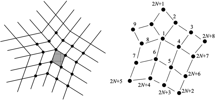
The offline part also includes a subdivision plan data structure created for the face of ground mesh, the data structure including a quadtree for recording the subdivision level and an ordered list of control point templates required to record the face. The quadtree directly reflects the adaptive subdivision of a face. The internal nodes of the quadtree correspond to a recursive subdivision step, and the leaf nodes correspond to subdomains that can be effectively evaluated. Leaf node types include regular nodes, crease nodes, special nodes, and terminal nodes. For the regular face, add all templates of the 16 control points of the face to the template list, and generate conventional nodes corresponding to these templates. In particular, faces with borders or sharp creases are also processed as conventional nodes; Semi-sharp creased faces can be recursively subdivided to eliminate semi-sharp features. For faces with only one half sharp creases, the faces can be directly more efficiently subdivided, and such faces are stored as crease nodes, treated like conventional nodes to process 16 control points, and mark the edge of the crease, record the sharpness with floating point number; If the preset subdivision depth is reached and the face that can be evaluated directly has not been traversed, we need to create a special node. The special node corresponds to an unconventional vertex at the corner of the base mesh face, and the special node corresponds to three templates of the unconventional top, the three templates including the extreme position at the corner and the template of the two tangent lines; For a face without a semi-sharp feature tag, a terminal node is introduced around the unconventional vertex, and the terminal node collapses the n levels of the hierarchy by a fixed 3⁢n regular node or boundary node and a special node. In particular, the special node is a terminal node with n= 0. The terminal nodes store 24 control points per level, distributed over a 5 × 5 mesh. Each terminal node also needs to store a rotation value that specifies the corner of the corresponding unconventional vertex within the parameter domain.

The quadtree maps the u, v locations to subdomains that can be directly evaluated (e.g. regular nodes), and the leaf nodes in the quadtree indirectly reference the required control point templates, each template encoding the control points as weighted sum of one ring vertex, which guarantees the individual use of each template. Use the subdivision plan to store the list of one ring vertices for each face. Since floating point addition is not associated, the calculation of control point values is sensitive to the order of the one ring vertices. When evaluating, each weight must be arranged once to correspond to the ordered list of vertices. We propose to simplify the sorting operation by using the weight adjacency matrix.

The processing of the online part is that each frame of dynamic effects is processed through the pipeline. The online part consists of two processes: the first is to obtain the required sub-control points in the hull shader; the second is to perform curved surface evaluation in the domain shader.

For each control point, we map the scale of the viewport to the minimum subdivision level of the control point through the function n=⌈log2⁡⌈f⌉⌉ (f is the maximum subdivision surface factor of the original surface). Finally, the set of control points for each patch is obtained in the hull shader. At runtime, the original surface settings and tessellation stages are applied to each base mesh face using a hull shader. The hull shader calculates the tessellation factor for edges and interiors and the corresponding control points required for surface evaluation. The segmentation operation then applies the template to the control points required for all n segmentation levels. The subdivision step only calculates the control points, and the topology of subdivided face is stored in the quadtree. Each control point is computed as a convolution of the weights in its template with the one ring vertex of the original surface. In general, you can get the one ring vertices directly in memory, and we improve the performance of the algorithm by using hardware vertex pipeline storage to flatten the cost of the face sharing the vertices. A typical GPU supports 32 vertices as input to the hull shader. When there are more than 32 vertices in one ring vertices, we can also use vertex pipelines. Additional vertices can bypass the vertex shader and get directly from memory.

Surface evaluation is performed in the domain shader. The so-called surface evaluation is to map the control points obtained by the subdivision into vertices in the world coordinate system that can be directly rendered. In the surface evaluation phase, the subdivision plan, the control points output by the hull shader, and the parameter positions of the vertices provided by the hardware subdivision are the inputs, then traverse the quadtree and apply surface evaluation to different nodes with different evaluation methods, finally we get the subdivision surface S⁢(u,v). We traverse the quadtree through an iterative loop and a greedy algorithm. Different traversal methods for different nodes include: (1) for the internal nodes, the traversal is performed until the child node containing the position parameter, and the domain of the corresponding child node is positioned to the position parameter, if the position parameter falls between the child nodes, then we select a child node near the inner side; (2) for a particular node, calculate the final position and normal of the vertex by acquiring the extreme position and tangent control points associated with the node; (3) for the regular nodes, the crease nodes, and the terminal nodes, when traversing to a node that can be directly evaluated, the position and crease data of 16 control points are marked and then directly evaluated using a shader. When traversing to the terminal node, calculate the correct child face (subdomain) with the same logic as directly evaluating.

The evaluation method at the node that can be directly evaluated. Defining initial control vertices of the surface patch through 𝑪0T=(c0,1,…,c0,K) is shown in Fig. 1.

Figure 1.

Evaluate the situation of different nodes.

By subdivision, it generates a set of M=K+9 vertices that are superimposed on the initial vertices. The subset of these new vertices is the control vertices of three uniform B-spline patches. Therefore, three-quarters of the surface patch is parameterized and can be evaluated as a simple bicubic B-spline curve which expressed by vertex sets 𝑪1T=(c1,1,…,c1,K) with 𝑪¯1T=(𝑪1T+c1,K+1,…,c1,M). The lower corner on the left side of the equation represents the sequence number of the patch, the lower corner on the right is labeled 1, ×, 1 and the lower left corner mark have the same meaning, and x is the control point number in the patch. Using these matrices, the subdivision step is multiplied by the K×K ordersubdivision matrix A, i.e. 𝑪1=𝐀𝐂0. The additional point required to evaluate three B-spline patches is to use a larger M×K matrix A¯. Repeat the subdivision step to create an infinite sequence of control vertices 𝑪n=𝐀𝐂n-1=𝑨n⁢𝑪0 and 𝑪¯n=𝑨¯⁢𝑪n-1=𝑨¯⁢𝑨n-1⁢𝑪0,n⩾1. For the subset of the vertices of each level of 𝑪¯n are integrated into the control vertices of the three B-spline patches. These control vertices define 𝑩k,n=𝑷k⁢𝑪¯n,k=1,2,3 according to choosing 16 control vertices from 𝑪¯n. The surface patch corresponding to each matrix of the control vertices can be defined as:

(1)

Sk,n⁢(u,v)=𝑩k,nT⁢b⁢(u,v)=𝑪nT⁢𝑷kT⁢b⁢(u,v)

Where (u,v)∈Ω,n⩾1,k=1,2,3. More formally, the unit square Ω is divided into an infinite patch {Ωkn},n⩾1,k=1,2,3, as shown in Fig. 2. Construct the parameterized subdivision surface for the limited definition of each patch Ωkn through S⁢(u,v):

(2)

S⁢(u,v)|Ωkn=Sk,n⁢(tk,n⁢(u,v))

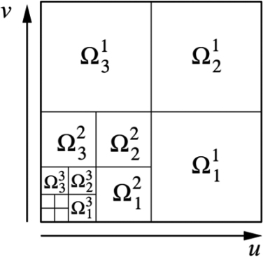
Figure 2.

Fine molecular spatial distribution.

The feature matrix of the subdivision matrix A is defined as a set of eigenvalues and eigenvectors. The feature matrix can be represented as (Λ,V), whereis a diagonal matrix containing the eigenvalues of A, V is an invertible matrix, and each of its columns corresponds to the eigenvector of A. The calculation of the eigenmatrix is equivalent to the solution of the following matrix equation:

(3)

𝐀𝐕=𝐕⁢𝚲

The i-th diagonal element Λ is aneigenvalue of a corresponding eigenvector having an i-th column equal to the matrix 𝑽(i=1,…,K).

The eigenvalues of the subdivision matrix are the eigenvalues of the joint diagonal block, and the eigenvectors of the subdivision matrix should have the form of

𝑽=(𝑼00𝑼1𝑾1).

If the matrix is replaced by their respective blocks Λ and V, we can get the following matrix equation:

(4)

𝑺11⁢𝑼0+𝑺12⁢𝑼1=𝑼1⁢∑

The inverse of the eigenvector matrix is equal to:

(5)

𝑽-1=(𝑼0-10-𝑾1-1⁢𝑼1⁢𝑼0-1𝑾1-1)

Then Eq. (3) can be written as 𝑨=𝑽⁢Λ⁢V-1. This decomposition is a key result for building a surface patch rapid evaluation program. Equation (1) can be written as: Sk,n⁢(u,v)=𝑪^0⁢Λn-1⁢(𝑷k⁢𝐀¯⁢𝑽)T⁢b⁢(u,v). The right side of this equation is independent of the control vertices and the exponent n. Therefore, we can pre-calculate this expression and define the following vectors:

(6)

x⁢(u,v,k)=(𝑷K⁢𝐀¯⁢𝑽)T⁢b⁢(u,v),k=1,2,3

Then the equation for each patch can be expressed as:

(7)

Sk,n⁢(u,v)=𝑪^0⁢Λn-1⁢x⁢(u,v,k),k=1,2,3

Let PiT denote the row of 𝑪0, and the surface patch evaluation can be expressed as:

(8)

S⁢(u,v)|Ωkn=∑i=1K(λi)n-1⁢xi⁢(tk,n⁢(u,v),k)⁢Pi

Bicubic spline function x⁢(u,v,k) can define a set of characteristic basis function for subdivision. For a given eigenvalue λi, define the function φi under the domain Ωkn: φi⁢(u,v)|Ωkn=(λi)n-1⁢xi⁢(tk,n⁢(u,v),k), where i=i,…,K. In the case of the Catmull-Clark subdivision, the characteristic basis function of a particular vertex is a piecewise bicubic polynomial, then Eq. (8) can be expressed as:

(9)

S⁢(u,v)=∑i=1Kφi⁢(u,v)⁢pi

This equation gives surface parameterization corresponding to any face of the control mesh, and Eq. (9) also allows calculation of the surface derivative of random order feature base.

Evaluation of semi-smooth creases. Suppose a patch contains at most one single semi-smooth crease and does not contain any unconventional vertices. The bicubic B-spline patch is evaluated using the tensor product form of the parameters u and v, so a single semi-smooth crease label can be used to simplify the problem to a curved case. The goal is to convert the control points of the cubic B-spline curve to correspond exactly to the half-sharp crease rule of the Catmull-Clark subdivision.

We use the refinement matrix 𝑹¯ (or 𝑹¯P at the boundary of the curve) to improve the cubic B-spline curve. The subdivision of initial curve control point P=(P0,⁢P1,P2,P3)T is expressed as 𝑷¯"=𝑹¯⁢𝑷, 𝑷 is defined as a B-spline control point. Matrix 𝑹¯ and 𝑹¯P correspond to smooth and sharp Catmull-Clark subdivision rules, respectively. Divide Cubic B-spline curve f⁢(t)=N⁢(t)⁢𝑷 into two curves, infinite sharp segment f∞⁢(t) defined on 0⩽t⩽1-2-S and crease transition segment fS⁢(t) defined on 1-2-S<t⩽1, where N⁢(t) is a matrix containing cubic B-spline functions, t is an independent variable, s is the sharpness, when the sharpness is infinity, it is represented by ∞, f⁢(t) represents the cubic B-spline curve function sought. Then control point of two curve segments 𝑷∞ with 𝑷S are obtained for direct evaluation of curves. The speculation curve is defined with control point 𝑷S, which is define in t∈[1-2-S,1] to exactly match the desired parameterized shape corresponding to the initial curve, check if the feature structure of 𝑹 and 𝑹P is full rank, define MS=(R-1)S⁢RPS and diagonalize it and get RPS=VRP⁢𝚲RPS⁢VRP-1 with (𝑹-1)S=𝑽R-1⁢𝚲R-S⁢𝑽R. We can get a simplified 𝑴S (where σ=2S), the role of MS is to convert the input control point to a control point with a sharpness of s.f⁢(t) is given by Eq. (10), the final S⁢(u,v) is determined by Eq. (11).

(10)

f⁢(t)={N⁢(t)⁢𝑴∞⁢𝑷0⩽t⩽1-2-SN⁢(t)⁢𝑴S⁢𝑷1-2-S<t⩽1

(11)

S⁢(u,v)=(f0⁢(u),f1⁢(u),f2⁢(u),f3⁢(u))⁢NT⁢(v)

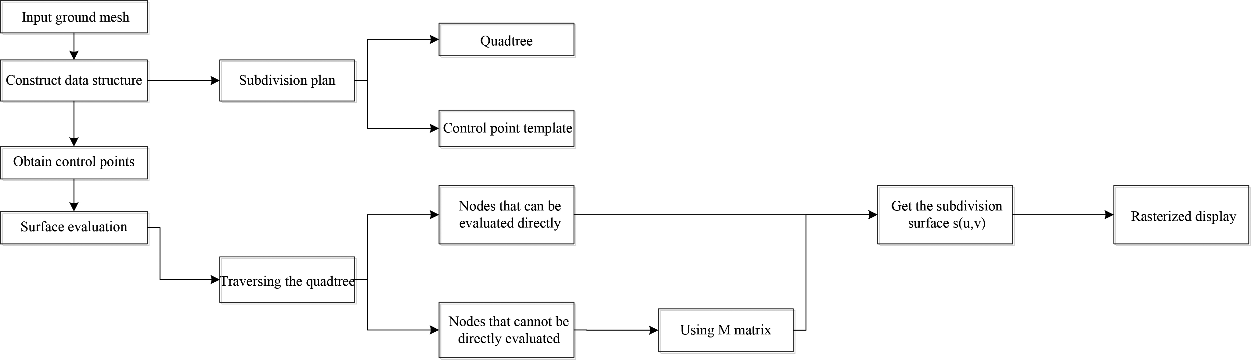
After the surface evaluation, the control points obtained by the subdivision are mapped to the vertices in the world coordinate system that can be directly rendered, and the mapped position and direction are obtained, thereby displaying. Figure 3 is a flow chart of a subdivision rendering algorithm based on surface.

Figure 3.

Flow chart of a subdivision rendering algorithm based on surface.

2.2Solution to the SIMT divergence problem

When traversing a quadtree, there will be a large number of cases where boundaries, creases, or terminal nodes cannot be found. This situation affects the B-spline calculation, making it impossible to filter through the common code path in the sub-domain, causing the Single Instruction Multiple Threads (SIMT) to diverge, as shown in Figs 4 and 5. We construct a complete weighted directed graph based on the quadtrees formed by different subdivision levels. The weights correspond to the changes of the subdivision levels, and then use the greedy algorithm to find the weighted shortest path of any two graph nodes. The method can complete the search for the crease node or the terminal node in the polynomial time, which can improve the search precision and the running speed.

Figure 4.

Example 1 of SIMT divergence.

Figure 5.

Example 2 of SIMT divergence.

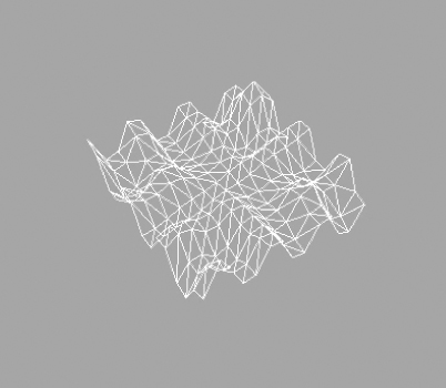
Figure 6.

Frame number curve.

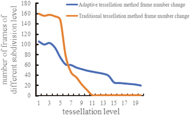
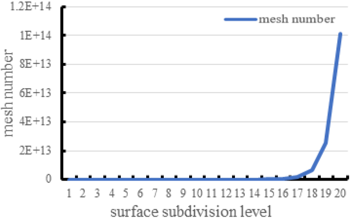
Figure 7.

Mesh number curve.

3.Results and discussion

3.1Speed performance of adaptive tessellation rendering algorithm

We use the classical model (Stanford Bunny) in animation rendering as the speed test model of the surface subdivision-based rendering algorithm. The demonstration mode is a designed loop action, and the mean value of the cyclic frame number is analyzed and processed as the number of frames of different subdivision levels. During the running process of the program, the change of the number of frames is recorded by changing the subdivision level, and the subdivision level 1 to the subdivision level 20 are selected. The speed performance of the tessellation rendering algorithm is tested by analyzing the number of frames displayed at different subdivision levels. The test results are shown in Fig. 6. Subdivision level 1 to subdivision level 4 are periods of overperformance. This is because the hardware performance of the computer can completely handle the number of meshes of these subdivision levels, and better rendering effect can be achieved by hardware acceleration. At this stage, the number of frames of the traditional tessellation algorithm is higher than the adaptive tessellation algorithm proposed in this paper, the reason for this phenomenon is that the basis computational complexity of the adaptive tessellation algorithm is higher than that of the traditional tessellation algorithm, so the traditional tessellation algorithm is better than the adaptive in the lower subdivision level. However, the test results show that the number of frames in both methods is above 100 frames, so the performance difference between the two algorithms does not affect the actual rendering effect. Subdivision level 5 to subdivision level 11 is the performance degradation phase. Since the number of meshes increases by a factor of four for each level of subdivision in the subdivision process, the number of meshes increases exponentially with the increase in the level of the subdivision, as shown in Fig. 7. It can be seen from Fig. 6 that the performance of the traditional tessellation algorithm decreases exponentially with the increase of the subdivision level in the performance degradation stage. When the subdivision level reaches 11, there will be a stutter phenomenon. The performance of the tessellation algorithm decreases linearly with the increase of the subdivision level. When the subdivision level reaches 11, the performance will remain at around 30 frames. Therefore, at this stage, the performance of traditional subdivision algorithms is much lower than that of adaptive subdivision algorithms. Subdivision levels 12 to 20 are periods of insufficient performance. Due to the high level of subdivision at this time, the number of meshes has reached a large number of values and forcing the rendering of so many meshes is prone to program crashes and screen stagnation. In the stage of insufficient performance, the program of the traditional tessellation algorithm is close to collapse, and the picture cannot be upgraded. The number of frames of the adaptive tessellation algorithm decreases linearly. When the subdivision level is 20, it can be maintained at around 30 frames. Therefore, at this stage, the performance of the traditional tessellation algorithm is much lower than that of the adaptive tessellation algorithm. The performance comparison between the traditional tessellation algorithm and the adaptive tessellation algorithm is shown in Table 1.

Table 1

Comparison of performance between traditional tessellation algorithm and adaptive tessellation algorithm

Performance	Traditional tessellation algorithm	Adaptive segmentation algorithm
Initial mesh number	368	368
Basic method of tessellation	Catmull-Clark subdivision surface	Catmull-Clark subdivision surface
Limit breakdown level	11	20
Number of frames in extreme segmentation	Stuck	21

Figure 8.

Subdivision level 1.

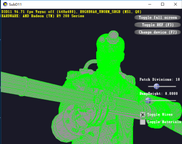
Figure 9.

Subdivision level 10.

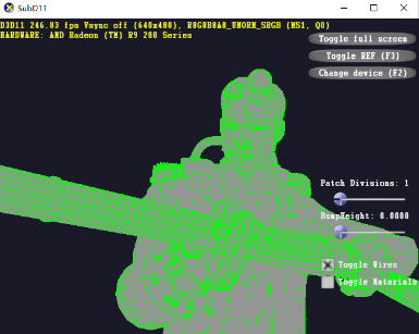
3.2Display performance of adaptive tessellation algorithm

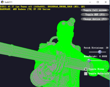
Figure 8 to 11 are display effects of the model at the subdivision level 1, level 10, level 20, and the subdivision level 30, respectively. In this process, as the number of meshes increases, the surface of the model becomes more and more fine and maintains good geometric properties. The display performance rendered using the adaptive tessellation algorithm is compared with the display performance of the Stam algorithm, the PN-triangles algorithm, and the Bezier patch algorithm, which include: subdivision speed, precise boundary of the surface, geometric surface continuity, whether expression attribute values at the edges and the adaptability of special surfaces. The comparison results are shown in Table 2. It can be seen from Table 2 that the adaptive tessellation algorithm is not only superior to other subdivision algorithms in subdivision speed, but also has a wide application range. The subdivided surface geometry properties are not only tangent continuous, but also have continuity of curvature.

Table 2

Tessellation geometry performance

Subdivision algorithm	Subdivision speed	Precisely bounded surface	Continuity	Is there an exact attribute value at the edge?		Whether it is suitable for meshes with boundaries	Whether it is suitable for half sharp creases
				Position	Normal vector
Stam [10]	Slow	√	Second order continuous	×	×	×	×
PN-triangles [2]	Medium	×	Continuous	√	×	√	×
Bezier patch [12]	Medium	×	Continuous	√	×	√	×
Adaptive segmentation algorithm	Fast	√	Second order continuous	√	√	√	√

Figure 10.

Subdivision level 20.

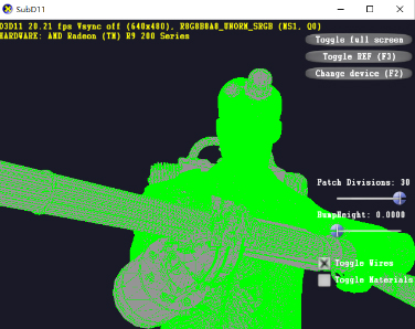
Figure 11.

Subdivision level 30.

3.3Computational performance of adaptive tessellation rendering algorithm

Sharma and Batra propose to use the real root isolation algorithm to improve the running time of the subdivision algorithm. The basic operation of tessellation is O(logn), they use the Newton graph to calculate O(n) in each iteration, and use Taylor displacement O(nlogn) performs approximate calculation, and the time complexity of using the algorithm to implement tessellation is O⁢(n2⁢log⁡σ). and σ<1 [22].

The tessellation algorithm proposed in this paper is related to the basic operation amount O(logn) of traversing the quadtree in terms of time complexity, and also depends on the running time of traversing the quadtree. We greatly reduce the time complexity by using the greedy algorithm. The algorithm is related to the three operations Insert, Extract_Min, and Decrease_key in the Fibonacci heap. In the Fibonacci heap, Extract_Min’s amortization time is O(lgV), and Decrease_ key’s amortization time is O(1). So the running time of the algorithm includes: line 1-3O(|G.V|), line 4O(1), line 5O(1), line 6O(|G.V|), line 7 of loops, line 8 of running time O(G.VlgG.V), line 9 running time O(G.V), the total running time in a 10-line cycle is O(G.E).The optimized total running time is only O(VlgV+E), while the running time before timization is exponential. In summary, when the subdivision level is low, the time complexity of the adaptive tessellation algorithm is O⁢(n⁢(log⁡n)2), the time complexity is higher when the subdivision level is higher O⁢(n2⁢log⁡n). Therefore, the performance of the adaptive tessellation algorithm is better than the time complexity of the Sharma and Batra algorithms when the subdivision level is low.

Figure 12.

Basic operation flow of soft tissue rendering in virtual surgery system.

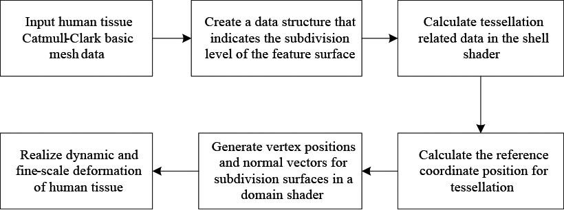
Figure 13.

Subdivision level 1 thigh rendering effect.

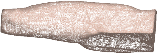
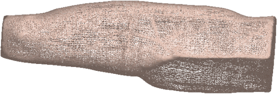
Figure 14.

Subdivision level 10 thigh rendering effect.

3.4Application of adaptive tessellation algorithm in soft tissue model rendering of virtual surgery system

The steps of applying the adaptive tessellation algorithm to the virtual surgery soft tissue model include: (1) reading the muscle model information including the topological relationship of each vertex, the characteristic label, and the vertex position. Input this data information into the vertex shader and process the vertices into surfaces in the vertex shader. (2) Create a data structure for each sub-surface that indicates the subdivision level of the feature surface. This data structure includes a quadtree structure that reflects the tessellation hierarchy and an ordered list of control point templates for tessellation. (3) In the subdivision stage, use the hull shader to calculate the edge of each base mesh sub-surface, the internal surface subdivision factor and the control points required for tessellation. The specific steps include defining the rendering using OpenGL library functions. Each patch input of the pipeline consists of 16 vertices. Then the control points of each subdivision surface are calculated by a recursive algorithm, and the control point information is stored in the corresponding nodes of the quadtree, and the tessellation level is recorded. Each recursion produces a subdivision hierarchy, and we use the internal node (I) to record each recursive hierarchy generated. When the recursive subdivision produces a regular surface, the template of the 16 control points corresponding to the regular surface is added to the template list and generate the regular nodes (R) of these templates. The R node is stored in the frame buffer, and X, Y, and Z store three components of the control point position, and N stores the normal vector. If the traversal reaches the set subdivision depth but does not reach the sub-surface corresponding to the final position, then a special node (E) is created, which corresponds to the corner of the base mesh surface and is a special vertex (EV). We calculate the template at the extreme position of the corner and the two tangent lines and add them to the template list. For each subdivision level, the established quadtree has three regular nodes and one internal node and establishes a terminal node (T) at the highest level, indicating that the subdivision is terminated. The template is used to encode the control points as the weighted sum of the vertices of the one ring neighborhood, and the template is represented by a weighted array. The one ring neighborhood vertex can be directly read in memory, and a 16*16 matrix is used to store the weights of all one ring vertices in order to record the topological relationship between the vertices and the correspondence between the weights and the control points. The weights corresponding to the one ring vertex and its control points are read from the weight relationship matrix, and their convolutions are calculated to obtain the reference position of the subdivided vertices. (4) In the domain shader, we will traverse the quadtree to get the position of the control point, the normal vector and the vertex reference position of the hull shader output as input, and the final renderable vertex position, normal vector and the topological relationship of all vertices. Find all child nodes by traversing the internal nodes. When the traversed child node is an R node, the control point position and the normal vector are output, and the domain shader maps to the final renderable vertex position and normal vector. When the traversed child node is an E node, the domain shader directly outputs the control point position and the normal vector. The traversal is terminated when the child node traversed is a T node. The basic operation flow of the adaptive tessellation rendering algorithm applied to the soft tissue rendering of the virtual surgery system is shown in Fig. 12. Figures 13 and 14 show the thigh rendering effects of subdivision level 1 and subdivision level 10, respectively. The proposed adaptive tessellation rendering algorithm in this paper aims to have improved performance in the aspects of display, computation, and speed compared to the traditional tessellation algorithm.

4.Conclusion

This paper proposes an adaptive tessellation rendering algorithm, which uses the quadtree to record the surface subdivision hierarchy and uses the control template to record the control point information to simplify the complex surface subdivision steps. The algorithm uses a matrix to record topological relationships and vertex weights between vertices, reducing computation time. The algorithm associates the quadtree of each subdivision level by the graph algorithm and uses the greedy algorithm to compress the time complexity of traversing different subdivision levels of the quadtree to O(nlogn). The adaptive tessellation rendering algorithm proposed in this paper is compared with the traditional tessellation algorithm and the current excellent tessellation algorithm. The proposed algorithm has advantages in display performance, computational performance and speed performance when the subdivision level is high. Applying the adaptive tessellation rendering algorithm to the real-time rendering of soft tissue of virtual surgery system, while rendering excellent solid animation, it also greatly improves the response speed of virtual surgery system calculation and rendering.

Acknowledgments

This research was supported by NSFC (No. 61972117).

Conflict of interest

None to report.

References

[1]	Doo D, Sabin M. Behaviour of recursive division surfaces near extraordinary points. Computer-Aided Design. (1978) ; 10: (6): 356-360.
[2]	Loop CT. Smooth Subdivision Surfaces Based on Triangles. Department of Mathematics the University of Utah Masters Thesis, (1987) .
[3]	Nasri AH. Polyhedral subdivision methods for free-form surfaces. Acm Transactions on Graphics. (1987) ; 6: (1): 29-73.
[4]	Hoppe H, Derose T, Duchamp T, et al. Piecewise smooth surface reconstruction,Conference on Computer Graphics and Interactive Techniques. ACM. (1994) : 295-302.
[5]	Derose T, Kass M, Truong T. Subdivision surfaces in character animation. Conference on Computer Graphics and Interactive Techniques. ACM. (1998) : 85-94.
[6]	Forsey DR, Bartels RH. Hierarchical B-spline refinement. ACM. (1988) : 205-212.
[7]	Cook RL, Carpenter L, Catmull E. The Reyes image rendering architecture. AcmSiggraph Computer Graphics. (1987) ; 21: (4): 95-102.
[8]	Schäfer H, Raab J, Keinert B, et al. Dynamic feature-adaptive subdivision. I3D. 2015: : 31-38.
[9]	Keinert B, Fisher M, Stamminger M, et al. Real-Time Rendering Techniques with Hardware Tessellation. Computer Graphics Forum. (2016) ; 35: (1): 113-137.
[10]	Stam J. Exact evaluation of Catmull-Clark subdivision surfaces at arbitrary parameter values. (1998) : 395-404.
[11]	Bolz J, Der P. Rapid evaluation of Catmull-Clark subdivision surfaces. International Conference on 3d Web Technology. DBLP. (2002) : 11-17.
[12]	Loop C, Schaefer S. Approximating Catmull-Clark subdivision surfaces with bicubic patches. Acm Transactions on Graphics. (2008) ; 27: (1): 1-11.
[13]	Myles A, Yeo YI, Peters J. GPU conversion of quad meshes to smooth surfaces. Spm Proceedings of the Acm Symposium on Solid & Physical Modeling. (2008) ; 321-326.
[14]	Ni T, Yeo Y, Myles A, et al. GPU smoothing of quad meshes. IEEE International Conference on Shape Modeling and Applications. IEEE. (2008) : 3-9.
[15]	Myles A, Ni T, Peters J. Fast parallel construction of smooth surfaces from meshes with tri/quad/pent facets. Symposium on Geometry Processing. Eurographics Association. (2008) : 1365-1372.
[16]	Loop C, Schaefer S, Ni T. Approximating subdivision surfaces with Gregory patches for hardware tessellation. ACM. (2009) : 1-9.
[17]	He L, Loop C, Schaefer S. Improving the Parameterization of Approximate Subdivision Surfaces. Computer Graphics Forum. (2013) ; 31: (7): 2127-2134.
[18]	Kovacs D, Mitchell J, Drone S, et al. Real-time creased approximate subdivision surfaces. Symposium on Interactive 3d Graphics and Games. ACM. 2009: : 155-160.
[19]	Schäfer H, Raab J, Keinert B, et al. Dynamic feature-adaptive subdivision. I3D. (2015) : 31-38.
[20]	Fu HH, Yang HM, Chen CY. Large-scale terrain-adaptive LOD control based on GPU tessellation. Alexandria Engineering Journal. (2021) : 2865-2874.
[21]	Zhang LW, She JF, Tan JZ, et al. A Multilevel Terrain Rendering Method Based on Dynamic Stitching Strips. Isprs International Journal of Geo-Information. (2019) ; 8: (6).
[22]	Sharma V, Batra P. Near optimal subdivision algorithms for real root isolation. Journal of Symbolic Computation. (2015) : 331-338.