
Verification of temperature, wind and precipitation fields for the high-resolution WRF NMM model over the complex terrain of Montenegro
Abstract
BACKGROUND:
The necessity of setting up high-resolution models is essential to timely forecast dangerous meteorological phenomena.
OBJECTIVE:
This study presents a verification of the numerical Weather Research and Forecasting non-hydrostatic Mesoscale Model (WRF NMM) for weather prediction using the High-Performance Computing (HPC) cluster over the complex relief of Montenegro.
METHODS:
Verification was performed comparing WRF NMM predicted values and measured values for temperature, wind and precipitation for six Montenegrin weather stations in a five-year period using statistical parameters. The difficult task of adjusting the model over the complex Montenegrin terrain is caused by a rapid altitude change in in the coastal area, numerous karst fields, basins, river valleys and canyons, large areas of artificial lakes on a relatively small terrain.
RESULTS:
Based on the obtained verification results, the results of the model vary during time of day, the season of the year, the altitude of the station for which the model results were verified, as well as the surrounding relief for them. The results show the best performance in the central region and show deviations for some metrological measures in some periods of the year.
CONCLUSION:
This study can give recommendations on how to adapt a numerical model to a real situation in order to produce better weather forecast for the public.
1.Introduction
The atmosphere represents deterministic chaos, in which various processes in space and time in different resolutions interact both with each other and with boundary surfaces, i.e. oceans and land of various physical characteristics. The behavior of the atmosphere with various processes predominantly influenced by the activity of the Sun, the rotation of the Earth, the state of the soil, etc. it is very difficult to explain and forecast.
The invention of the computer in the fifties of the last century and the enabling of a large number of calculation operations in a short period of time enabled numerical forecasting to begin a new era of meteorological science and practice. The first successful numerical weather forecast was calculated on ENIAC, the first digital computer, with a team of meteorologists headed by the American meteorologist Jule Charney [1]. Unsolvable nonlinear differential equations became possible to approximate with a series of numerical methods. Larger regional models, which were very expensive in terms of necessary computer performance and time in previous decades, became available in last decade using modern distributed computing resources and applicable to larger areas with larger horizontal and vertical resolution. A big challenge for weather forecast modeling is the adjustment of steps in time and space, the choice of parameterization schemes of regional numerical models, in order to obtain a more accurate forecast for the area of interest. With a coarse resolution on a complex terrain such as Montenegro, it is hard to monitor mesoscale and microscale processes such as hail, summer convection accompanied by showers, locally strong gusts of wind, inversion that causes an increase in pollution in urban settlements, as well as to precisely determine the area affected by precipitation and its amount, intensity, start and end time. On the other hand, high-resolution models under unstable conditions can calculate unrealistically high values of pressure gradients, local wind gusts, and precipitation amounts, but they certainly increase the chance of successful forecasting of dangerous meso- and micro-scale weather processes.
The Weather Research and Forecasting (WRF) model [2, 3] has been used in arid regions for various forecasting and verification purposes [4, 5, 6, 7, 8] and process studies [9, 10, 11, 12, 13]. The Weather Research and Forecasting non-hydrostatic Mesoscale Model (WRF NMM) is a fully compressible model for mesoscale weather systems, non-hydrostatic but with a hydrostatic option [14, 15, 16]. The model uses a hybrid sigma coordinate, while the distribution of calculation points is on Araka’s E-grid.
The complex terrain on which Montenegro is located represents a great challenge for successful meso-scale weather forecasting. Meteorological stations from which data were collected for WRF NMM verification are located in various geographical areas with different relief features, so the verification results will objectively show for which type of relief and geographical coordinates, the model shows more and for which less successful forecasts of tendencies of basic meteorological quantities.
In the following chapters, by comparing the observed and modeled values for each of the stations, objective evaluations of the forecast will be determined via mean difference (MD), mean absolute difference (MAD) and root mean square difference (RMSD), at the level of months and time of day using dataset obtained during five years. Contingency tables will be used to verify the precipitation field [17]. Based on the obtained results, the performance of the WRF NMM model over the complex terrain of Montenegro, which is used by the National Meteorological Service for operational purposes, will be discussed.
Used numerical models were verified over the Mediterranean [18, 19], but also over the complex terrains of the UAE [20] and mountainous regions [21]. This paper is the first research on the complex terrain of Montenegro.
2.Materials and methods
The subject of the research are meteorological measuring stations in the cities of Bar, Žabljak, Nikšić, Pljevlja, as well as the Golubovci (near Podgorica) and Tivat airports (Fig. 1). The data sources used in this analysys are eight-hour data reports, so-called sinop reports. By decoding, filtering and sorting them, a database of eight-hour meteorological quantities was created, which will be used during verification for each of the stations.
Table 1
Synoptic stations. Name with latitude, longitude, WMO number, model and true elevation
| Station | Latitude | Longitude | WMO number | Model elevation | Elevation |
|---|---|---|---|---|---|
| Bar | 42.100 | 19.083 | 13461 | 4 | 6 |
| Golubovci (LYPG) | 42.359 | 19.252 | 13462 | 54 | 33 |
| Niksic | 42.766 | 18.952 | 13459 | 651 | 647 |
| Pljevlja | 43.350 | 19.350 | 13363 | 846 | 784 |
| Tivat (LYTV) | 42.404 | 18.723 | 13457 | 73 | 5 |
| Zabljak | 43.150 | 19.120 | 13361 | 1423 | 1450 |
Figure 1.
The domain of the WRF NMM model (red square) and the geographical location of the stations on the map of Montenegro.
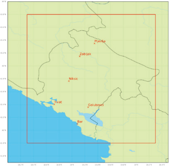
Table 1 presents the measuring stations, sources of observation, their coordinates, WMO number, altitude in the model and actual altitude. The preliminary cause of the error in the modelled values lies in the fact that the actual altitude is different from that used by the numerical model as orography.
After obtaining prognostic meteorological parameters for 24 hours in advance, a database of hourly modelled and eight-hour temperature values at a height of 2 m and wind speed at a height of 10 m was created, while precipitation was summarized in twelve-hour intervals, i.e. from 6 a.m. to 6 p.m. and from 6 p.m. until 6 a.m. the next day. The time frame on which data was collected for further processing is 5 years, i.e. from 2017 to 2021.
In our case, the time step of the numerical model is 3 s and in space dx
The differences representing the objective statistical evaluations of the forecast are calculated according to the formulas:
1. Mean Difference (MD) or bias is defined as the sum of the difference between forecasted (F) and observed (O) values divided by the total number of samples.
2. Mean Absolute Difference (MAD) is the ratio between the sum of the absolute value of the difference between observations (O) and forecasts (F) and the total number of samples.
3. The Root Mean Squared Difference (RMSD) is more sensitive to larger errors than the MAD.
Whether the mean difference is greater or less than zero depends on whether the model underestimates or overestimates the observations. RMSD gives us information about the intensity of the error. The forecast has better performance if the RMSD value is smaller and the MD is close to zero. The correlation coefficient is another measure of forecast accuracy and reflects the linear relationship between forecasts and observations.
The binary contingency table consists of the following matrix:
| Observed | |||
|---|---|---|---|
| Observed no | Observed yes | ||
| Forecasted | Forecasted no | fp | fn |
| Forecasted yes | tn | tp | |
tp (true positive) or hits are those events that were forecasted and actually occurred; tn (true negative) or correct negatives are the events that were not forecasted and did not occur; fp (false positive) or false alarms are those events that were forecasted but not occur; fn (false negative) or misses are the events occurred but not forecasted.
Accuracy, or fraction correct, is the ratio between the sum of hits and correct negatives and the N_total. It can assume values ranging from 0 to 1 (best value). Accuracy gives the fraction of the overall correct forecasts.
Bias score, also called frequency bias, measures the ratio of the frequency of forecasts to the frequency of observations. Can assume values over zero (perfect score is 1). If BIAS
3.Results and discussion
The mean, mean absolute and root mean square difference for the temperature are shown in Fig. 2.
Regular daily trends of the mean difference for cities in the southern (Bar and Tivat) and northern (Žabljak and Pljevlja) regions are noticeable. Early morning and evening hours are characterized by a negative difference and midday by a positive difference, which will be noticeable and explained in more detail below (Fig. 4). The intensity of the error, represented by RMSD, is the highest in the coastal region and it is 5.4
The central region (Nikšić and Golubovci) do not have such a clearly expressed amplitude of the mean difference. For both stations, the RMSD values are higher in the evening and early morning hours than in the midday hours. In terms of intensity, the maximums are lower than other stations, and amount to 2.9
The seasonal course of the statistical quantitative verification scores is presented in Fig. 2. The RMSD for Bar has a regular seasonal course with a maximum in the month of June (equal to 4.5
The most interesting RMSD difference is noticeable for Žabljak. The highest RMSD value for the mentioned station was reached in April and is 4.9
Nikšić and Golubovci has higher RMSD values in the winter and lower values in the summer months. By the intensity of the maximum, which is 2.5
Figure 4 shows us visually how the model behaves during periods of day (left figure) and during months (right figure), based on the MD value. The blue shade indicates how cold the model is (i.e. how much the model underestimates), and the red how warm the model is (i.e. overestimates).
The largest positive mean difference at the daily level, typical for Bar, is at noon. Also at the same time of day for Tivat, with a noticeable stronger shade of red in the early morning and evening hours, which
Figure 2.
Variations of (blue) mean difference, (blue) mean absolute difference and (red) root mean square difference (
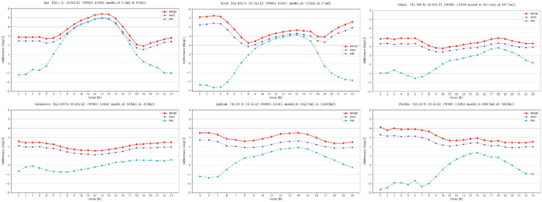
Figure 3.
Variations of (yellow) mean difference, (green) mean absolute difference and (brown) root mean square difference (
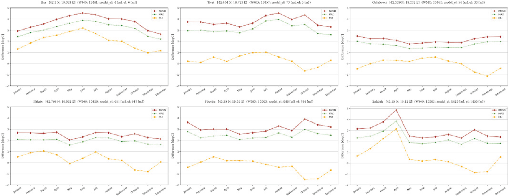
Figure 4.
Heatmap of mean difference. Shades of blue means underestimation of model while the red shade shows overestimation of modelled temperature.
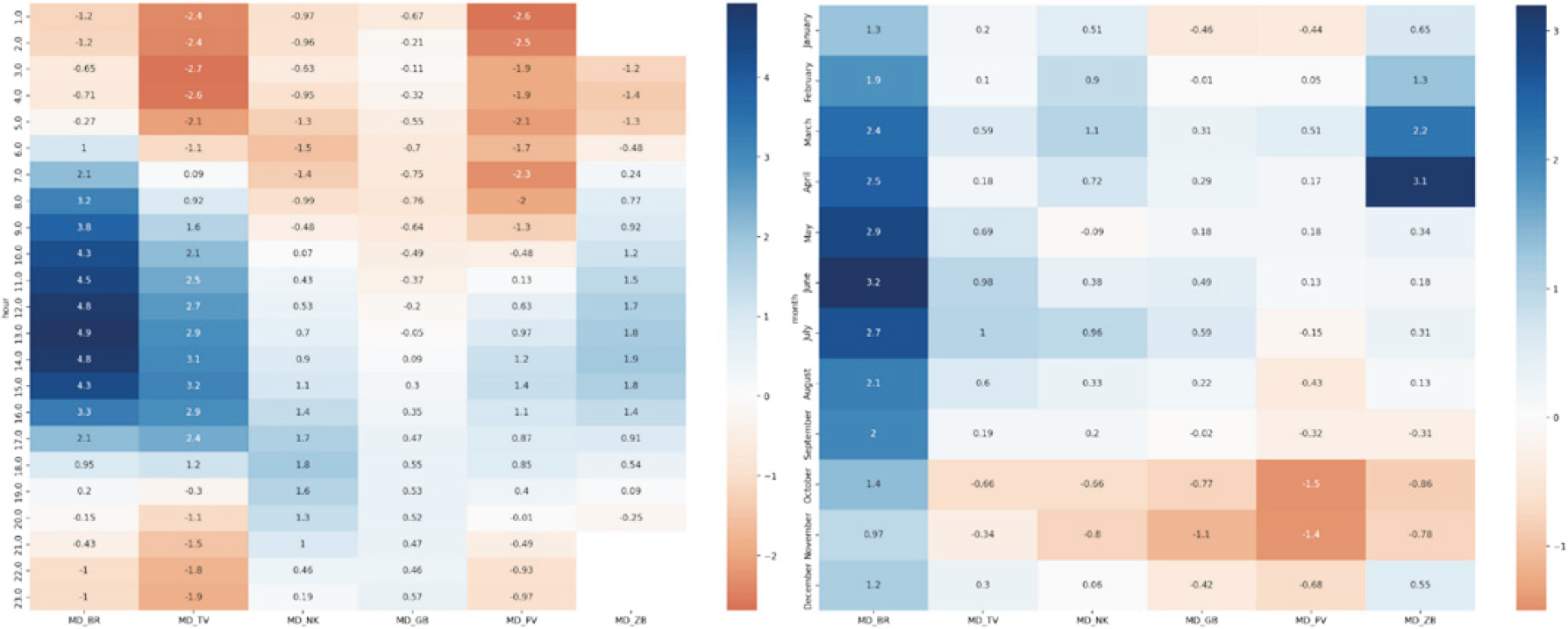
indicates a great contrast, i.e. poor performance. For Nikšić and Golubovci, the lighter shade of both colours indicates better performance of the model.
In Fig. 4 on the right, there is a noticeable underestimation of the model for all months for the Bar station, a stronger blue shade for Žabljak in April and a stronger reddish shade in Pljevlja in October and November.
Figure 5 presents graphs in the form of points (scatterplot) for each of the cities with observed temperature intensity on the h-axis and modeled on the u-axis.
The highest correlation coefficients with values of 0.97 and 0.96 were recorded for the station Golubovci and Nikšić respectively. On the other hand, the lowest correlation coefficients are for Tivat and Bar stations, with values of 0.89 and 0.9, respectively.
In Fig. 6 presents the values of the verification ratings, for the wind field, for each of the stations for each of the hours during the day.
Southern stations in the coastal region (Tivat and Bar) have a regular daily course of the mean difference with minimum values in the morning and evening and maximum in the midday hours. For the other stations, with the exception of Pljevlja (before dawn and in the late evening hours), they have negative mean difference values, i.e. the model overestimates the observed values.
The intensity of the error, expressed through the RMSD score, reaches its peak in the midday hours in Golubovci and Pljevlja, while at the other stations, the peaks, i.e. the biggest model errors were recorded in the early morning and evening hours.
In terms of intensity, the errors are noticeably larger for coastal stations and Žabljak. Thus, the RMSD values are the highest for Bar, Žabljak and Tivat and amount to 5.49 ms
The seasonal trend of the model verification statistics for each of the observed stations is shown in Fig. 7. With the exception of Bar from April to September, all other stations have a negative mean difference, i.e. the model overestimates wind speeds in all months. Each of the stations, in the winter months has the RMSD with maximum values. The best performance of the model, observed in relation to the lowest intensity of maximum RMSD values, is for Pljevlja, Golubovci and Tivat and amounts to 2.9 ms
The maximum RMSD was reached for every city in February, except for Žabljak when it was reached in December.
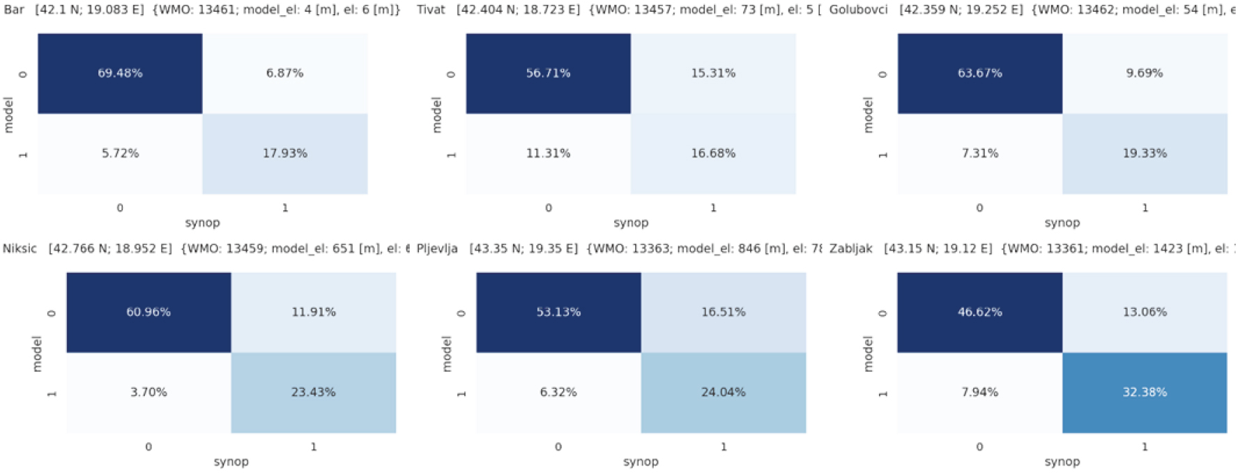
Precipitation in the synop dispatches is available at 6 and 18 UTC. The model forecasts the precipitation in these intervals in order to bring them to the same reference plane for observation. Figure 8 presents the contingency matrices. Zeros and ones indicate whether precipitation did not or did occur in the same intervals, for the synopsis on the h-axis and the model on the u-axis. BS for all stations does not exceed the value of 1, which means that the model underestimates precipitation.
Accuracies are 87.4%, 73.4%, 83%, 84.4%, 77.2%, 79%, for Bar, Tivat, Golubovci, Niksic, Pljevlja, Zabljak respectively. It means that the best accuracy is for Bar and the lowest is for Tivat.
The BS values are 0.95, 0.92, 0.89, 0.87, 0.77, 0.74 for Bar, Golubovci, Žabljak, Tivat, Nikšić and Pljevlja, respectively. Based on the above, we conclude that as far as the precipitation field is concerned, the model shows the best performance for Bar, and the worst for Pljevlja.
Figure 5.
Correlation coefficient (CC) of the WRF NMM temperature forecast against temperature observations for forecasting periods of 24, 48 and 72 hours.
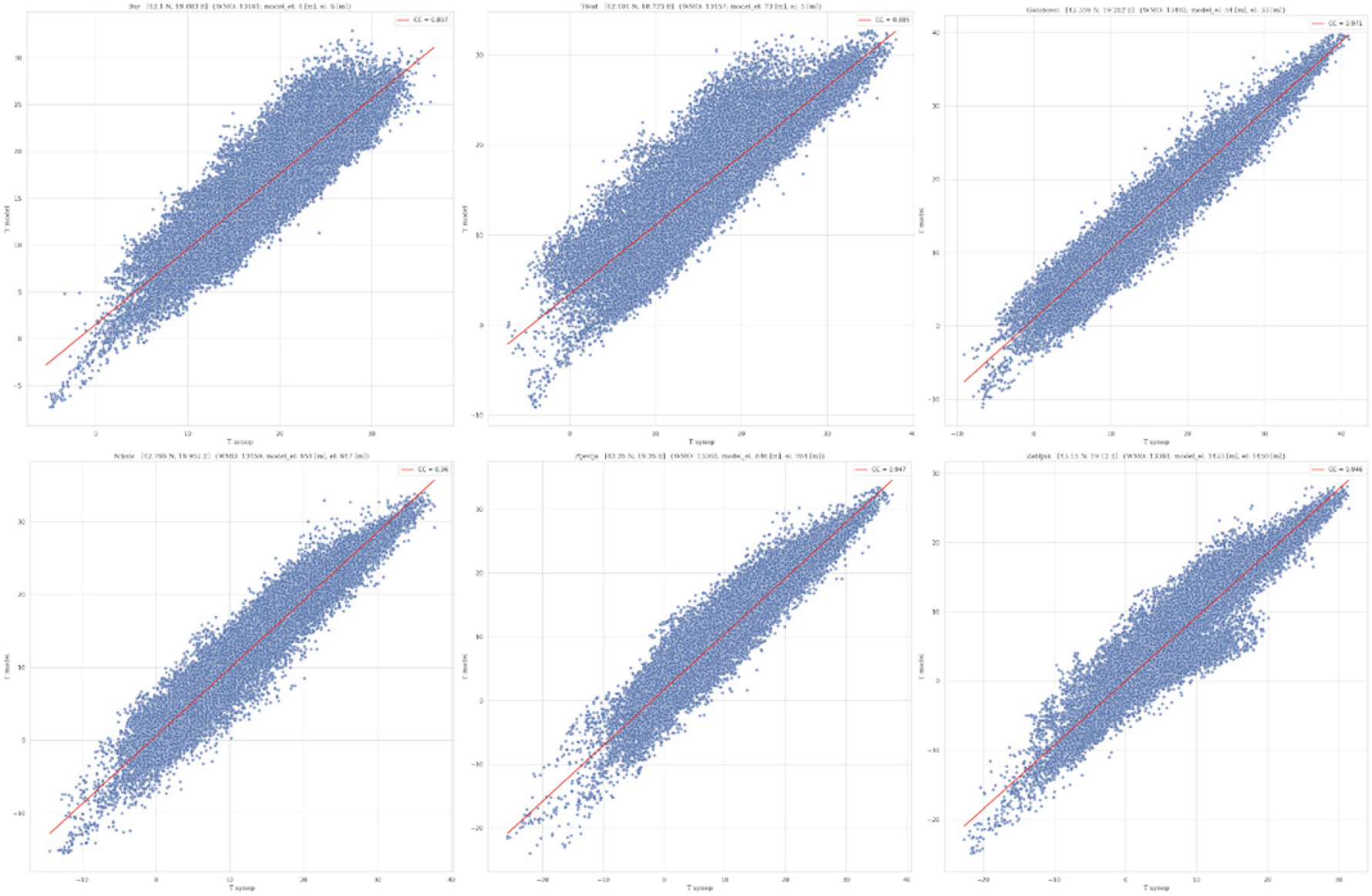
Figure 6.
Variations of mean difference(dark grey), mean absolute difference (grey) and root mean square difference (light grey) of the NMM WRF model forecast against wind on the 10 m observations during a day. x axis is time in hours (UTC).
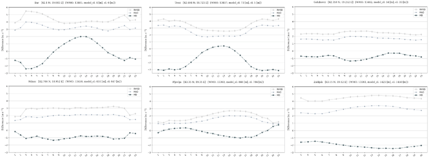
Figure 7.
Variations of (dark blue) mean difference, (blue) mean absolute difference and (light blue) root mean square difference (ms
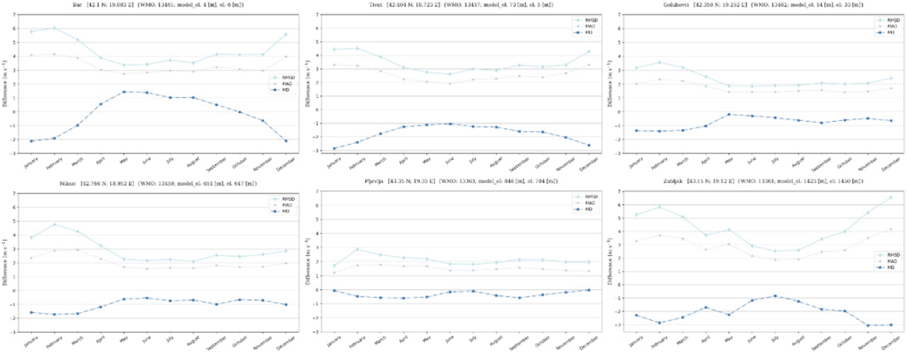
Figure 8.
Binary contingency tables (it is best to remove them, leaving only the results).
4.Conclusion
The necessity of setting up high-resolution models is essential to timely forecast dangerous meteorological phenomena. The difficult task of adjusting the model over the complex Montenegrin terrain is caused by a rapid altitude change in in the coastal area, numerous karst fields, basins, river valleys and canyons, large areas of artificial lakes on a relatively small terrain.
Based on the obtained verification results, we conclude that for the basic meteorological parameters of temperature, wind and precipitation, the performance of the model will depend on the time of day, the season of the year, the altitude of the station for which the model results were verified, as well as the surrounding relief for them.
For temperature, as one of the basic meteorological quantities and the most important quantity for the public, the high resolution WRF NMM model, it was determined that the model shows the weakest performance for Bar and Žabljak, while it is the most reliable for Golubovci. The most significant error is for the month of April for Žabljak with a value of 4.9
The wind field is in all cases, if the mean difference is observed for the months of the year, except for Bar from April to September, overestimated by the model. The intensity of the error is usually higher in the winter months than in the rest of the year. Based on the intensity of errors based on hourly values during the day and monthly values during the year, we conclude that the model better forecasts the wind field for Golubovci compared to other stations, and one of the reasons lies in the fact that the surrounding relief is homogeneous in a wider area for the mentioned station in relation to the others.
With the contingency matrices, the values in percentages of coincidence of precipitation detection with the model and synop dispatch in two intervals at 6 and 18 UTC were determined, as well as the percentages when there was no coincidence. Using the formula for BS, it was determined that for all stations the model underestimates the precipitation values. The worst performances are for Pljevlja, and the best for Bar.
Potential topics for further research are the large value of error when forecasting the temperature in April for Žabljak, Pljevlja for October and September, as well as the consistently cold model for all months of the year for Bar.
Improved computing performances allows us to run a number of numerical models with slightly disturbed initial fields and different settings of physics and parameterization numerical model schemes, obtaining the so-called ensemble of models, and the national hydro-meteorological services, which with the help of a series of indices [25] would better forecast dangerous meteorological phenomena and the service for emergency situations as well as the local population would be better prepared for potential dangers.
Conflict of interest
None to report.
Funding
This research was partially funded by the EUROCC project, European High-Performance Computing Joint Undertaking (JU) under grant agreement no. 951732. The JU received support from the European Union’s Horizon 2020 research and innovation programme and EUROCC project participating institutions.
References
[1] | Weik MH. The ENIAC Story. Ordnance. Washington, DC: American Ordnance Association (January–February (1961) ). |
[2] | J G. Powerset all, “The Weather Research and Forecasting (WRF) Model: Overview, System Efforts, and Future Directions”, Bulletin of the American Meteorological Society, 10.1175/BAMS-D-15-00308.1 |
[3] | Skamarock WC, Klemp JB, Dudhia J, Gill DO, Barker D, Duda MG, Powers JG. A Description of the Advanced Research WRF Version 3 (No. NCAR/TN-475+STR). University Corporation for Atmospheric Research. (2008) . doi: 10.5065/D68S4MVH. |
[4] | Branch O, Warrach-Sagi K, Wulfmeyer V, Cohen S. Simulation of semi-arid biomass plantations and irrigation using the WRF-NOAH model – A comparison with observations from Israel. Hydrology and Earth System Sciences. (2014) ; 18: : 1761–1783. doi: 10.5194/hess-18-1761-2014. |
[5] | Fonseca R, Temimi M, Thota MS, Nelli NR, Weston MJ, Suzuki K, Uchida J, Kumar KN, Branch O, Wehbe Y, et al. On the analysis of the performance of WRF and NICAM in a hyperarid environment. Weather Forecast. (2020) ; 35: : 891–919. |
[6] | Thomas S, et al. Near-global-scale high-resolution seasonal simulations with WRF-Noah-MP v.3.8.1. Geosci. Model Dev. (2020) ; 13: : 1959–1974. doi: 10.5194/gmd-13-1959-2020. |
[7] | Valappil VK, Temimi M, Weston M, Fonseca R, Nelli NR, Thota M, Kumar KN. Assessing Bias Correc-tion Methods in Support of Operational Weather Forecast inArid Environment, Asia-Pacific J. Atmos. Sci. (2020) ; 56: : 333–347. doi: 10.1007/s13143-019-00139-4. |
[8] | Wehbe Y, Temimi M, Weston M, Chaouch N, Branch O, Schwitalla T, Wulfmeyer V, Zhan X, Liu J, Al Mandous A. Analysis of an extreme weather event ina hyper-arid region using WRF-Hydro coupling, station, andsatellite data. Nat. Hazards Earth Syst. Sci. (2019) ; 19: : 1129–1149. doi: 10.5194/nhess-19-1129-2019. |
[9] | Becker K, Wulfmeyer V, Berger T, Gebel J, Münch W. Carbon farming in hot, dry coastal areas: An option forclimate change mitigation. Earth Syst. Dynam. (2013) ; 4: : 237–251. doi: 10.5194/esd-4-237-2013. |
[10] | Branch O, Wulfmeyer V. Deliberate enhancement of rainfallusing desert plantations. P. Natl. Acad. Sci. USA. (2019) ; 116: : 18841–18847. doi: 10.1073/pnas.1904754116. |
[11] | Karagulian F, Temimi M, Ghebreyesus D, Weston M, Kon-dapalli NK, Valappil VK, Aldababesh A, Lyapustin A, Chaouch N, Al Hammadi F, Al Abdooli A. Anal-ysis of a severe dust storm and its impact on air qualityconditions using WRF-Chem modeling, satellite imagery, andground observations. Air Qual. Atmos. Heal. (2019) ; 12: : 453–470. doi: 10.1007/s11869-019-00674-z. |
[12] | Nelli NR, Temimi M, Fonseca RM, Weston MJ, Thota MS, Valappil VK, Branch O, Wulfmeyer V, Wehbe Y, Al Hosary T, Shalaby A, Al Shamsi N, Al Naqbi H. Impact of Roughness Length on WRF Simulated Land-Atmosphere Interactions Over a Hyper-Arid Region. Earth Sp. Sci. (2020) a; 7: : e2020EA001165. doi: 10.1029/2020ea001165. |
[13] | Wulfmeyer V, Branch O, Warrach-Sagi K, Bauer HS, Schwitalla T, Becker K. The impact of plantations onweather and climate in coastal desert regions. J. Appl. Meteorol. Climatol. (2014) ; 53: : 1143–1169. doi: 10.1175/JAMC-D-13-0208.1. |
[14] | Janjic Z. A nonhydrostatic model based on a new approach. Meteorol Atmos Phys. (2003) ; 82: : 271–285. doi: 10.1007/s00703-001-0587-6. |
[15] | Janjić ZI. A non-hydrostatic model based on a new approach. Meteorology and Atmospheric Physics. (2003) a; 82: : 271–285. |
[16] | Janjić ZI. The NCEP WRF Core and Further Development of Its Physical Package. 5th. International SRNWP Workshop on Non-Hydrostatic Modeling. Bad Orb, Germany, 27–29 October, (2003) b. |
[17] | Wilks DS. Statistical Methods in the Atmospheric Sciences, Academic Press, (1995) ; 233–242. |
[18] | Papadopoulos A, Katsafados P. Verification of operational weather forecasts from the POSEIDON system across the Eastern Mediterranean. Nat. Hazards Earth Syst. Sci. (2009) ; 9: : 1299–1306. doi: 10.5194/nhess-9-1299-2009. |
[19] | Petros Katsafados, 12th Annual WRF Users’ Event, 20–24 June (2011) , Boulder CO, USA. |
[20] | Branch O, Schwitalla T, Temimi M, Fonseca R, Nelli N, Weston M, Milovac J, Wulfmeyer V. Seasonal and diurnal performance of daily forecasts with WRF V3.8.1 over the United Arab Emirates. Geosci. Model Dev. (2021) ; 14: : 1615–1637. doi: 10.5194/gmd-14-1615-2021. |
[21] | Roux G, Liu Y, Delle Monache L, Sheu R-S, Warner T. Verification of high resolution wrf-rtfdda surface forecasts over mountains and plains, NCAR/Research Application Laboratory. (2009) . |
[22] | Rogers E, Black TL, Deaven DG, DiMego GJ, Zhao Q, Baldwin M, Junker N, Lin Y. Changes to the operational ‘early’ Eta Analysis/Forecast System at the National Centers for Environmental Prediction. Weather Forecast. (1996) ; 11: : 391–413. |
[23] | Fels SB, Schwarzkopf MD. An efficient, accurate algorithm for calculating CO215 μm band cooling rates. Journal of Geophysical Research. (1981) ; 86: : 1205. doi: 10.1029/jc086ic02p01205. |
[24] | European Centre for Medium-Range Weather Forecasts, https://www.ecmwf.int/. |
[25] | Tsonevsky I. New EFI parameters for forecasting severe convection. ECMWF Newsletter. (2015) ; 144: : 27–32. |


