MR brain tissue classification based on the spatial information enhanced Gaussian mixture model

2.1Standard Gaussian mixture model

Let S denote a target T1-weighted MR brain scan to be divided into L tissue labels {1,2,…,L}. S has a volume of N voxels {v1,v2,…,vN} with voxel intensities {x1,x2,…,xN}. S is further assumed to be formulated by T Gaussian distributions {𝒩⁢(μ1,σ1),𝒩⁢(μ2,σ2),…,𝒩⁢(μT,σT)}. Thus, if voxel vi belongs to tissue j, which is, yi=j, the Gaussian density function is given by:

with Θj={μj,σj} indicating the intensity average and standard deviation value.

The overall prior probability of tissue j in S, p⁢(j), satisfies the constraints:

Hence, the joint probability of vi can be constructed as the summed Gaussian mixture model components:

From the Bayesian rule [10], the posterior probability of vi is normalized as:

Finally, vi is labeled as j by the MAP estimation [11]:

Further GMM theory can be found in [7, 9, 12].

2.2Entropy-enhanced spatial information

In most cases, T1-weighted MR imaging suffers from bias field and noise during scanning. Such kind of defects will significantly impact the classification accuracy. The Markov Random Field has revealed that a voxel label could only be determined by its neighborhoods [7]. Thus, most of the attention in this work has been drawn to enhance the GMM via optimal choices of the prior distribution in Eq. (2) by maximizing the spatial image information.

As mis-classification takes place, wrong labels intersperse in real labels, resulting in intricate tissue boundaries. Therefore, this subsection elaborates on an entropy weighting E measuring tissue complexity. Entropy is a concept imported from information theory indicating the chaos of local system [13]. For a neighborhood sub-volume Ni of vi, its entropy weighting E⁢(i) is given by:

while p⁢(j) is the probability of tissue j appearing in Ni. Various labels around tissue boundaries show higher entropy values.

To completely take use of the information from the non-isotropic scan itself as well as the classification procedure, both prior and posterior probability distribution terms are introduced back to further combine spatial classification results. For voxel vi, its prior and posterior probability distribution Ψi⁢j and Φi⁢j are defined as:

while vn is the neighbor voxel of vi, and ||vi-vn|| is the Euler distance between them weighted by voxel spacing.

After global normalization across the whole scan, the eventual prior distribution ψi⁢j is inferred from a combination of entropy-weighted Ψ and Φ:

Hence, when label interacts and increased E^⁢(i) is found, Φ dominates in determining results. The combined term drives the mis-classified tissue boundaries to the correct location. Obviously, this ψi⁢j also satisfies Eq. (2).

2.3Parameter estimation

A K-Means step activates the whole procedure to generate the initial GMM intensity average and standard deviation Θ(0)={μ(0),σ(0)} [14]. When the pipeline is Gaussian-modeled, the log-likelihood function is given by:

Here, {Θ∗,H∗} can be calculated by maximizing the log-likelihood above:

Normally, the EM algorithm is used here for parameter optimization [15]. The E-step obtains the posterior probability of tissue j:

in which ω accelerates the proposed pipeline, valued 1 before the first iteration:

In the M-step, the derivative of Eq. (9) is assigned to be 0, and the (t+1) th iterative parameters are given by:

The iteration terminates as the absolute value of successive log-likelihood in Eq. (9) is no larger than 0.001.

3.1Data

Three public benchmark datasets, explained in Table 1, were used for evaluation:

3.2Experiment scheme

The whole pipeline was implemented using C+⁣+ on a Windows 8.1 64-bit system with Intel 2.60 GHz 8-core CPU and 16 GB RAM. All results were transferred to an independent workstation, IntelliSpace Discovery, ISD v3.0 (Philips Healthcare, Best, the Netherlands) for quantitative measurements with respect to the annotations. Voxel-wise accuracy was computed as overlap of the predicted volume V1 and ground truth volume V2 using Dice coefficient, (D⁢C) [19]. High D⁢C value indicates better performance.

Three experiments were designed to show the practical performance of the proposed method. Experiment 1 focused on the classification accuracy compared with a set of state-of-the-art GMM-based methods. Experiment 2 reviewed the robustness performance for validating the robustness under different imaging defects and protocols. Experiment 3 demonstrated the acceleration ability.

3.3Experiment 1

Table 2 shows the accuracy comparison summary of the proposed method versus three other methods, which are: Method A based on [7], Method B based on [8] and Method C based on [9]. Individual tissue is listed with the average and standard deviation of D⁢C measurements.

Each method was capable of obtaining an acceptable result, but there are still some differences. The proposed method feedbacked better performance over the other methods as bold font indication. Only a tiny D⁢C gap (less than 2.00) can be seen between the proposed method and Method C for WM in IBSR and GM in MRBrain13.

Figure 1.

Example classification results: (from left to right) original MR slice, result of Method A, B, C, the proposed method, and the ground truth. The three rows indicate example BrainWeb (3 mm thickness, 1% imaging noise and 20% bias field level), IBSR, and MRBrainS13 slice, respectively. CSF, GM and WM are displayed by dark gray, light gray and white color.

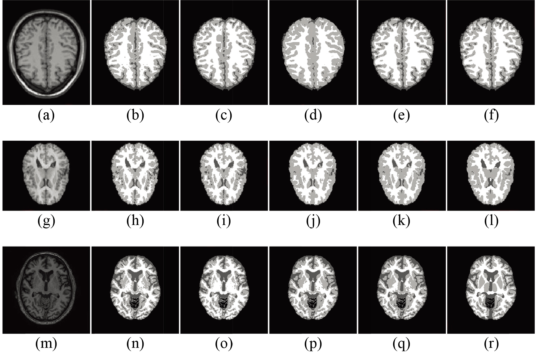
Figure 1 shows the example slices with respect to MR scan and ground truth. For BrainWeb subset, 4 compared methods revealed similar results referred to the ground truth. The presented work obtained minor advantage: no isolated tissue label was found by Method A due to imaging noises; Method B and C both detected less CSF than the proposed one when facing with intensity bias field. In IBSR comparison, tissue bias field again increased classification difficulty. Visually, Method A and B failed to precisely distinguish CSF from GM. The proposed method apparently outperformed Method C with better results, especially at the putamina and thalami. For MRBrainS13, Method B could not identify putamen and globus pallidus GM. Method A and C had improved performance but suffered from considerable label noise or thalami GM mis-labeling.

The first GMM iteration of the proposed pipeline is activated from a “simple” input generated by KMeans and tissue prior probability hypothesis, which is further detailed in Subsection 3.4 for final parameter initialization choice discussion. The pipeline is driven forward along the optimization path under global and local constraints. The spatial information employs a combination of posterior term for global constraint characterization and prior term for local characterization in Eq. (8). Definitely, an important balance should be carried out to combine both constraints for optimal classification in the meanwhile. Since both isolated tissue patches and biased boundaries by imaging defects result in label junction areas, indicating higher local label complexity in tissue neighborhood. Therefore, the voxel entropy in Eq. (6) is chosen as a ratio weighting after value normalization across the entire volume. The entropy guarantees the potential to approach classification optima gradually. The desired D⁢C measurements can be explained according to the nature of entropy for system complexity measuring. Before a voxel is relabeled, when obvious neighborhood tissue contrast occurs, the effect of posterior term gets enlarged to search for global information, and the prior term dominates under less label complexity, which means the internal part of brain tissues. Furthermore, the Euclidean distance weighting in Eq. (7) term also benefits non-isotropic MR scan segmentation accuracy.

3.4Experiment 2

The diversity of device vendors, scanning protocols, and imaging defects results in various intensity distributions and noise levels. This prevents GMM from maximizing its advantages when attempting to use one universal parameter initialization with high fitness. To evaluate independence on parameter choice, the pipelines were implemented 10 times with different KMeans centers and initial model prior probability in Eq. (2) by a pseudo-random function.

Figure 2.

Robustness performance under different parameter initialization choices.

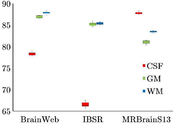
Tissue D⁢C inspected the accuracy under diverse conditions as Fig. 2. It can be seen that all mean tissue D⁢C measurements output tiny visible difference (less than 2.00), indicating a consistency against parameter choices.

Previous literature reported that multiple parameters in either KMeans or GMM led to entirely biased solution domains, and contrast significantly over arbitrary initializations [6]. Moreover, improper spatial information further trapped GMM by local optima in parameter estimation. On the contrary, the proposed method had distinct advantages in its robustness to initialization stage. That owes to the whole spatial information which focuses on performance improvement near tissue boundaries. The tissue label of each voxel cannot be simply determined unless the assembly weightings of its 26-neighbors are all taken into account. No matter how different parameter choices have been input, when label diversity is found, the entropy term will gradually find the solution that could lead to relatively consistent tissue boundaries. Only a few more iterations would take place to convergent results after continuous corrections.

For easy explanation, the eventual implementation set the KMeans centers as the 1/6, 3/6, and 5/6 fractional section of brain intensity range, and, arbitrary voxel tissue prior probability as 1/3. This was finally used in Experiment 1.

3.5Experiment 3

The execution time (in second) of tested methods is listed in Table 3. It is worth mentioning that the proposed method achieved the highest computation efficiency in this test compared with other GMM-based methods.

Originally, less attention had been paid to cope with the time cost, which commonly came from complicated calculation of the prior probability in Eq. (2). Authors tended to compromise to higher accuracy performance as the statement in [9]. Other techniques, such as parallel computing, might improve pipeline efficiency. In this work, the dedicated acceleration term in Eq. (12) enables a remarkably faster convergence of GMM iterations. It should be emphasized here that unlike additional items summed in log-likelihood in Eq. (9), this term is combined directly as weighting enhancement together with the E-step to obtain tissue posterior probability. That still contributes to a stable EM format, and does not bring in other burdens in parameter estimation procedures. Besides, the proposed entropy also decreases complex probability evaluation inside uniform label regions. The nature of entropy has more influence on the correction of mis-classified tissues.

To sum up, the proposed method yields more competitive performance. The key point is the entropy-enhanced spatial term to balance the ratio of prior and posterior probability. The posterior one dominates when various tissue label occurs in voxel neighborhood, and the prior one dominates in uniform labels. Hence, the effect of spatial information improves the resulting quality around tissue boundaries, where mis-classification is more likely to take place.

References

[1] | Lorio S, Lutti A, Kherif F, Ruef A, Dukart J, Chowdhury R, Frackowiak RS, Ashburner J, Helms G, Weiskopf N, Draganski B. Disentangling in vivo the effects of iron content and atrophy on the ageing human brain. Neuroimage. (2014) ; 103: : 280-9. |
[2] | Varnum MM, Ikezu T. The classification of microglial activation phenotypes on neurodegeneration and regeneration in Alzheimer’s disease brain. Archivum Immunologiae et Therapiae Experimentalis. (2012) ; 60: (4): 251-66. |
[3] | Zhao M, Lin HY, Yang CH, Hsu CY, Pan JS, Lin MJ. Automatic threshold level set model applied on MRI image segmentation of brain tissue. Applied Mathematics & Information Sciences. (2015) ; 9: (4): 1971-80. |
[4] | Cremers D, Rousson M, Deriche R. A review of statistical approaches to level set segmentation: Integrating color, texture, motion and shape. International journal of computer vision. (2007) ; 72: (2): 195-215. |
[5] | Guo Y, Liu Y, Oerlemans A, Lao S, Wu S, Lew MS. Deep learning for visual understanding: A review. Neurocomputing. (2016) ; 187: : 27-48. |
[6] | Balafar MA, Ramli AR, Saripan MI, Mashohor S. Review of brain MRI image segmentation methods. Artificial Intelligence Review. (2010) ; 33: (3): 261-74. |
[7] | Guerrout EH, Ait-Aoudia S, Michelucci D, Mahiou R. Hidden Markov random field model and Broyden-Fletcher-Goldfarb-Shanno algorithm for brain image segmentation. Journal of Experimental & Theoretical Artificial Intelligence. (2018) ; 30: (3): 415-27. |
[8] | Azimbagirad M, Simozo FH, Senra Filho AC, Junior LO. Tsallis-entropy segmentation through MRF and Alzheimer anatomic reference for brain magnetic resonance parcellation. Magnetic Resonance Imaging. (2020) ; 65: : 136-45. |
[9] | Ji Z, Huang Y, Xia Y, Zheng Y. A robust modified Gaussian mixture model with rough set for image segmentation. Neurocomputing. (2017) ; 266: : 550-65. |
[10] | Rosen KH, Krithivasan K. Discrete mathematics and its applications: with combinatorics and graph theory: Tata McGraw-Hill Education; (2012) . |
[11] | Gauvain JL, Lee CH. Maximum a posteriori estimation for multivariate Gaussian mixture observations of Markov chains. IEEE Transactions on Speech and Audio Processing. (1994) ; 2: (2): 291-8. |
[12] | Zhang Y, Brady M, Smith S. Segmentation of brain MR images through a hidden Markov random field model and the expectation maximization algorithm. IEEE Trans on Medcal Imaging. (2001) ; 20: : 45-57. |
[13] | Shannon CE. A note on the concept of entropy. Bell System Technical Journal. (1948) ; 27: (3): 379-423. |
[14] | Krishna K, Murty MN. Genetic K-means algorithm. IEEE Transactions on Systems, Man, and Cybernetics, Part B (Cybernetics). (1999) ; 29: (3): 433-9. |
[15] | Dempster AP, Laird NM, Rubin DB. Maximum likelihood from incomplete data via the EM algorithm. Journal of the Royal Statistical Society: Series B (Methodological). (1977) ; 39: (1): 1-22. |
[16] | BrainWeb, http://brainweb.bic.mni.mcgill.ca/brainweb. |
[17] | IBSR: Tool/Resource Info – NITRC, https://www.nitrc.org/projects/ibsr. |
[18] | The MRBrainS13 Workshop, https://mrbrains13.isi.uu.nl/. |
[19] | Dice LR. Measures of the amount of ecologic association between species. Ecology. (1945) ; 26: (3): 297-302. |