
Gastrointestinal stromal tumors diagnosis on multi-center endoscopic ultrasound images using multi-scale image normalization and transfer learning
Abstract
BACKGROUND:
Automated diagnosis of gastrointestinal stromal tumors’ (GISTs) cancerization is an effective way to improve the clinical diagnostic accuracy and reduce possible risks of biopsy. Although deep convolutional neural networks (DCNNs) have proven to be very effective in many image classification problems, there is still a lack of studies on endoscopic ultrasound (EUS) images of GISTs. It remains a substantial challenge mainly due to the data distribution bias of multi-center images, the significant inter-class similarity and intra-class variation, and the insufficiency of training data.
OBJECTIVE:
The study aims to classify GISTs into higher-risk and lower-risk categories.
METHODS:
Firstly, a novel multi-scale image normalization block is designed to perform same-size and same-resolution resizing on the input data in a parallel manner. A dilated mask is used to obtain a more accurate interested region. Then, we construct a multi-way feature extraction and fusion block to extract distinguishable features. A ResNet-50 model built based on transfer learning is utilized as a powerful feature extractor for tumors’ textural features. The tumor size features and the patient demographic features are also extracted respectively. Finally, a robust XGBoost classifier is trained on all features.
RESULTS:
Experimental results show that our proposed method achieves the AUC score of 0.844, which is superior to the clinical diagnosis performance.
CONCLUSIONS:
Therefore, the results have provided a solid baseline to encourage further researches in this field.
1.Introduction
Gastrointestinal stromal tumors (GISTs) are the most common mesenchymal neoplasms with potential malignancy in the gastrointestinal tract [1]. According to the Fletcher’s criteria, they can be divided into four categories: the very low risk group, the low risk group, the moderate risk group and the high risk group [2]. As the risk level grows, tumor’s recurrence, metastasis and death increase. The surgical resection is regarded as the main treatment for GISTs [3]. The assessment of the preoperative malignancy risk plays a pivotal role on determining whether the patient need to receive the preoperative targeted therapy [4].
GISTs are clinically diagnosed mainly by two methods: the endoscopic ultrasound (EUS) screening and the biopsy pathology analysis [5, 6, 7]. EUS images are extremely sensitive to noises leading to serious artifact interference which may sometimes adversely affect the accuracy of the clinical diagnosis. It is extremely demanding to read EUS scans for radiologists and the diagnosis process is prone to the operator bias. The biopsy pathology is the gold standard for the risk level assessment of GISTs. However, the biopsy process takes the risk of causing tumor rupture and cancer spread as GISTs are often fragile [8]. Hence, it is meaningful to develop automated GISTs classification methods using EUS images so as to reduce the risks of biopsy.
In recent years, a great variety of deep learning based medical image classification methods have been proposed [9, 10]. Deep convolutional neural networks (DCNNs) have been demonstrated the remarkable ability in selecting distinctive features from medical images [11], thus to avoid the complicated feature extraction of traditional radiomics methods. The training process of DCNNs typically requires a large volume of training data. Nevertheless, the size of medical image dataset is often limited as medical data is either hard to collect or annotate. The proposal of transfer learning provides a new solution to this problem for the reason that shallow-layer features of deep neural networks are shared among images [12].
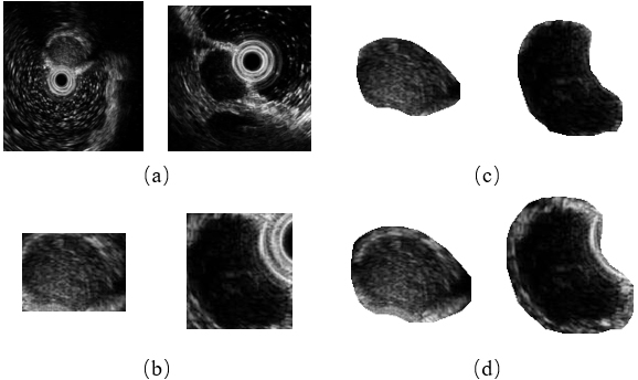
Figure 1.
Example images of four GISTs categories. (a) The very low risk, (b) the low risk, (c) the moderate risk, and (d) the high risk. The red line indicates tumor contours.
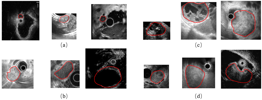
While extensive deep learning based studies focus on various kinds of medical image classification tasks, such as skin lesion classification, benign-malignant lung nodule identification and Alzheimer’s disease diagnosis, there is still a lack of researches on EUS images of GISTs. There are three main causes. First, these images are gathered by different scanners and vary in the size and spatial resolution, which makes a great data bias. It limits the performance of DCNNs to learn useful feature representations. Second, GISTs’ EUS images of four different risk levels have great intra-class variation and inter-class similarity. Three GISTs of each category are provided as examples in Fig. 1. As illustrated, these images have different sizes and spatial resolution. Some contain a circle representing the ultrasonic probe in the image while others do not. Moreover, we can see subtle differences among four groups but big visual differences among three cases of each group. It is extremely difficult to classify them without the expertise. Third, the maximum diameter of GISTs can range from millimeters to centimeters, thus posing a major challenge for extracting the size information and other textural, morphological features simultaneously in one DCNN framework because their majority always require a uniform input image size.
To tackle these problems, an integrated framework is proposed in this paper to classify higher-risk and lower-risk GISTs in multi-center dataset using multi-scale image normalization and transfer learning. The framework consists of three parts: a multi-scale image normalization block, a multi-way feature extraction and fusion block, and a classifier. EUS images are first normalized to the same size and same resolution, respectively. In order to keep tumors’ edge information and remove the background interference as well, we extract regions of interest (ROIs) using dilated tumor segmentation masks. Then, tumors’ textural and morphological features are extracted from same-size images using a transfer learning based CNN model while the size information is calculated from same-resolution images individually. We also include two demographic factors (age and sex) in our multi-way feature extraction and fusion block. Finally, an XGBoost classifier is established to predict the tumor’s risk level using all features.
To the best of our knowledge, this work is one of the first to apply deep learning methods to GISTs classification tasks on multi-center EUS images. Our main contributions are summarized as follows:
1) To solve the problem of multi-center data bias, we propose an effective multi-scale image normalization method by resizing EUS images to the same size and same resolution separately preparing for following feature extraction.
2) Considering that GISTs are visually similar among different risk groups, we design a multi-way feature extraction and fusion module to obtain more distinguishing features. Then, we fuse deep features extracted from a CNN model with size features of tumors and demographic information (age and sex) of patients to obtain a more complete feature representation.
3) To address the problem of limited data, transfer learning are used to prevent overfitting on small training datasets.
2.Method
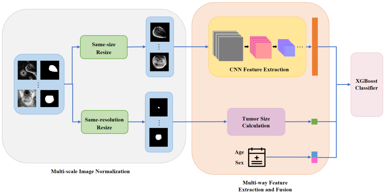
Our model consists of three parts: the multi-scale image normalization, the multi-way feature extraction and fusion, and classification. In the first place, the original endoscopic ultrasound scans together with the segmentation masks of tumors are normalized to the same size and same resolution in parallel. After preprocessing, a CNN model is built to extract tumors’ textural and morphological features from same-size images while tumors’ size information is obtained from same-resolution segmentation masks. The demographic information (age and sex) is also encoded as clinical features. Finally, an XGBoost classifier is established based on merged features. A schematic diagram of our framework is illustrated in Fig. 2. We now go into more details of this framework.
Figure 2.
The architecture for the proposed framework.
2.1Multi-scale image normalization
As mentioned above, EUS images from different centers vary greatly in the size and spatial resolution. As a result, tumors with similar physical sizes may look completely different in the image. Therefore, the image normalization is indispensable.
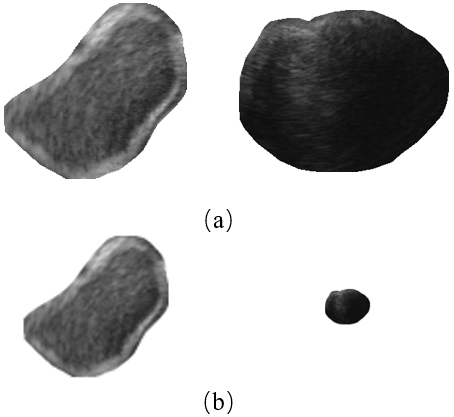
Traditional normalization methods simply resize all images to the same resolution. Nevertheless, it is not a good choice for GISTs. Because big tumors can be several times larger than those small ones, small tumors will be shrunk to only few pixels after resizing. Examples are given in Fig. 3. As shown in Fig. 3, the texture of the small tumor (the right column) can be observed clearly before resizing, while after resizing, a majority part of detailed information was lost.
Figure 3.
An illustration of severe information lost for small tumors after resizing all images to the same spatial resolution. (a) Before resizing and (b) after resizing.
Hence, in order to consider GISTs’ size information and textural information at the same time, we design a multi-scale image normalization module with two branches executing in parallel. A detailed architecture of this module is given in Fig. 4.
Figure 4.
The architecture of our proposed multi-scale image normalization module.
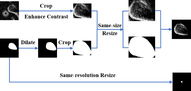
In one branch, we first extract a ROI in the original image to ensure inputs of the feature extraction module are tumor areas. Rather than using the corresponding segmentation mask, we dilate the mask and crop the original image according to the minimum bounding rectangle box of the dilated mask. In this way, the edge information of tumors can be reserved. This is important because GISTs with obscure boundaries tend to have the higher relevance with potential malignancy while lower-risk tumors have more smooth boundaries. After a contrast enhancing step, a same-size resizing operation is performed on all ROIs while keeping the aspect ratio unchanged. To reduce the possible background interference, we multiply the ROI and the dilated mask to remove background areas. Finally, the ROI is placed on the center of a black background with a size of 224
In another branch, a same-resolution resizing operation is performed on all original segmentation masks. After resizing, size differences among tumors can be obviously observed. Then, size features can be extracted in the feature extraction block individually.
2.2Multi-way feature extraction and fusion
In this section, we extract tumors’ textural and morphological features using the CNN as a deep feature extractor. Besides, the size features of tumors and the demographic features of patients are also encoded, respectively. These three kinds of features are then fused to acquire final features.
2.2.1CNN feature extraction
Due to a limited training dataset, simply training a CNN model from scratch may result in two problems. On the one hand, deep neural networks are prone to overfitting when only a small dataset is given. On the other hand, it is comparatively hard for neural networks to learn distinguishing features without enough data. Hence, we decide to strengthen the feature extraction ability of the CNN via transfer learning.
Transfer learning can be recognized as reusing a pre-trained model on a new target task. In the field of computer vision, early layers of neural networks are usually responsible for detecting edges and shapes These general low-level features are shared among all images. For example, the shape and contour of tumors are very similar to some objects in natural images. Therefore, we can take advantage of pre-trained weights on big natural image datasets as the starting point for a new task and then refine the model using data available for the new task.
To utilize the extraordinary feature extraction ability of models learned on large image datasets for characterizing GISTs, we choose a ResNet-50 [13] model pre-trained on the ImageNet dataset as the transfer learning backbone. We replace the original last fully connected layer (designed for 1000 classes) by a new one with only two neurons. To achieve fast adaptation to the GIST classification task, the whole model is fine-tuned with a different learning rate on the new classification layer and other layers. The output of the second last layer (the input of the last fully connected layer) is defined as a 2048-dimensional deep feature.
The extracted ROIs after same-size resizing are used as inputs of the CNN model. Due to the relatively small training set, the data augmentation is adopted to add variants in the CNN training phase to further alleviate the overfitting of deep learning models. After the training, the best performed model on the validation set is selected as the feature extractor. CNN features of all images in the dataset are then extracted and saved without any augmentation.
The traditional cross-entropy loss with class weighting strategy is applied in our model’s training. Each class is multiplied by a factor
(1)
where
The standard cross-entropy loss can be defined as:
(2)
where
After multiplying by the weighting term, the loss can be expressed as:
(3)
2.2.2Tumor size calculation
Tumors’ segmentation masks with the same resolution are used to calculate their relative sizes. The area of masks after scaling to (0, 1) can be regarded as tumor size feature representations.
2.2.3Demographic features
Two demographic features, age and sex, of each patient are also included in our study. To encode the data as feature vectors, the ages are represented by normalized continuous numerical values while the sex information is represented by discrete values of one (for male) and zero (for female).
2.3Classification model
The eXtreme Gradient Boosting (XGBoost [14]) algorithm is used in this study to establish a classifier at the top of our entire framework. XGBoost is an integrated learning algorithm built on the Gradient Boosting (GB) to achieve the high classification performance through the iterative computation of weak classifiers. Here, the input of the XGBoost classifier is a 2051-dimensional feature vector and the output is the probability that a tumor belongs to the higher-risk group. Detailed information of the feature vector size is given in Table 1.
Table 1
Detailed information of the feature vector size
| Feature name | CNN feature | Tumor size feature | Demographic feature |
|---|---|---|---|
| Feature size | 2048 | 1 | 2 |
Considering that more than one image may be available for one patient, the risk level prediction results are finally decided on all images’ diagnostic results of a certain patient using a majority voting algorithm.
3.Experiments
3.1Dataset
The endoscopic ultrasound images of 914 patients (1824 images) were collected from 18 hospitals in China. Five ultrasound units, Fuji SU9000, Fuji SU8000, Olympus Alpha 10, Olympus EU-ME1 and Olympus eu-ME2 were used. All subjects had signed the written informed consent for EUS imaging and data to be donated for scientific research. The demographic and clinical information of all studied patients are depicted in Table 2. All images were segmented manually by experienced doctors.
Table 2
The clinical and demographic information of patients in the dataset. (Values are reported as mean
| Number of patients | Number of images | Age (years) | Gender (male/female) | |
|---|---|---|---|---|
| Very low | 420 | 870 | 57.27 | 147/273 |
| Low | 326 | 643 | 58.33 | 145/181 |
| Moderate | 114 | 219 | 59.19 | 52/62 |
| High | 54 | 92 | 56.48 | 33/21 |
Four types of GISTs are all covered in this datasheet. The very low risk level and the low risk level were divided into the lower-risk group (LRG) while the moderate risk level and the high risk level were merged as the higher-risk group (HRG). Positive samples (HRG) are five times smaller than negative samples (LRG). Because all images were obtained in different times and locations with different devices, there exists a huge difference on the data distribution. Original sizes of all images range from 100 to 1000 pixels around while their spatial resolution differ from 17 to 286 pixels representing one certain centimeter.
In this study, 679 patients (1390 images in total) were randomly chosen as the training set. A validation set containing 54 patients with only one image provided for each individual was built so as to choose the model with the best performance on one single image. Rest patients were separated as the individual testing set. The detailed information of data partition is shown in Table 3.
Table 3
The details of dataset distribution
| The LRG | The HRG | ||||
|---|---|---|---|---|---|
| Very low | Low | Moderate | High | ||
| Training | Number of patients | 319 | 248 | 74 | 38 |
| Number of images | 675 | 495 | 152 | 68 | |
| Validation | Number of patients | 17 | 13 | 18 | 6 |
| Number of images | 17 | 13 | 18 | 6 | |
| Testing | Number of patients | 84 | 65 | 22 | 10 |
| Number of images | 178 | 135 | 49 | 18 | |
3.2Evaluation metrics
Four evaluation metrics were involved to quantitatively evaluate the model performance: the accuracy (ACC), the area under the receiver operator curve (AUC), the sensitivity (SENS) and the specificity (SPEC). The ACC delivers the model’s overall ability in classifying tumors’ risk levels while the SENS and the SPEC metrics measure the model’s ability to classify higher-risk samples and lower-risk ones, respectively. The AUC represents the probability that a classifier grades a randomly selected positive sample higher than a negative one. The detailed definitions are as follows:
(4)
(5)
(6)
(7)
where
3.3Experimental settings
Here we elaborate implementation details of our proposed method first and then introduce comparison experiments.
3.3.1Implementation details
In the CNN training stage, several kinds of data augmentation strategies were utilized, including the random crop, the random horizontal or vertical flip and the random rotation. To ensure the completeness of tumor regions, zero padding was implemented before random cropping. An Adam optimizer was used and the initial learning rate of the classification layer was set to 0.00005 while that of other layers was set to one-tenth of it. The learning rate was reduced by half every 10 epochs. The batch size was set to 64. The maximal fine-tuning epochs was 50.
In the XGBoost classifier, a learning rate of 0.05, a maximum tree depth value of 4 and a maximum iteration step of 200 were used.
3.3.2Comparison experiments
In order to prove the superiority of the proposed method, several comparison experiments are designed.
To demonstrate the necessity of the multi-scale image normalization module, two comparison experiments were conducted. Firstly, instead of doing the normalization process, we simply cropped a patch from the original image using the minimum bounding rectangle of the corresponding segmentation mask. The cropped patch was padded to a square before resizing to 224
To validate the effectiveness of the multi-way feature extraction and fusion module, we compared the classification performance among three different kinds of input features: only CNN features, CNN features plus the size feature and CNN features plus the size feature and demographic features (our proposed method).
To evaluate the effectiveness of transfer learning, we trained a ResNet-50 from scratch as the CNN feature extractor for the comparison. The initial learning rate was set to 0.001 and halved every 15 epochs. The maximum training epoch number was set to 100. Considering that in addition to the ResNet-50, the ResNet-18 [13], the VGGNet-16 [15], the MobileNetV2 [16], the DenseNet-121 [17], the AlexNet [18] and the Inception-v3 [19] are also six of most frequently-used DCNN models, we also evaluated the model performance when using different DCNNs as transfer backbones.
Implementation details of comparison experiments maintained same as the proposed method unless otherwise specified.
4.Results and discussion
In this section, we first present and analyze the results of our proposed method and comparison experiments. Then, limitations of our method are discussed.
4.1Impact of multi-scale image normalization
In our proposed method, we design a multi-scale image normalization module for multi-center data. To demonstrate that the designed block is effective, we did two comparison experiments as mentioned in 3.3.2. Results are depicted in Table 4.
Table 4
Comparison results of different normalization methods
| Method | ACC | AUC | SENS | SPEC |
|---|---|---|---|---|
| Without normalization | 0.774 | 0.8 | 0.563 | 0.819 |
| Normalization using original masks | 0.768 | 0.829 | 0.75 | 0.772 |
| Normalization using dilated masks (the proposed method) | 0.796 | 0.844 | 0.813 | 0.792 |
As reported in Table 4, our method with a multi-scale image normalization module outperforms other two methods. The method without the normalization reports an extremely low SENS indicating that the model is unable to classify higher-risk GISTs. While after the multi-scale image normalization, the SENS score has witnessed an increase from 0.563 to 0.75 (with original masks) and 0.813 (with dilated masks). This is mainly because the size information and textural information of GISTs are considered simultaneously.
Meanwhile, the further consideration on the edge information of GISTs also improves the model performance on all four metrics. Two examples of different ROI extraction methods are given in Fig. 5. As depicted in Fig. 5 directly cropping a patch using the original mask (Fig. 5b) may bring the background interference when tumors are close to the ultrasonic probe (the right column). Although this problem can be solved by multiplying the cropped patch with the mask (Fig. 5c), the tumors’ edge information is discarded at the same time. Therefore, we use a dilated mask to keep the edge information while reducing the possible interference as well.
Figure 5.
The comparison of different ROI extraction methods. (a) Original image, (b) cropping a patch using the original mask, (c) cropping a patch using the original mask and multiplying with it, and (d) cropping a patch using the dilated mask and multiplying with it (our proposed method).
4.2Impact of multi-way feature extraction and fusion
A multi-way feature extraction and fusion block is used in this study to extract CNN features, size and demographic features separately. To prove the advantages of jointly using three kinds of features, we designed two comparison experiments as stated in 3.3.2. Table 5 lists quantitative results while Fig. 6 plots the corresponding receiver operator curve (ROC).
Table 5
Comparison results of methods using different features as classifier’s inputs
| Method | ACC | AUC | SENS | SPEC |
|---|---|---|---|---|
| CNN features only | 0.768 | 0.775 | 0.719 | 0.779 |
| CNN features | 0.779 | 0.838 | 0.781 | 0.779 |
| CNN features | 0.796 | 0.844 | 0.813 | 0.792 |
Figure 6.
ROC curves of methods using different features as classifier’s inputs.
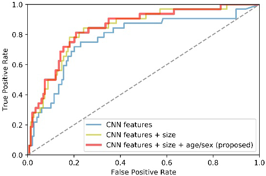
From Table 5 and Fig. 6, we can observe that both size and demographic information facilitate our model performance. To be specific, the AUC and SENS scores got a considerable improvement of about 6% when the size information is added. Furthermore, the proposed method generally outperforms the method that does not consider demographic factors of patients. It suggests that the demographic information is helpful to facilitate the classification performance. In a word, the multi-way feature extraction and fusion block has the superior ability to obtain a more complete feature representation.
4.3Impact of transfer learning
To prove that transfer learning with ResNet-50 can boost the performance of GISTs classification when limited data is available, the performance of our proposed method based on a pre-trained ResNet-50 was compared with a ResNet-50 trained from scratch. We also tested the performance when using different transfer learning backbones. Quantitative results are given in Table 6.
Table 6
Comparison results of different transfer learning strategies
| Method | Backbone model | ACC | AUC | SENS | SPEC |
|---|---|---|---|---|---|
| Train from scratch | ResNet-50 | 0.746 | 0.835 | 0.719 | 0.752 |
| Transfer learning | VGGNet-16 | 0.768 | 0.840 | 0.781 | 0.765 |
| MobileNetV2 | 0.757 | 0.835 | 0.750 | 0.758 | |
| DenseNet-121 | 0.774 | 0.845 | 0.750 | 0.779 | |
| AlexNet | 0.762 | 0.828 | 0.75 | 0.765 | |
| Inception-v3 | 0.780 | 0.836 | 0.750 | 0.785 | |
| ResNet-18 | 0.774 | 0.854 | 0.813 | 0.765 | |
| ResNet-50 (proposed) | 0.796 | 0.844 | 0.813 | 0.792 |
As reported in Table 6, the performance of transfer learning strategies is much better than training from scratch in general. Transferring image representation abilities of pre-trained models on large datasets helps to characterize GISTs and obtain a better feature representation.
When comparing the classification performance among different pre-trained models, the ResNet-50 and ResNet-18 produce best results. This can be credited with residual blocks in ResNet architectures to capture distinguishing features of input images during the deep backpropagation. As illustrated in Table 6, although the ResNet-18 reports a slightly higher AUC value, the ResNet-50 achieves more balanced results, especially for the SENS and SPEC, so we finally choose the ResNet-50 as the backbone.
4.4Robustness of the proposed method
To address the selection bias of the limited data, repeated random dataset partition was applied to evaluate the performance stability and reliability of our proposed method. The process of splitting the dataset was repeated for another 5 times. The mean and standard deviation of the experimental results are reported in Table 7. As listed in Table 7, the performance of our model is stable with relatively low standard deviation on all four metrics. Hence, the robustness of the proposed method under different dataset partition scenarios can be well demonstrated.
Table 7
The mean and standard deviation of the experimental results
| ACC | AUC | SENS | SPEC | |
|---|---|---|---|---|
| Mean | 0.809 | 0.851 | 0.806 | 0.809 |
| Standard deviation | 0.006 | 0.010 | 0.026 | 0.010 |
4.5Comparison with traditional radiomics methods
Besides deep learning based methods, radiomics is another kind of common methodologies in the medical image classification field. Li et al. [20] designed a traditional radiomics method for GIST classification task. Despite of the similar model performance the radiomics method relies heavily on hand-crafted features which is much less effective. What’s more, the specificity of radiomics features is not studied for a specific disease. Thus, the stability of the predictions is prone to suffer from dataset selection bias. However, deep learning based methods can automatically extract distinguishable features of GISTs. Once the model training process is finished, the feature extraction is expected to be fast and accurate.
4.6Limitations and future work
Although we have obtained good results, there are still several limitations to be considered in this study. First, the unbalanced dataset brings a big challenge on the classification task. We will make efforts to establish a more complete and balanced database in the future. Second, the existing framework utilizes a CNN model whose weights are transferred from the ImageNet dataset. However, domain differences between natural images and medical ones may limit the model performance. Studying more effective transfer learning methods will be included in our later work.
5.Conclusion
We propose a multi-scale image normalization and transfer learning based framework for HRG-LRG GIST classification on multi-center endoscopic ultrasound images. The proposed framework can automatically extract discriminative features from multi-center data without requiring any expert knowledge for defining features. Especially, it can explicitly incorporate the size information of tumors and demographic information (age and sex) of patients into the predicting process. Results demonstrate that our model succeed in distinguishing 32 case HRG tumors from 149 LRG tumors with achieving an ACC of 0.796, an AUC of 0.844, a SENS of 0.813, and a SPEC of 0.792, which could provide a favorable reference for the clinical diagnosis.
Acknowledgments
This work was supported by the National Natural Science Foundation of China (Grants 61771143, 61871135 and 81830058) and the Science and Technology Commission of Shanghai Municipality (Grants 18511102904 and 17411953400).
Conflict of interest
None to report.
References
[1] | Joensuu H, Hohenberger P, Corless CL. Gastrointestinal stromal tumour. The Lancet. (2013) ; 382: (9896): 973-983. |
[2] | Agaimy A. Gastrointestinal stromal tumors (GIST) from risk stratification systems to the new TNM proposal: More questions than answers? A review emphasizing the need for a standardized GIST reporting. Int J Clin Exp Pathol. (2010) ; 3: (5): 461-471. |
[3] | Yang Z, Gao Y, Fan X, et al. A multivariate prediction model for high malignancy potential gastric GI stromal tumors before endoscopic resection. Gastrointest Endosc. (2020) ; 91: (4): 813-822. |
[4] | Rammohan A, Sathyanesan J, Rajendran K, Pitchaimuthu A, Perumal SK, Srinivasan U, et al. A gist of gastrointestinal stromal tumors: A review. World. J. Gastrointest. Oncol. (2013) ; 5: (6): 102-112. |
[5] | Chak A, Canto MI, Rösch T, Dittler HJ, Hawes RH, Tio TL, et al. Endosonographic differentiation of benign and malignant stromal cell tumors. Gastrointest. Endosc. (1997) ; 45: : 468-473. |
[6] | Casali PG, Blay JY. Gastrointestinal stromal tumors: ESMO clinical practice guidelines for diagnosis, treatment and follow-up. Ann. Oncol. (2010) ; 21: : 98-102. |
[7] | Faulx AL, Kothari S, Acosta RD, Agrawal D, Bruining DH, Chandrasekhara V, et al. The role of endoscopy in subepithelial lesions of the GI tract. Gastrointest Endosc. (2017) ; 85: (6): 1117-1132. |
[8] | Blackstein M, Blay J-Y, Corless C, Driman D, Riddell R, Soulieres D, et al. Gastrointestinal stromal tumours: consensus statement on diagnosis and treatment. Can. J. Gastroenterol. (2006) ; 20: (3): 157-163. |
[9] | Anthimopoulos M, Christodoulidis S, Ebner L, Christe A, Mougiakakou S. Lung pattern classification for interstitial lung diseases using a deep convolutional neural network. IEEE Trans Med Imaging. (2016) ; 35: (5): 1207-1216. |
[10] | Yu L, Chen H, Dou Q, Qin J, Heng P. Automated melanoma recognition in dermoscopy images via very deep residual networks. IEEE Trans Med Imaging. (2017) ; 36: (4): 994-1004. |
[11] | Xie Y, Xia Y, Zhang J, Song Y, Feng D, Fulham M, et al. Knowledge-based collaborative deep learning for benign-malignant lung nodule classification on chest CT. IEEE Trans. Med. Imaging. (2019) ; 38: : 991-1004. |
[12] | Shin HC, Roth HR, Gao M, Lu L, Xu Z, Nogues I, et al. Deep convolutional neural networks for computer-aided detection: CNN architectures, dataset characteristics and transfer learning. IEEE. Trans. Med. Imaging. (2016) ; 35: (5): 1285-1298. |
[13] | He K, Zhang X, Ren S, Jian S. Deep residual learning for image recognition. In: Proceedings of the IEEE Conference on Computer Vision and Pattern Recognition. (2016) June 26–July 1. Las Vegas, Nevada. |
[14] | Chen T, Guestrin C. XGBoost: a scalable tree boosting system. In: Proceedings of the 22nd ACM SIGKDD International Conference. (2016) August 24–27. San Francisco, United States. |
[15] | Simonyan K, Zisserman A. Very deep convolutional networks for large-scale image recognition. In: Proceedings of the International Conference on Learning Representations. (2015) May 7–9. San Diego, CA. |
[16] | Sandler M, Howard A, Zhu M, Zhmoginov A, Chen LC. MobileNetV2: inverted residuals and linear bottlenecks. In: Proceedings of the IEEE Conference on Computer Vision and Pattern Recognition. (2018) June 18–22. Salt Lake City, Utah. |
[17] | Huang G, Liu Z, Weinberger K. Densely connected convolutional networks. In: Proceedings of the IEEE Conference on Computer Vision and Pattern Recognition. (2017) July 21–26. Honolulu, Hawaii. |
[18] | Krizhevsky A, Sutskever I, Hinton GE. Imagenet classification with deep convolutional neural networks. In: Proceedings of the 25th International Conference on Neural Information Processing Systems. (2012) December 3–6. Lake Tahoe, Nevada. |
[19] | Szegedy C, Vanhoucke V, Loffe S, Shlens J Wojna Z. Rethinking the Inception architecture for computer vision. In: Proceedings of the IEEE Conference on Computer Vision and Pattern Recognition. (2015) June 8–10. Boston, Massachusetts. |
[20] | Li X, Jiang F, Guo Y, Jin Z, Wang Y. Computer-aided diagnosis of gastrointestinal stromal tumors: A radiomics method on endoscopic ultrasound image. Int. J. Comput. Assist. Radiol. Surg. 14: ((2019) ): 1635-1645. |


