
Computational analysis of aortic haemodynamics in the presence of ascending aortic aneurysm
Abstract
BACKGROUND:
The usefulness of numerical modelling of a patient’s cardiovascular system is growing in clinical treatment. Understanding blood flow mechanics can be crucial in identifying connections between haemodynamic factors and aortic wall pathologies.
OBJECTIVE:
This work investigates the haemodynamic parameters of an ascending aorta and ascending aortic aneurysm in humans.
METHODS:
Two aortic models were constructed from medical images using the SimVascular software. FEM blood flow modelling of cardiac cycle was performed using CFD and CMM-FSI at different vascular wall parameters.
RESULTS:
The results showed that highest blood velocity was 1.18 m/s in aorta with the aneurysm and 1.9 m/s in healthy aorta model. The largest displacements ware in the aorta with the aneurysm (0.73 mm). In the aorta with the aneurysm, time averaged WSS values throughout the artery range from 0 Pa to 1 Pa. In the healthy aorta, distribution of WSS values changes from 0.3 Pa to 0.6 Pa.
CONCLUSIONS:
In the case of an ascending aortic aneurysm, the maximum blood velocity was found to be 1.6 times lower than in the healthy aorta. The aneurysm-based model demonstrates a 45% greater wall displacement, while the oscillatory shear index decreased by 30% compared to healthy aortic results.
1.Introduction
According to the World Health Organization’s global statistics, one in three people dies from a cardiovascular disorder [1]. Moreover, the number of patients with a thoracic aortic aneurysm has increased in recent years. The aorta is the largest human artery [2], supplying oxygen-saturated blood to the entire body. Aortic aneurysms, which pose a high risk to human life, are among the most difficult vascular system pathologies to diagnose [3]. Aortic haemodynamics is an ongoing area of research aimed at determining the flow patterns and stresses occurring in the aorta. These parameters are used to detect and investigate the presence of cardiovascular diseases such as aortic aneurysms, dissections and atherosclerosis. However, the relationship between mechanical factors and haemodynamics may be difficult to monitor and quantify due to the many existing conditions in real patient data. Therefore, scientists use methods that mimic blood flow and the mechanical properties of vessels to simulate the human cardiovascular system. These studies include 3D printed aortic model tests [4, 5], silicone model experiments [6, 7], ex-vivo mechanical tests [8, 9] and numerical modelling methods [10, 11, 12].
Computational fluid dynamics (CFD) [13] uses digital computers to create quantitative predictions of fluid flow phenomena based on the conservation laws (i.e. mass, pulse and energy sustainability laws) that govern fluid motion. Using CFD makes it possible to visualise blood flow models, pressure gradients, deformations and stress distributions caused by vascular disease [14]. Such illustrations provide highly relevant and important information in the process of treating aneurysms, planning surgery, predicting the development of pathology and assessing the risks associated with the disease. This methodology offers the advantage of making the study of the deformities of vascular tissues and blood flow possible without surgical intervention. The main goal of this study is to analyse and evaluate physiologically significant parameters while comparing the results of modelling a healthy aorta and an aorta with aneurysm haemodynamics using equal boundary conditions. The effect of blood flow on the distribution of aortic wall stresses will be useful for future studies to evaluate the effect of these types of distributions on the risk of aortic aneurysm rupture.
2.Materials and methods
SimVascular software was used in a series of steps to solve the problems of computational fluid dynamics. The stages included geometry acquisition, identification and description of boundary conditions, selection of calculation type and equipment, calculation, processing and displaying the obtained results [15].
2.1Image acquisition and segmentation
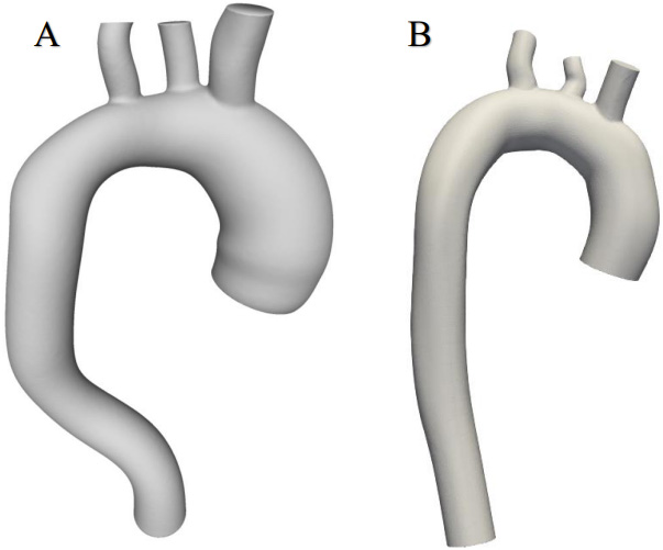
This work used CT thorax 3D imagery with an ascending aortic aneurysm [16] and the image of a healthy aorta from the SimTK database [17]. The SimVascular software package [18] was used to create a 3D aortic model using sections from medical images. The first step was to determine which parts of the medical image depicted the object of interest, which was achieved through volumetric image generation and threshold setting. Initially, the aortic centre points were postponed (Fig. 1), and the centre line of the flow beam was formed. Next, the left posterior artery, the left carotid artery, and the brachiocephalic artery were added to the baseline. The second step, as shown in Fig. 1, was the segmentation of the vessel, where the contour of the vessel was determined at the central points. In the process, 2D contours were generated at each point on the centreline. The contour was initiated by a dot and displayed in the directions of changing the intensity values to find the location of the most pronounced changes. After segmentation, the modelling tool was used to generate a 3D model of the aorta. At the sites of the aortic arch where the arterial bifurcations were present, surface smoothing and rounding of the arterial junctions were performed, and Meshmixer software was used to regenerate the model [19]. The SimVascular program was used to join all arterial walls into a single body. After model processing, 6 surfaces were obtained: 1 vessel wall and 5 caps (Fig. 2).
Figure 1.
Geometric model construction steps; flow waveform as an inlet boundary condition and RCR model as outlet boundary conditions.
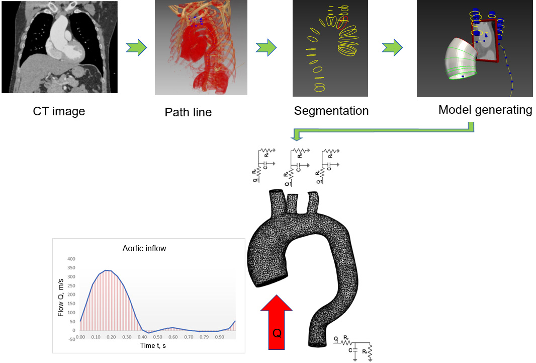
Figure 2.
Geometric models of aortas.
2.2Blood flow modelling
Blood flow was modelled using Navier-Stokes equations for Newtonian fluids. The storage of the mass and impulses of a non-compressed fluid in three dimensions can be expressed as follows:
(1)
where
Appropriate equations were needed to calculate blood viscosity in order to use this system of equations. The simplest model is Newtonian fluid, which has constant viscosity. Blood is described as an uncompressed Newtonian fluid, and flow is laminar. Dynamic blood viscosity
The inflow boundary conditions are the waveform of the fluid flow that simulates flow from the aortic valve. Because the flow of blood in the human body pulsates, a constant velocity at the inlet does not simulate the actual flow, which should be reported as a variable periodic profile in this case. Each cardiac cycle is a combination of a systolic phase and a diastolic phase. Therefore, this work used a temporal profile describing the flow during systole and diastole. Assuming a heart rate of 60 beats per minute, the duration of each cycle is 1 s; under these conditions, the blood flow
The Windkessel haemodynamic model [21], used to restore a patient’s aortic blood pressure, describes the heart and blood vessels as a closed hydraulic system. The Windkessel model is most used to describe load during the cardiac cycle. This approach links the pressure and blood flow in the aorta and describes the ability of the arteries to withstand deformities as the volume changes. In comparison, SimVascular uses resistance-capacitance-resistance (RCR) outlet conditions [22]. The downstream pressure is expressed through an ordinary differential equation similar to the relation between voltage and current in electric circuits. This type of boundary condition uses a reduced-sequence vascular model based on an analogue of the electrical circuit described above. According to this theory, vascular behaviour is represented by three parameters: proximal resistance
(2)
(3)
where
Determining the boundary conditions in the SimVascular program requires first calculating the total system resistance. This value can be found by dividing the mean pressure
(4)
where
By introducing the total resistance, SimVascular concretely calculates the proximal and distal resistance for each outlet using the outlets cups areas.
SimVascular uses the open-source TetGen meshing method [24]. In the aorta with an aneurysm (Fig. 3), an FE mesh of 146,262 elements was generated. In contrast, the healthy aorta model mesh consisted of 67,572 elements.
2.3Vessel wall parameters
The calculation was performed using different wall parameters. Rigid settings, meaning that the walls were rigid and non-slip, were used to examine blood velocities and pressure. The use of the rigid wall approximate condition reflected the fact that, under normal conditions, didn’t need to use deformable wall settings, because the displacement of the walls does not significantly change the velocity field. Obtaining the value of wall displacements as well as the wall shear stress (WSS) and oscillatory shear index (OSI) involved using the boundary conditions under which the aortic wall was modelled as a linear elastic material that could have had the same or variable modulus of elasticity and thickness along the vessel (Table 1). This approach entailed a simplified fluid-structure interaction (FSI) method using the coupled momentum method (CMM) [25]. This CMM-FSI formulation shows the traditional stabilized finite element formula for the Navier-Stokes equations in the rigid wall region and modifies it to account for the deformation of the fluid domain.
Table 1
Biomechanical aortic wall parameters
| Parameter | Value |
|---|---|
| Thickness | 1.8 mm |
| Elastic modulus | 4000000 Pa |
| Poisson ratio | 0.5 |
| Shear constant | 0.8333333 |
| Density | 1.0 |
| Pressure | 133300 Pa |
Figure 3.
Generated FE mesh.
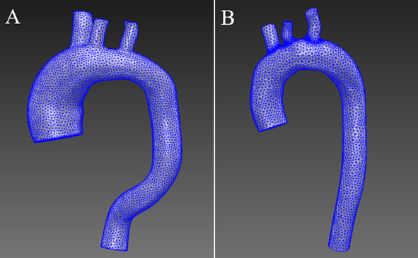
Figure 4.
Schematic illustration of wall shear stress of blood flow in the aorta.
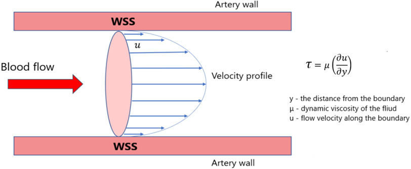
Figure 5.
Distribution of blood flow velocities in the aorta with aneurysm.
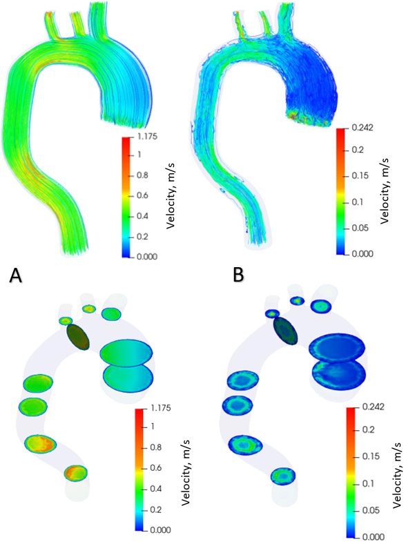
Figure 6.
Distribution of blood flow velocities in healthy aorta.
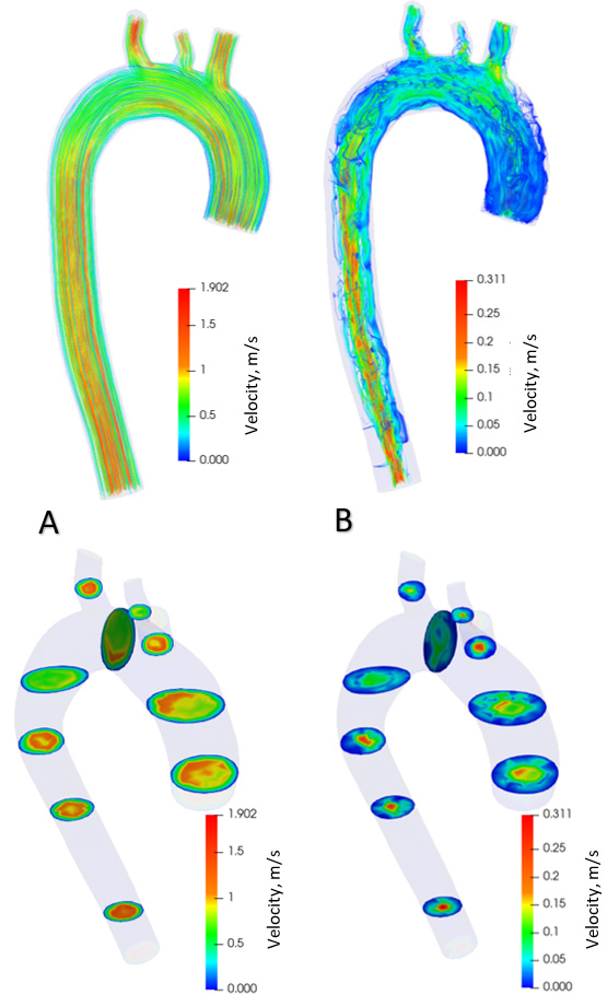
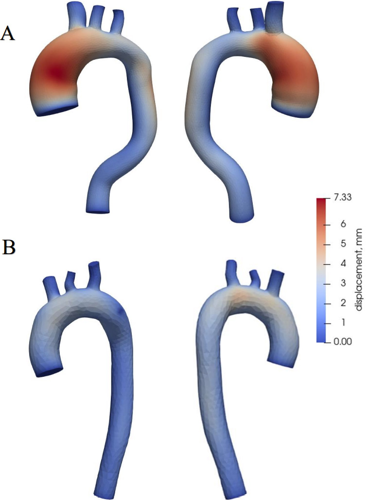
Figure 7.
Aortic wall displacements.
WSS and OSI were determined during the calculation. WSS a frictional force caused by blood flowing along the vessel wall (Fig. 4) and can alter the integrity and biomechanical strength of the intercellular matrix of the vessel wall. WSS expresses the force per unit area by which a wall acts on a liquid in the direction of a local tangent plane [26] as follows:
(5)
where
The fluctuating shear index is another significant haemodynamic parameter used to assess WSS because they are related. OSI is a dimensionless parameter used to identify WSS fluctuations from flow direction during the cardiac cycle [27]:
(6)
where WSS is the instantaneous vector of wall shear stresses,
OSI shows the physical deviation of the WSS vector from its predominant axial flow direction along the parallel vector [28].
2.4Simulation
Simulations were performed over 6 cardiac cycles to stabilise flow velocity and pressure fields. The number of time steps per cycle was 1,000 with a fixed time step size of 0.001 s. The simulation results were evaluated during the last cardiac cycle.
3.Results
The calculation results are presented graphically using the resulting images. Blood flow modelling was performed for a model with an aneurysm and a healthy aorta. Identical parameters and boundary conditions were used during the simulation. The open-source visualisation program ParaView [29] was used to visualise the results.
Figure 5 shows the distribution of blood flow in the aorta with aneurysm in the systolic phase (Fig. 5A) and diastolic phase (Fig. 5B) over one cardiac cycle. The contours of the flow velocity diagram are also shown. During the systole, the blood velocity varies from 0 to 1.18 m/s. In the diastole, the speed varies from 0 to 0.24 m/s. The maximum flow velocities in the systole are formed in the branching and descending part of the aorta. During diastole, the maximum flow rate is in the ascending aorta at the onset of the aneurysm. Figure 6 shows the distribution of blood flows in a healthy aorta, depicting the systole (Fig. 6A) and diastole (Fig. 6B) during one cardiac cycle. The contours of the velocity diagram are shown. During the systole, the blood velocity varies from 0 to 1.9 m/s. In the diastole, the speed varies from 0 to 0.31 m/s. The maximum flow rate values are formed in the branching and descending part of the aorta.
Aortic wall displacements are shown in Fig. 7. The largest displacements are in the aorta with the aneurysm (Fig. 7A), reaching 0.73 mm at the site of the ascending aorta, where the aneurysm is dilated. In a healthy aorta (Fig. 7B), the maximum value of displacements is 0.4 mm, and these displacements occur in the ascending aorta and the aortic arch.
Figure 8 shows pressure distribution during systole and diastole phases. Blood pressure is 120 mm Hg during systole (Fig. 8A) and 73 mm Hg during diastole in the aorta with aneurysm (Fig. 8B). The maximum pressure values in the systole are in the ascending aorta and aortic arch, and in the descending aorta in the diastole. During systole in a healthy aorta (Fig. 8C), the blood pressure is 122 mm Hg, in diastole (Fig. 8D) 75 mm Hg.
Figure 8.
Aortic pressure distribution during systole and diastole phases.
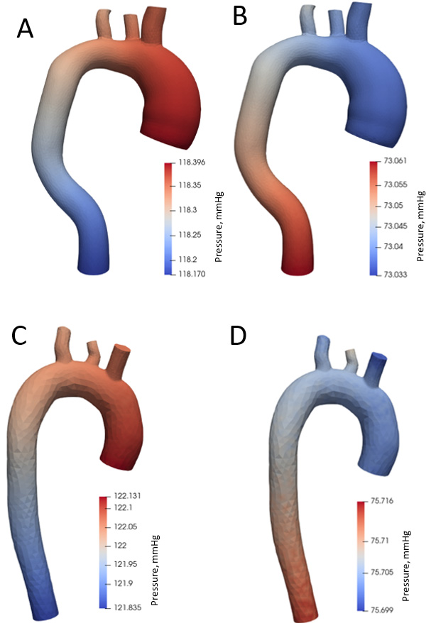
Figure 9.
Aortic wall shear stress distributing during systole and diastole phases.
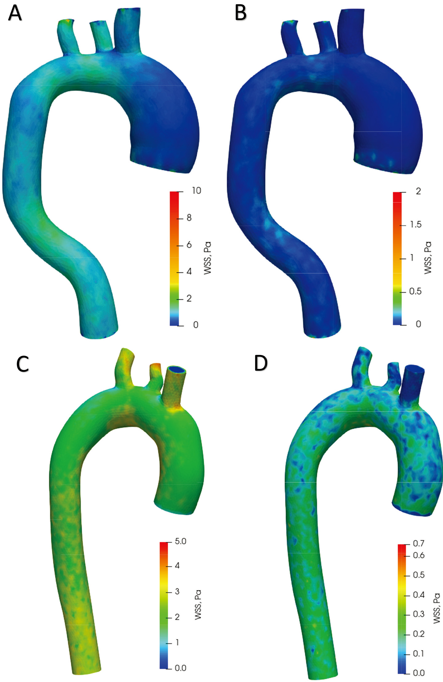
Figure 9A offers plots of WSS distribution diagrams in the aorta with aneurysm during systole. In the ascending aorta, the WSS values in the aortic arch range from 0 Pa to 2.5 Pa. In the descending aorta, the WSS is from 0.3 Pa to 3 Pa. A large WSS is formed at points on the branches of the aortic arch up to 10 Pa. The lowest WSS value is in the ascending aortic aneurysm. Figure 9B shows the distribution of WSS in the diastolic phase. In the whole aorta (except the aortic branches), the WSS ranges from 0 Pa to 0.5 Pa. The highest WSS value is in the aortic branches – up to 2 Pa. The values in the aortic branches are highly dependent on the geometry; thus, a high value may be due to the structure of the model. Figure 9C displays WSS distribution diagrams in a healthy aorta during systole. WSS values range from 1.5 Pa to 3.3 Pa in the ascending aorta, aortic arch and descending aorta. The highest stresses occur on the branches of the aortic arch up to 5 Pa. The distribution of WSS in the diastole phase is shown in Fig. 9D. In the whole aorta (except the aortic branches), the WSS ranges from 0 Pa to 0.4 Pa. The highest WSS value in the branches of the aortic arch is up to 0.7 Pa.
Figure 10.
Time average wall shear stress and oscillatory shear index distribution during one heart cycle.
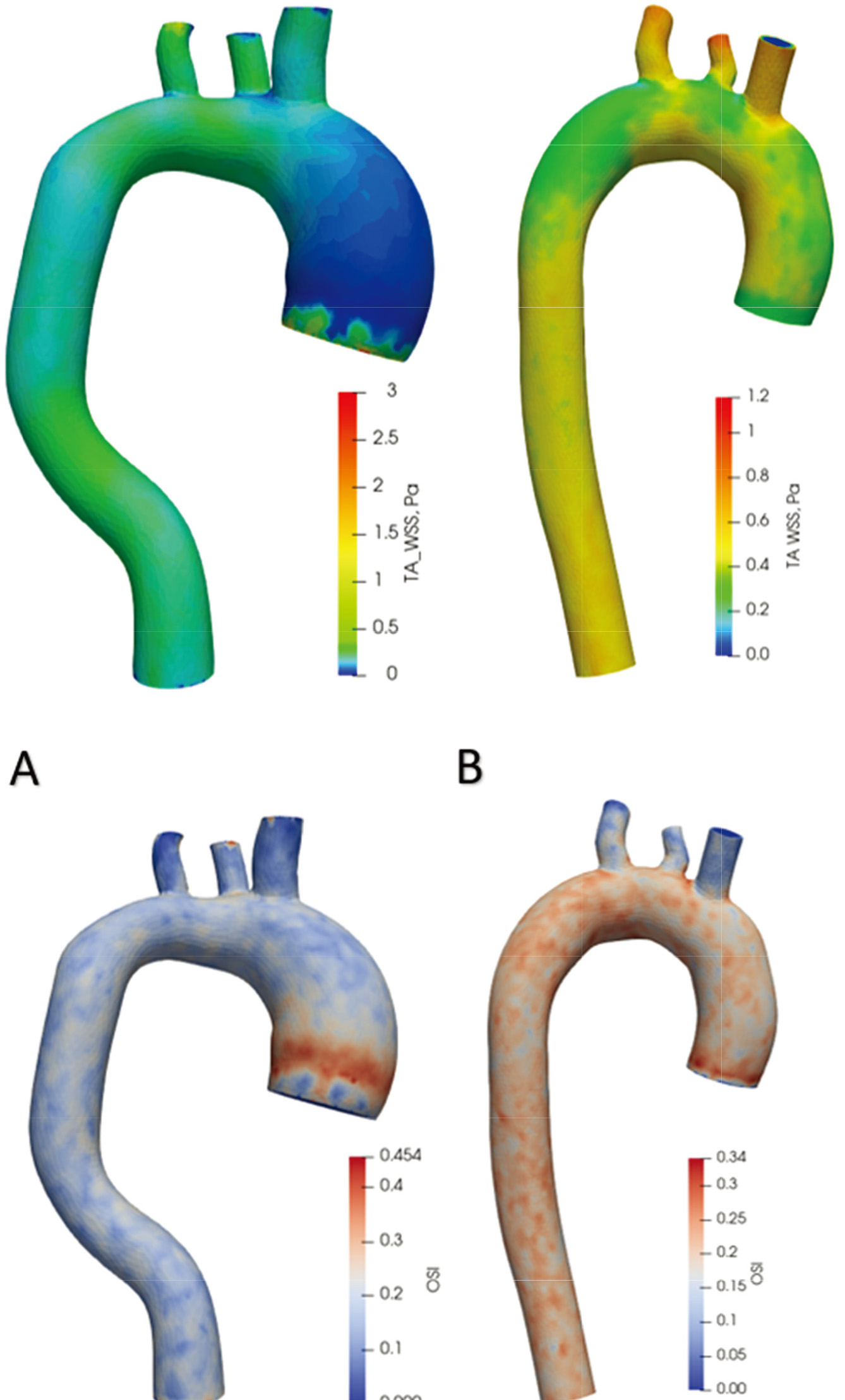
Time-averaged WSS and OSI views are shown in Fig. 10 over one cardiac cycle. In the aorta with an aneurysm, WSS values throughout the artery range from 0 Pa to 1 Pa. In comparison, in the healthy aorta, the distribution of values changes from 0.3 Pa to 0.6 Pa. In the aorta with an aneurysm, the highest OSI value (0.45) is at the onset of the aneurysm and then varies across the artery from 0.05 to 0.20. In a healthy aorta, OSI values vary uniformly across the artery from 0.15 to 0.30.
4.Discussion
4.1Flow rates
In the aorta with an aneurysm, the maximum blood flow velocity is almost 1.6 times lower than the systolic blood flow velocity in the healthy aorta. According to one study [30] where researchers measured flow velocities with an MRI scanner, the findings showed that the mean blood flow Q
4.2Pressure
The pressures obtained in this work show the normal pressure distribution during systole and diastole phases. The pressures are provided to verify that the modeling parameters (proximal and distal resistances) are selected correctly under the model outflow boundary conditions. In this study, it is not meaningful to compare pressure changes in a healthy aorta and in the aorta with an aneurysm, as the mean cardiac cycle pressure of 100 mm Hg was included in the calculation of boundary conditions (Eq. (4)).
4.3Displacement
The results obtained show that using the same boundary conditions, the value of wall displacements is 45% lower in a healthy aorta compared to an aorta with an aneurysm. This finding means that in the dilated aorta, the amplitude of wall movements increases during the cardiac cycle. In general, the greatest dilation of vascular walls occurs in the systolic phase, when the rate of blood inflow reaches its maximum value. In a previous study that examined aortic haemodynamic parameters in the presence of dissection, wall displacement before and after correction surgery were investigated. The study showed that in the case of arterial dissection, large wall displacements of 11 mm occurred due to arterial swelling and the resulting stresses. After aortic lumen correction, the displacements decreased to 0.5 mm [31]. In summary, displacements are also an important parameter indicating certain abnormalities and pathologies. Nevertheless, no studies to date have demonstrated any specific effects of displacements on aneurysm progression.
4.4WSS and OSI
In the presence of ascending aortic aneurysms, large areas of the low shear stress zone have been detected, as well as a corresponding increase in internal deformation of the aortic wall at that site. This case is characterised by a change in flow and a sudden drop in wall shear stresses in the aorta. In a study that examined blood flows in the aorta using MRI technology, the mean value of shear stresses in normal aortas was 1.5
Other researchers examined 224 aortas without pathologies [33] using four-dimensional flow MRI technology to determine wall shear stresses in a population of normal thoracic aortas. The mean peak systolic WSS was 1.79
In contrast to the studies described above, in this work, the same initial parameters were used for different aorta geometries, which shows how much the blood flow velocities and WSS/OSI distribution can differ in a healthy aorta and aorta with aneurysm under the same conditions.
4.5Limitations
The personalised geometry models analysed in this study use non-individualised parameters of blood flow and boundary conditions. The second limitation of this analysis is the small number of models. During the analysis, the blood was simulated as a Newtonian fluid, and the flow was assumed to be laminar. We encountered mesh problems because the SimVascular software uses a Tetgen mesh type and has limitations of mesh enhancement functions. This led to some distortion of the results such as high OSI values in the branches of aortic arch and distorted flow distribution within the aneurysm velocity profile. Future studies should be based on numerical modelling of fluid-structure interactions while considering the exact property of elasticity of the aortic wall and surrounding tissues from patient images. Although FSI analysis is more complex and requires more time and resources for modelling than simple CFD structural analysis or a coupled momentum method, the solutions obtained in FSI studies are more accurate. A patient-specific flow rate profile and turbulent flow modelling should be used to accurately assess blood flow and vascular stress and the associated risks of wall pathologies.
5.Conclusions
This study analysed the scientific literature on aortic pathologies. Two models of the thoracic aorta were designed using medical image segmentation: a normal aorta and an aorta with an ascending aneurysm. These artery models were analysed using the finite element method, and the results obtained were compared with each other and with prior results presented in scientific articles.
1. In aneurysms, the blood velocity is 1.6 times lower compared to a healthy aorta using same inlet boundary conditions. There is a difference in the distribution of flow velocity in the axial contour when comparing the aorta with the aneurysm to the healthy model. In the aneurysm zone, the flow rate slows down.
2. In an aorta with an ascending aneurysm, large changes in wall shear stresses occur, but the fluctuating shear index decreases by 33% compared to the results obtained from a healthy aorta.
3. An ascending aorta with an aneurysm demonstrates a 45% greater wall displacement compared to this part of the normal ascending aorta model. This finding means that the pathological aorta deforms more strongly during the cardiac cycle. This effect should be studied better in future research using more detailed aorta geometries including aortic root, valves, and annulus.
4. The methodology used in this study can be easily extended to a larger group of patients through a quantitative study to determine possible values for CFD modelling parameters in predicting aneurysm growth and rupture. The effect of blood flow on the distribution of aortic wall stresses will be useful for future studies to evaluate the effect of these types of distributions on the risk of aortic aneurysm rupture. In order to assess vascular changes qualitatively and accurately, the methodology should be improved using FSI, turbulent flow and patient-specific parameters.
Conflict of interest
None to report.
References
[1] | WHO. Cardiovascular diseases [Internet]. (2021) [cited 2021 Jun 17]. Available from: https://www.who.int/en/news-room/fact-sheets/detail/cardiovascular-diseases-(cvds). |
[2] | Dieter RS, Raymond A, Dieter J, Raymond A, Dieter I. Diseases of the Aorta. Springer International Publishing. (2019) ; 496. |
[3] | Saliba E, Sia Y. The ascending aortic aneurysm: When to intervene? IJC Hear Vasc. (2015) ; 6: : 91-100. doi: 10.1016/j.ijcha.2015.01.009. |
[4] | Yuan D, Luo H, Yang H, Huang B, Zhu J, Zhao J. Precise treatment of aortic aneurysm by three-dimensional printing and simulation before endovascular intervention. Sci Rep. (2017) ; 7: (1): 1-7. doi: 10.1038/s41598-017-00644-4. |
[5] | Ho D, Squelch A, Sun Z. Modelling of aortic aneurysm and aortic dissection through 3D printing. J Med Radiat Sci. (2017) ; 64: (1): 10-7. |
[6] | Gülan U, Calen C, Duru F, Holzner M. Blood flow patterns and pressure loss in the ascending aorta: A comparative study on physiological and aneurysmal conditions. J Biomech. (2018) ; 76: : 152-9. |
[7] | Marconi S, Lanzarone E, van Bogerijen GHW, Conti M, Secchi F, Trimarchi S, et al. A compliant aortic model for in vitro simulations: Design and manufacturing process. Med Eng Phys. (2018) ; 59: : 21-9. |
[8] | Amabili M, Balasubramanian P, Breslavsky I. Anisotropic fractional viscoelastic constitutive models for human descending thoracic aortas. J Mech Behav Biomed Mater. (2019) ; 99: (June): 186-97. doi: 10.1016/j.jmbbm.2019.07.010. |
[9] | Jiang DS, Yi X, Zhu XH, Wei X. Experimental in vivo and ex vivo models for the study of human aortic dissection: Promises and challenges. Am J Transl Res. (2016) ; 8: (12): 5125-40. |
[10] | Caballero AD, Laín S. A Review on Computational Fluid Dynamics Modelling in Human Thoracic Aorta. Vol. 4, Cardiovascular Engineering and Technology. Springer Science and Business Media, LLC; (2013) ; 103-30. |
[11] | Morris PD, Narracott A, Von Tengg-Kobligk H, Soto DAS, Hsiao S, Lungu A, et al. Computational fluid dynamics modelling in cardiovascular medicine. Heart. (2016) ; 102: (1): 18-28. |
[12] | Suito H, Takizawa K, Huynh VQH, Sze D, Ueda T. FSI analysis of the blood flow and geometrical characteristics in the thoracic aorta. (2014) . |
[13] | Raman RK, Dewang Y, Raghuwanshi J. A review on applications of computational fluid dynamics. (2018) . |
[14] | Dwidmuthe PD, Mathpati CS, Joshi JB. CFD Simulation of Blood Flow inside the Human Artery: Aorta. (2018) ; (January 2018): 1-5. |
[15] | Gray RA, Pathmanathan P. Patient-specific cardiovascular computational modeling: Diversity of personalization and challenges. J Cardiovasc Transl Res. (2018) ; 11: (2): 80-8. |
[16] | Borracci RA. Ascending aorta aneurysm – Thorax CTs – embodi3D.com [Internet]. (2019) [cited 2021 Jun 17]. Available from: https://wwwembodi3d.com/files/file/30284-ascending-aorta-aneurysm/. |
[17] | SimTK: SimVascular: Examples and Clinical Cases: Downloads [Internet]. [cited 2021 Jun 17]. Available from: https://simtkorg/frs/download_confirm.php/file/4301/AortofemoralNormal2.zip?group_id=930. |
[18] | Lan H, Updegrove A, Wilson NM, Maher GD, Shadden SC, Marsden AL. A Re-Engineered Software Interface and Workflow for the Open-Source SimVascular Cardiovascular Modeling Package. J Biomech Eng. (2018) ; 140: (2): 1-11. |
[19] | Schmidt R, Singh K. Meshmixer: An interface for rapid mesh composition. In: ACM SIGGRAPH 2010 Talks, SIGGRAPH ’10. (2010) . |
[20] | Hyochol A. SimVascular: An Open Source Pipeline for Cardiovascular Simulation. Physiol Behav. (2017) ; 176: (10): 139-48. |
[21] | Westerhof N, Lankhaar JW, Westerhof BE. The arterial windkessel. Vol. 47, Medical and Biological Engineering and Computing. Springer; (2009) ; 131-41. |
[22] | CPM Specifications Document Aortofemoral Normal. (2013) . |
[23] | Bonfanti M, Balabani S, Greenwood JP, Puppala S, Homer-Vanniasinkam S, Diáz-Zuccarini V. Computational tools for clinical support: A multi-scale compliant model for haemodynamic simulations in an aortic dissection based on multi-modal imaging data. J R Soc Interface. (2017) ; 14: (136). |
[24] | Si H. TetGen, a delaunay-based quality tetrahedral mesh generator. ACM Trans Math Softw. (2015) Jan 1; 41: (2). |
[25] | Figueroa A, Below ASD, Provided IS. SImVascular/Solver Users Manual. Work. (2008) . |
[26] | Ueda T, Suito H, Ota H, Takase K. Computational fluid dynamics modeling in aortic diseases. Cardiovasc Imaging Asia. (2018) ; 2: (2): 58. |
[27] | Gharahi H, Zambrano BA, Zhu DC, DeMarco JK, Baek S. Computational fluid dynamic simulation of human carotid artery bifurcation based on anatomy and volumetric blood flow rate measured with magnetic resonance imaging. Int J Adv Eng Sci Appl Math. (2016) ; 8: (1): 46-60. |
[28] | Fulker D, Ene-Iordache B, Barber T. High-resolution computational fluid dynamic simulation of haemodialysis cannulation in a patient-specific arteriovenous fistula. J Biomech Eng. (2018) ; 140: (3). |
[29] | Ahrens J, Geveci B, Law C. ParaView: An end-user tool for large-data visualization. In: Visualization Handbook. Elsevier Inc.; (2005) ; 717-31. |
[30] | Voges I, Jerosch-Herold M, Hedderich J, Pardun E, Hart C, Gabbert DD, et al. Normal values of aortic dimensions, distensibility, and pulse wave velocity in children and young adults: A cross-sectional study. J Cardiovasc Magn Reson. (2012) ; 14: (1). |
[31] | Qiao Y, Fan J, Ding Y, Zhu T, Luo K. A primary computational fluid dynamics study of pre-and post-tevar with intentional left subclavian artery coverage in a type b aortic dissection. J Biomech Eng. (2019) ; 141: (11): 1-8. |
[32] | Condemi F, Campisi S, Viallon M, Croisille P, Fuzelier JF, Avril S. Ascending thoracic aorta aneurysm repair induces positive hemodynamic outcomes in a patient with unchanged bicuspid aortic valve. J Biomech. (2018) ; 81: : 145-8. doi: 10.1016/j.jbiomech.2018.09.022. |
[33] | Callaghan FM, Grieve SM. Translational Physiology: Normal patterns of thoracic aortic wall shear stress measured using four-dimensional flow MRI in a large population. Am J Physiol – Hear Circ Physiol. (2018) ; 315: (5): H1174-81. |
[34] | Simao M, Ferreira JM, Tomas AC, Fragata J, Ramos HM. Aorta ascending aneurysm analysis using CFD models towards possible anomalies. Fluids. (2017) ; 2: (2): 1-15. |


