
Convolutional neural network-based surgical instrument detection
Abstract
BACKGROUND:
Minimally invasive surgery (MIS), unlike open surgery in which surgeons can perform surgery directly, is performed using miniaturized instruments with indirect but careful observation of the surgical site.
OBJECTIVE:
Instrument detection is a crucial requirement in conventional and robot-assisted MIS, which can also be very useful during surgical training. In this paper, we propose a novel framework of using two three-layer convolutional neural networks (CNNs) in a series to detect surgical instrument in in-vivo video frames.
METHODS:
The two convolutional neural networks proposed in this paper have different tasks. (i) The former CNN is trained to detect the edges points of the instrument shaft directly from images patches. (ii) The latter is trained to locate the instrument tip also from images patches after the former detection finishes.
RESULTS:
We validated our method on the publicly available EndoVisSub dataset and a standard dataset, and it detected tools with an accuracy of 91.2% and 75% respectively.
CONCLUSION:
Our two-step detection method achieves better performance than other existing approaches in terms of detection accuracy.
1.Introduction
Computer vision-based detection of surgical instruments in computer-assisted intervention (CAI) systems for MIS has received a great deal of attention recently [1]. This is largely due to the requirements for more accurate detection of surgical instruments, especially in robot-assisted systems [2, 3]. Compared with traditional open surgery, MIS has many advantages including less pain, less risk of infection and less blood loss. However, because of the indirect observation of the surgery site, it could be challenging for surgeons to carry out such a surgery. Under such conditions, locating instruments in the video can help surgeons to lighten their burden of finding the instruments during an operation, which is beneficial to both surgeons and patients.
In recent years, many image-based methods have been proposed to detect instruments in 2D or 3D. Conventional methods use low-level features to locate instruments in images [4]. For instance, Augustine and Voros [5] proposed a simple and robust algorithm to estimate the 2D/3D pose of instruments based on image processing. Another example is the study by Rieke et al. [6], which employed the RGB and HOG feature of the instrument for the detection task.
Powerful deep learning algorithms, which can learn hierarchical features through their structure and are widely used in the field of computer vision [7, 8], have become the mainstream methods in instrument tracking or detection. The modified and extended U-net [9] architecture was proposed by Kurmann et al. [10] for 2D vision-based recognition and pose estimation of multiple instruments, while the fully convolutional network [11] (FCN) was employed for tracking [12]. Due to the interdependence of location and segmentation of the surgical instrument, Laina et al. [13] proposed to use CSL model to perform instrument segmentation and pose estimation simultaneously. The fast RCNN [14] was also used to output a bounding box of surgical instruments but not a precise location with a region proposal network (RPN [15]). Moreover, to get a more precise location, more than one convolutional neural network may be used in some detection methods. Mishra et al. [16] proposed a deep learning approach based on late fusion CNN responses over pyramidally decomposed frames to locate the instrument tip. The network used above is deep and it is hard to train. We aimed to find a method using CNN of fewer layers that makes it easier to solve the detection problem.
In this paper, we propose a method based on two three-layer networks. The surgical instrument in MIS is usually rigid and straight, so we propose to use a two-step method that firstly detects the edges of the instrument and then the instrument tip will be predicted along its mid axis, which is the diagonal line of the two detected straight edge lines. As for the first step, edges detection, there are many methods that can be used. Comparing the edge detection using CNN [17] with other three edge detection methods [18, 19, 20], we finally decided to apply CNN to detect the edges in this paper. Edge detection using CNN is simple and efficient and, more importantly, is easy to implement. The next step is tip location. Because we know that the instrument tip is on the mid axis of the instrument, another CNN which has the same architecture as the former one is trained to determine the instrument tip, and both CNNs are trained in an end-to-end fashion. We validated our method on the EndoVisSub dataset and a standard dataset, and it shows good performance in terms of location accuracy.
The paper is organized as follows. In Section 2, we explain our method in detail. In Section 3, the experiments and results are given. Section 4 concludes this paper.
2.Surgical instrument detection method
2.1Instrument detection model
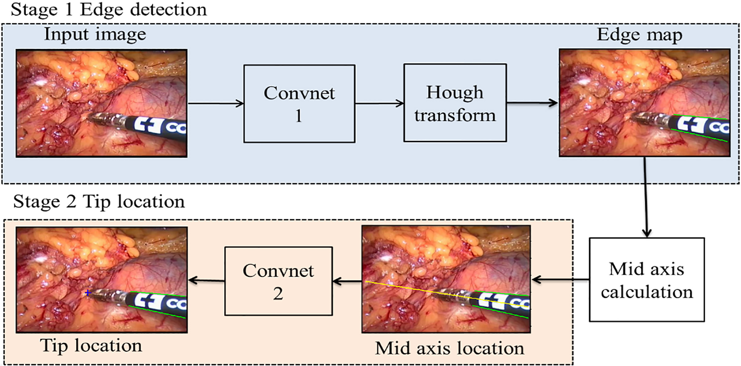
The structure of surgical instruments in an image frame can be viewed as two parts that are a straight shaft and an articulated end-effector [1]. In light of this, we divided our detection process into two main stages. As shown in Fig. 1, our detection system has two CNN in series and some image processing methods are applied in it. The two main stages are as follows: (i) Stage 1, detect the two edges of the instrument using a trained CNN followed by Hough transform [21] and then get the mid axis which is the diagonal line of two straight edges. (ii) Stage 2, locate the instrument tip based on a CNN along the mid axis. Although these two CNNs have the same architecture, they are trained separately.
Figure 1.
The framework of the proposed detection method. The green lines are the predicted edges of the instrument, and the yellow line represents its mid axis in this video frame. The predicted instrument tip location is marked by a red colored ‘
2.2Edge detection of the instrument
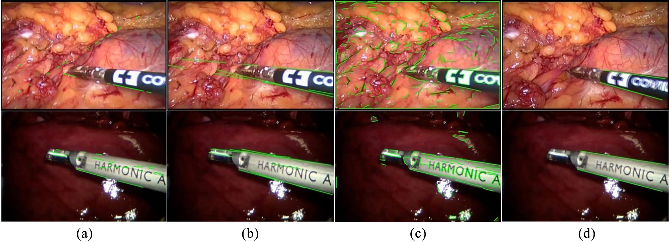
In stage 1, two straight edges of the instrument are detected by edge detection sub-network. There are many edge detection methods, such as canny edge detection, structure forest and line segment detection, as shown in Fig. 2. Because of the complex background and other disturbing factors, (a), (b) and (c) can hardly get the two straight edges of the shaft as we want it, and there are always more than two detected edge lines. Therefore, our method is more satisfying under such condition. Our detector takes an RGB video frame as input and predicts edge points that make up the edge map, and then using Hough transform we get two straight edge lines of the instrument shaft.
Figure 2.
Different edge detection methods: (a) Canny edge detection and Hough transform, (b) structured forest, (c) line segment detector (LSD) and (d) our method. The datasets from top to bottom are the Endovissub dataset and the standard dataset.
The architecture of CNN used in both stages is shown in Fig. 3. It consists of two convolutional layers, two rectified linear units (ReLU), a fully connected (fc) layer and a softmax layer. Compared with traditional CNN architecture, the pooling layer is removed, but it does not influence the accuracy of our detection. The network outputs a discrete probability
(1)
where
Figure 3.
Architecture of the CNN used in the proposed method
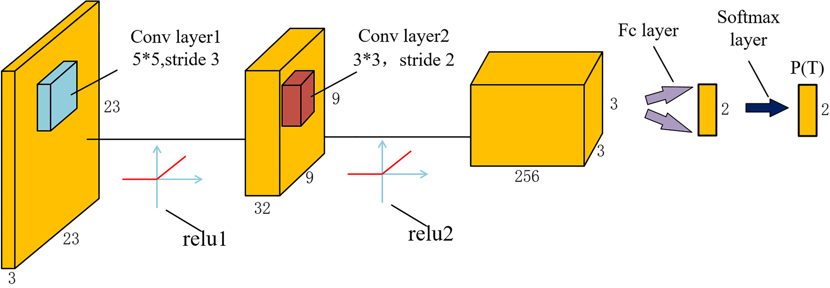
In our approach, instrument edge detection in the RGB image is regarded as a classification problem that patches of size 23*23*3 centered at points are labeled as edge patches or background patches, and their central points are either edge points or background points. We train the network using a cross-entry loss function:
(2)
where
While testing, Convnet1 takes patches of size 23*23*3 as the input image and makes predictions on whether their centers are edge points or background points, and then the edge map made of edge points is predicted after all the edge points are found in that frame. As we aimed to get two straight edge lines of the instrument shaft, we applied Hough transform to produce the final edge map.
2.3Tip location of the instrument
In stage 2, the instrument tip is predicted by Convnet2. This network has the same architecture as that used in stage 1. The difference is that patches of size of 23*23*3 which fed into Convnet2 are labeled as instrument tip patch or background patches, and their central point is either instrument tip or background point during training period.
As seen in Fig. 1, along the mid axis which is the diagonal line of the two straight edge lines, the instrument tip is detected by Convnet2. We know that the instrument tip is on this mid axis, so we select the patches of which the central pixels are on the mid axis and feed them into Convnet2 to get the predicted probabilities of being instrument tip. Lastly, we can determine the instrument tip on whether it has the highest probability.
3.Experiment and results
3.1Data preparation and CNN training
To validate the proposed method, we compared our method to three other methods on two benchmark datasets. These are the EndoVisSub dataset [22] (300 frames of size 640*480) and the standard dataset [23] (400 frames of size 640*480). Before getting the training patches, we resized these video frames into 481*321 pixels. Then we divided these video frames into three subparts, 80% of frames for training and the rest 20% for testing. The ground truth annotations of the instrument tip and edge map, which were saved in the form of 2D coordinates, are available for analysis and comparison.
Figure 4.
Examples of patches used for training. ‘P’ represents positive sample and ‘N’ represents negative sample.
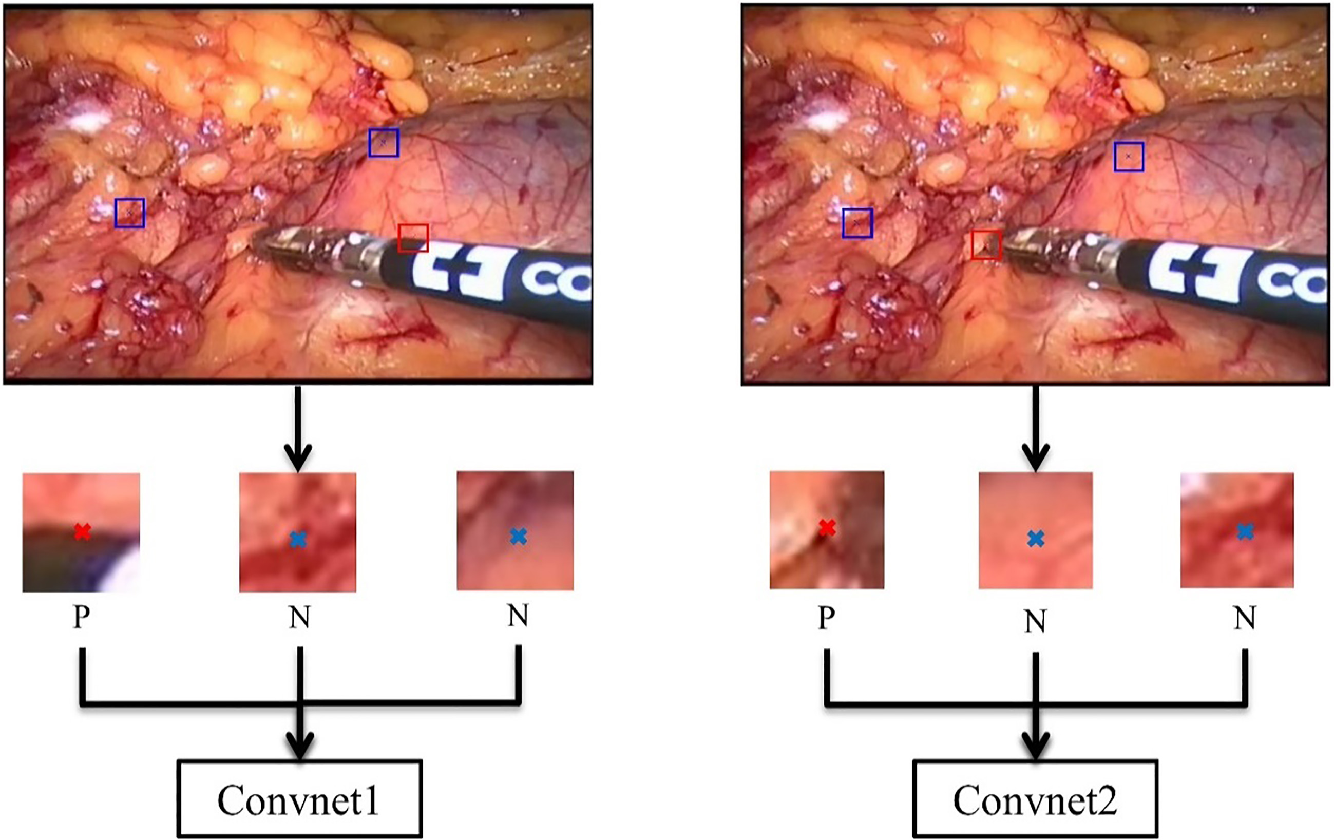
As shown in Fig. 4, the left one is the training framework for Convnet1 and the right one for Convnet2. In order to obtain patches as positive samples for the training, we cropped every video frame into patches of size of 23*23*3 of which the centers are ground-truth annotations colored in red ‘x’ in the figure. As for negative samples, we obtained patches whose center are colored in blue ‘x’ in the figure, which does not locate on the edge map or instrument tip. However, there are so many negative samples that we cannot select all of them in a video frame. We therefore selected a part of negative patches randomly and then fed these negative/positive patches into the Convnet for training.
To evaluate the performance of the method, we compared it to three other methods. The methods we chose are: locating instrument tip directly by Convnet2-based traditional sliding window method (SWM) [24], tracking with an active filter (AF) [25], and scale invariant deep learning-based detection approach (SIDL) [16]. These methods were all implemented in Matlab.
We used the Matconvnet toolbox of Matlab to train both of our networks on CPU. Convnet1 was trained with stochastic gradient descent (SGD) over 20 epochs with a learning rate of 10
3.2Results
The test video images using our two-stage method for two datasets are shown in Fig. 5. There are several disturbing factors in the test frames, such as illumination changing, motion blur and complex operating background which sometimes make the detector cause bigger errors.
Figure 5.
Test examples of each method. Approches from left to right are SWM [24], AF [25], SIDL [16] and our method. The top row represents the EndoVisSub dataset, and the bottom row represents the standard dataset.
![Test examples of each method. Approches from left to right are SWM [24], AF [25], SIDL [16] and our method. The top row represents the EndoVisSub dataset, and the bottom row represents the standard dataset.](https://content.iospress.com:443/media/thc/2020/28-S1/thc-28-S1-thc209009/thc-28-thc209009-g005.jpg)
In order to evaluate the proposed method, for each testing image we compared the predicted tip location to its manual annotation. The accuracy rates of four detectors are presented in Table 1. If the distance between the predicted position and the ground truth is larger than 20 pixels in the frame image coordinate system, we think the detector has lost the object in this frame.
Table 1
Accuracy rates for every method on every dataset
| [height=0.8cm,width=2.4cm]DatasetMethods | SWM | AF | SIDL | Ours |
|---|---|---|---|---|
| Endovissub dataset | 35% | 66.7% | 68.3% | 75% |
| Standard dataset | 48.8% | 80% | 86.3% | 91.2% |
3.3Comparison of different configurations
We also tried different network structures and the size of image patches in our experiments. Table 2 compares the performance while using different networks by adding a pooling layer or another convolutional layer and different input sizes which are 17*17*3, 23*23*3 and 29*29*3. However, as shown in Table 2, adding a convolutional layer or pooling layer and using different input sizes can hardly improve the performance. It shows that the networks used in our method are sufficient for this detection problem.
Table 2
Performance comparison when using different configurations. C represents convolutional layer, P and F are pooling layer and fully connected layer respectively
| Convnet1 | Convnet2 | Orientation error | Accuracy rate | ||
|---|---|---|---|---|---|
| Network | Patch size | Network | Patch size | ( | (%) |
| CCF | 23*23*3 | CCF | 23*23*3 | 0.35 (0.25) | 91% |
| CCF | 23*23*3 | CCCF | 23*23*3 | 0.35 (0.25) | 90% |
| CCF | 29*29*3 | CCF | 23*23*3 | 0.45 (0.52) | 87% |
| CCF | 17*17*3 | CCF | 23*23*3 | 0.88 (0.62) | 88% |
| CCCF | 23*23*3 | CCF | 23*23*3 | 0.40 (0.45) | 88% |
| CCF | 23*23*3 | CPCF | 23*23*3 | 0.35 (0.25) | 85% |
| CCF | 23*23*3 | CCF | 17*17*3 | 0.35 (0.25) | 89% |
| CCF | 23*23*3 | CCF | 29*29*3 | 0.35 (0.25) | 87% |
| CPCF | 23*23*3 | CCF | 23*23*3 | 0.58 (0.63) | 86% |
4.Conclusion
In this paper, we proposed a deep-learning method for instrument detection. Two CNNs of the same architecture were used but they had different tasks. Convnet1 in stage 1 was trained to predict the edge map of the instrument shaft, and Convnet2 in stage 2 was trained for tip location. Unlike previous work, the architecture of the CNN used in this work is simple, which makes our method easier to implement. Furthermore, the comparison experiment shows that our detector can locate the instrument tip with high accuracy and also proves that edge detection in stage 1 is the dispensable part in our method. Finally, we tried different networks and different patch sizes, but we found that they cannot improve the performance. As for the shortcomings, we should mention that the image blurring caused by the instrument’s fast moving can lead to bad detection results, and our method is limited to a straight instrument.
Detecting the surgical instrument in images is a challenging task, because there are always many disturbing factors. For example, when multiple instruments are present, a part of them may be occluded, which can badly influence the tip detection. We will work on solving these challenges and limitations of our method in the future.
Conflict of interest
None to report.
References
[1] | Wesierski D, Wojdyga G, Jezierska A. Instrument tracking with rigid part mixtures model. Computer-Assisted and Robotic Endoscopy. Cham: Springer; (2015) ; p. 22-34. |
[2] | Wang W, Shi Y, Goldenberg AA. et al. Experimental analysis of robot-assisted needle insertion into porcine liver. Bio-Medical Materials and Engineering. (2015) ; 26: (s1): S375-S380. |
[3] | Wang WD, Zhang P, Shi YK, et al. Design and compatibility evaluation of magnetic resonance imaging-guided needle insertion system. Journal of Medical Imaging and Health Informatics. (2015) ; 5: (8): 1963-1967. |
[4] | Rieke N, Tan DJ, Alsheakhali M, et al. Surgical tool tracking and pose estimation in retinal microsurgery. International Conference on Medical Image Computing and Computer-Assisted Intervention. Cham: Springer; (2015) ; p. 266-273. |
[5] | Agustinos A, Voros S. 2D/3D real-time tracking of surgical instruments based on endoscopic image processing. Computer-Assisted and Robotic Endoscopy. Cham: Springer; (2015) ; p. 90-100. |
[6] | Rieke N, Tan DJ, di San Filippo CA, et al. Real-time localization of articulated surgical instruments in retinal microsurgery. Medical Image Analysis. (2016) ; 34: : 82-100. |
[7] | Redmon J, Divvala S, Girshick R, et al. You only look once: Unified, real-time object detection. Proceedings of the IEEE conference on computer vision and pattern recognition; Las Vegas: IEEE; (2016) ; p. 779-788. |
[8] | Simonyan K, Zisserman A. Two-stream convolutional networks for action recognition in videos. Advances in neural information processing systems. Montreal, Canada; (2014) ; p. 568-576. |
[9] | Ronneberger O, Fischer P, Brox T. U-net: Convolutional networks for biomedical image segmentation. International Conference on Medical image computing and computer-assisted intervention. Cham: Springer; (2015) ; pp. 234-241. |
[10] | Kurmann T, Neila PM, Du X, et al. Simultaneous recognition and pose estimation of instruments in minimally invasive surgery. International Conference on Medical Image Computing and Computer-Assisted Intervention. Canada: Springer, (2017) ; pp. 505-513. |
[11] | Long J, Shelhamer E, Darrell T. Fully convolutional networks for semantic segmentation. Proceedings of the IEEE conference on computer vision and pattern recognition. Boston: IEEE; (2015) ; pp. 3431-3440. |
[12] | García-Peraza-Herrera LC, Li W, Gruijthuijsen C, et al. Real-time segmentation of non-rigid surgical tools based on deep learning and tracking. International Workshop on Computer-Assisted and Robotic Endoscopy. Greece: Springer; (2016) ; pp. 84-95. |
[13] | Laina I, Rieke N, Rupprecht C, et al. Concurrent segmentation and localization for tracking of surgical instruments. International conference on medical image computing and computer-assisted intervention (2017) ; Canada: Springer; (2017) . pp. 664-672. |
[14] | Sarikaya D, Corso JJ, Guru KA. Detection and localization of robotic tools in robot-assisted surgery videos using deep neural networks for region proposal and detection. IEEE Transactions on Medical Imaging (2017) ; 36: (7): 1542-1549. |
[15] | Ren S, He K, Girshick R, et al. Faster r-cnn: Towards real-time object detection with region proposal networks. IEEE Transactions on Pattern Analysis and Machine Intelligence. (2017) ; 39: (6): 1137-1149. |
[16] | Mishra K, Sathish R, Sheet D. Tracking of Retinal Microsurgery Tools Using Late Fusion of Responses from Convolutional Neural Network over Pyramidally Decomposed Frames. International Conference on Computer Vision, Graphics, and Image processing. Cham: Springer; (2016) ; pp. 358-366. |
[17] | Wang R. Edge detection using convolutional neural network. International Symposium on Neural Networks. St. Petersburg, Russia: Springer; (2016) ; pp. 12-20. |
[18] | Canny J. A computational approach to edge detection. Readings in computer vision. Morgan Kaufmann; (1987) ; 184-203. |
[19] | Dollár P, Zitnick CL. Structured forests for fast edge detection. Proceedings of the IEEE international conference on computer vision. Sydney: IEEE; (2013) ; pp. 1841-1848. |
[20] | Von Gioi RG, Jakubowicz J, Morel JM, et al. LSD: A fast line segment detector with a false detection control. IEEE Transactions on Pattern Analysis and Machine Intelligence. (2008) ; 32: (4): 722-732. |
[21] | Duda RO, Hart PE. Use of the Hough transformation to detect lines and curves in pictures. Communications of the ACM. (1972) ; 15: (1): 11-15. |
[22] | MICCAI https//endovissub-instrument.grand-challenge.org/download/. |
[23] | Du X, Allan M, Dore A, et al. Combined 2D and 3D tracking of surgical instruments for minimally invasive and robotic-assisted surgery. International Journal of Computer Assisted Radiology and Surgery. (2016) ; 11: (6): 1109-1119. |
[24] | Dalal N, Triggs B. Histograms of Oriented Gradients for Human Detection. 2005 IEEE Computer Society Conference on Computer Vision and Pattern Recognition (CVPR’05). IEEE; (2005) . |
[25] | Sznitman R, Richa R, Taylor RH, et al. Unified Detection and Tracking of Instruments during Retinal Microsurgery. IEEE Transactions on Pattern Analysis and Machine Intelligence. (2013) ; 35: (5): 1263-1273. |


