
Ventricular repolarization instability quantified by instantaneous frequency of ECG ST intervals
Abstract
BACKGROUND:
Ventricular repolarization instabilities have been documented to be closely linked to arrhythmia development. The electrocardiogram (ECG) ST interval can be used to measure ventricular repolarization. Analyzing the duration variation of the ST intervals can provide new information about the arrhythmogenic vulnerability.
OBJECTIVE:
In this work, we propose a new method based on mean instantaneous frequency (IF) of the ST intervals to quantitatively evaluate the risk of sudden cardiac deaths (SCDs).
METHODS:
Two spectral bands, i.e. the low-frequency band (LF, 0–0.15 Hz) and the high-frequency band (HF, 0.15–0.5 Hz), are considered in this paper. Based on IF estimates, the ECG recordings from three MIT-BIH databases that represent different risk levels of SCD occurrence are used, and their mean IFs in the LF and HF bands are calculated.
RESULTS:
The statistical results show that healthy subjects have a higher mean IF in the HF band and a lower mean IF in the LF band. The experimental results are the opposite for patients with malignant ventricular arrhythmia.
CONCLUSION:
The proposed mean IF can represent an indirect measure of intrinsic ventricular repolarization instability and can mark cardiac instability associated with SCDs.
1.Introduction
Sudden cardiac death (SCD) is a major cause of death around the world. Ventricular arrhythmias, such as ventricular tachycardia/fibrillation, mostly cause SCDs. Currently, antiarrhythmic drugs and implantable cardioverter defibrillators (or a combination of them) are widely used to treat cardiac arrhythmias and eventually prevent SCDs. However, they should be assessed on patient safety, and their use is costly [1]. Ventricular repolarization analysis based on the surface electrocardiogram (ECG) is a low-cost, noninvasive approach that has shown to be useful for the risk assessment of SCD and can be applied to the general population. Instabilities in ventricular repolarization have been documented to be closely linked to arrhythmia development, and are regarded as a harbinger of malignant arrhythmias [1].
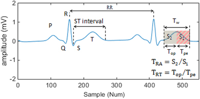
Ventricular repolarization instability (VRI) includes spatial and temporal repolarization heterogeneities. For an ECG marker for spatial repolarization instability, QT dispersion [2] is considered to reflect the instability on ECG intervals. Several other indices have also been proposed to define the T-wave shape [3, 4], such as T-wave amplitude (T
Figure 1.
Terminologies related to the T-wave.
In [5], QT variations from the proportion to HR variations were assessed by considering the following log-ratio index:
(1)
where QT
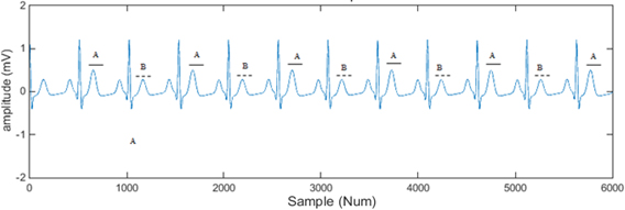
T-wave alternans (TWA) is proposed as an ECG marker for the characterization of spatio-temporal repolarization instability. TWA refers to a repeated ABAB pattern in amplitude or the shape of ST-T complex as shown in Fig. 2. It has been proposed as an independent index of susceptibility to ventricular arrhythmias, and has been used in some aspects of clinical evaluation [6, 7].
Figure 2.
An example of T-wave alternans.
There are some other approaches that assess repolarization variability using parametric modeling [8, 9]. However, most of the above methods are only used in the context of research studies and have not yet bridged the gap to clinical routines. The effectiveness and stability of the methods are key issues that need to be improved. Translation of the information of the ventricular repolarization phase into valuable clinical decision-making tools remains a challenge.
For healthy people, patients with arrhythmias, and patients with malignant arrhythmias, their degree of VRI varies, and generally speaking their risk of sudden cardiac death gradually increases. In this work, the ST interval of the ECG signal is used to quantify VRI and assess the SCD risk. The ST interval (see Fig. 1) is measured from the end of S-wave to the end of the T-wave. It represents the duration in which the ventricles repolarize. The alterations of this period of a heart cycle are an important factor for arrhythmogenesis that may induce lethal ventricular arrhythmias. Analyzing the variation of the duration of the ST intervals can provide new information about the arrhythmogenic vulnerability.
ECG signals are nonstationary processes in nature. To present the nonstationarity, time-frequency analysis techniques are suitable tools since they can represent signals simultaneously in both time and frequency. In this work, the instantaneous frequency (IF), which is estimated based on Hilbert transform (HT), is applied to analyze ST interval signals.
The remainder of this paper is organized as follows. In Section 2, we describe the data used in this work, the processing method and the Hilbert transform-based IF analysis. In Section 3, we report the experimental results. In Section 4, we provide statistical analysis and discuss the limitations. Finally, we provide a summary of conclusions in Section 5.
2.Materials and methods
2.1Materials
The MIT-BIH database (http://www.physionet.org/data) provided by the Massachusetts Institute of Technology is currently the most widely used database in the research area. In this work, three sub-databases from the MIT-BIH database are chosen [10]: MIT-BIH Normal Sinus Rhythm Database (NSR db), MIT-BIH Arrhythmia Database (Arrhythmia db), and MIT-BIH Malignant Ventricular Arrhythmia Database (MVA db).
The NSR db includes 18 long-term ECG recordings recorded in the Arrhythmia Laboratory at the Beth Israel Deaconess Medical Center. The subjects included in the database were five men, aged 26 to 45, and 13 women, aged 20 to 50. They did not have significant arrhythmias.
The Arrhythmia db contains 48 half hour excerpts from two-channel ambulatory ECG recordings, obtained from 47 subjects studied in the BIH Arrhythmia Laboratory. Twenty-three recordings were chosen at random from a set of 4000 24 hour ambulatory ECG recordings collected from a mixed population of inpatients and outpatients at Boston’s Beth Israel Hospital. The remaining 25 recordings were selected from the same set to include less common but clinically significant arrhythmias.
The MVA db includes 22 half hour ECG recordings from subjects who experienced episodes of sustained ventricular tachycardia, ventricular flutter, and ventricular fibrillation. To some extent, the chosen ECG data from the three databases represent the different risk levels of occurring malignant heart events. They were recorded from lower level to high risks subjects.
A total of 48 sets of records, including 13 sets from the NSR db, 15 sets from the Arrhythmia db, and the 18 sets from MVA db, were used for the experiments. The other records from the three databases were discarded because of their poor signal quality. All data length was below 10 minutes. For the MVA db, all subjects experienced a sudden cardiac death within 24 hours.
2.2Methodology
Prior to computing the ECG repolarization index (ST interval), the following processing steps were applied.
2.2.1ECG preprocessing
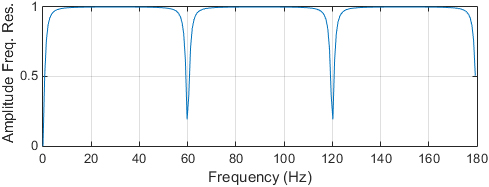
This step includes the removal of power line interference and baseline wander (BW) [11]. The comb filter [12] and wavelet and morphological filters [13, 14] are used to suppress the power line interference and BW, respectively. In practice, many filters such as the Kalman filtering and state filtering [15, 16, 17, 18] have been used in signal processing, state estimation, system modeling and parameter identification [19, 20, 21]. Different signals have different frequency characteristics. According to the signal frequency distributions, high-pass filters or low-pass filters can be designed to remove the disturbance noise in signals. Some parameter estimation methods can be used for modeling the signals from observation data by means of the iterative search and optimization strategies [22, 23, 24].
A comb filter passes all frequencies except those in a stop band centered on a center frequency. We cascaded a digital notching filter with order 10 and the width of the filter notch at
Figure 3.
The amplitude-frequency characteristics curve of the comb filter.
An effective method that combines mathematical morphological filtering (MMF) and wavelet transform (WT) techniques is used to suppress BW. The entire block diagram of the combined algorithm is shown in Fig. 4.
Figure 4.
The wavelet and morphological filter suppressing BW noise.
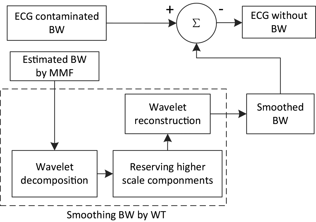
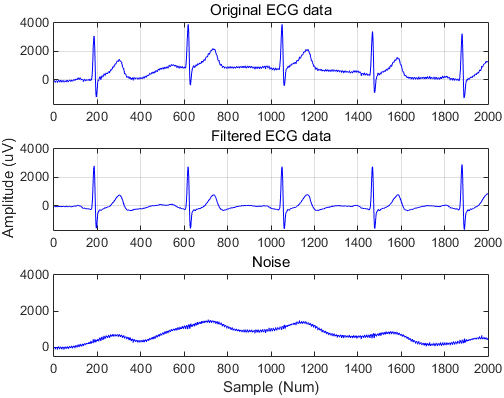
Considering the distortions caused by MMF, wavelet transform follows to smooth the estimated BW, which can improve the signal-to-noise ratio. In this work we chose coif3 as the wavelet function for its regularity and symmetry properties. An example of ECG preprocessing is given in Fig. 5.
Figure 5.
An example of ECG noise suppression.
2.2.2Wave delineation
The most relevant points for repolarization analysis are the QRS boundaries, T-wave boundaries, and T-wave peak. Prior to the determination of the ST intervals, the peaks of the QRS complex and T-waves are accurately localized. For ECG delineation, algorithms are often used to define temporal search windows before and after the QRS fiducial points to determine other wave patterns. Once the search window is defined, relevant techniques are applied to enhance the characteristic features of each wave in order to determine the wave peaks and boundaries [25, 26].
Figure 6.
Automatic determination of the peaks of R- and T-waves by a wavelet-based method.
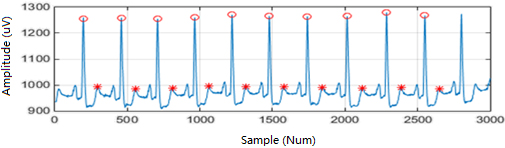
Figure 7.
Automatic localization of S- and T-wave boundaries by a wavelet-based method.
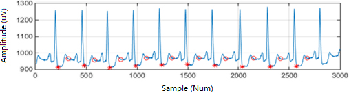
In this work, a wavelet-based ECG delineator is applied to automatically determinate the peaks of the R- and T-wave, and then localize the S- and T-wave boundaries [27]. A quadratic spline is used as the prototype wavelet. QRS complexes are detected by searching across the scales for ‘maximum modulus lines’ exceeding some thresholds at scales. The zero crossing of the WT at some scales between a positive maximum-negative minimum pair is marked as a QRS. Then, the peaks of the QRS individual waves (R, S) are identified, as well as the complex onset and end. They are based on the presented slope and local minimum criteria. Finally, the determination of T-wave peaks, onsets and ends is performed. A search window for each beat is defined and within this window we look for local maxima of some higher scales. If at least two of them exceed the threshold, a T-wave is considered to be present. To identify the T-wave boundaries, the same criteria as for the QRS onset and end are used. Examples of ECG wave delineation are given in Figs 6 and 7.
2.2.3Segmentation
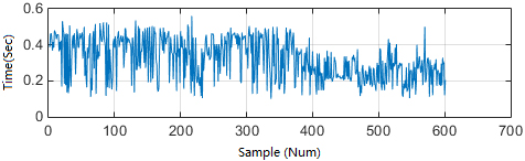
An ST interval is considered a repolarization segmentation window in this work. It contains the ST-T complex. The repolarization segments are extracted from each beat of an ECG recording to form the ST interval serials. An example of the extracted ST interval serials is given in Fig. 8. The unevenly time serial signals are processed using cubic spline interpolation and sampled at 1 Hz prior to applying the following temporal-frequency analysis.
Figure 8.
The extracted ST interval serials of recording no. 427 from the MVA db.
2.3Instantaneous frequency analysis of ECG ST intervals
An ST interval represents a complete duration of ventricular repolarization, and ST interval time series are essentially nonstationary, which means that the statistical properties of the signals often change over time. The instantaneous frequency (IF) of cardiovascular time series is used to describe the time-varying spectral contents of the characteristic frequency bands that are of interest to psychophysiological and cardiovascular research [28].
HT is applied to obtain IF components of the ST interval series. Given a real time function
(2)
The concept of an analytic signal or pre-envelope of a real signal
(3)
and its instantaneous phase angle in the complex plane can be defined by:
(4)
Then, the IF of
(5)
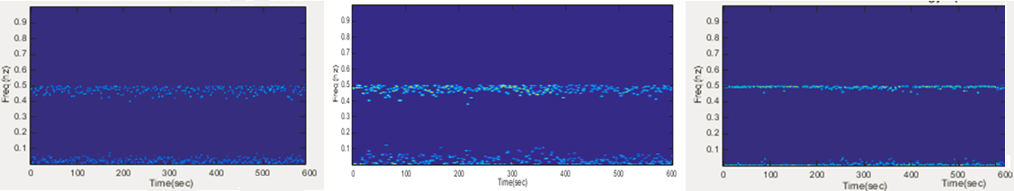
An example of the temporal-frequency diagrams of recording no. 18184 from NSR db, no. 103 from Arrhythmia db, and no. 427 from MVA db are given in Fig. 9, respectively.
Figure 9.
An example of the temporal-frequency diagrams of ECG recordings from three different databases. (a) Recording no. 18184, (b) recording no. 103 (c), and recording no. 427.
The IF of a signal often produces results that are paradoxical in some way [30], and make it difficult to interpret physically. In this work, the drawbacks are overcome by calculating the mean IF. Usually, on the basis of spectral analysis, these fluctuations are divided into two characteristic spectral ranges: the low-frequency (LF) range of 0.0–0.15 Hz, and the high-frequency (HF) range of 0.15–0.50 Hz [31, 32, 33]. The two frequency ranges are used in this work.
3.Results
For the time-frequency distributions, the mean IF of the ST intervals from each ECG recording in the HF and LF bands is calculated, and the results are shown in Table 1. As can be seen, in the HF band, the ECG data from the NSR db have the highest mean IF (0.4943
Table 1
The mean IF of the ST intervals from the ECG records from the databases
| MVA db | HF | LF | Arrhythmia db | HF | LF | NSR db | HF | LF |
|---|---|---|---|---|---|---|---|---|
| 419 | 0.4916 | 0.0081 | 101 | 0.4927 | 0.0078 | 16265 | 0.4923 | 0.0102 |
| 421 | 0.4788 | 0.0191 | 103 | 0.4959 | 0.004 | 16272 | 0.4902 | 0.0122 |
| 424 | 0.4794 | 0.0212 | 105 | 0.492 | 0.0095 | 16420 | 0.4818 | 0.0213 |
| 425 | 0.4748 | 0.022 | 111 | 0.4911 | 0.0081 | 16483 | 0.4973 | 0.0035 |
| 426 | 0.4806 | 0.0205 | 115 | 0.4908 | 0.0084 | 16539 | 0.4941 | 0.0075 |
| 427 | 0.4745 | 0.0249 | 201 | 0.4877 | 0.0163 | 16773 | 0.4971 | 0.0029 |
| 428 | 0.4811 | 0.0168 | 203 | 0.4836 | 0.0203 | 16786 | 0.4984 | 0.0015 |
| 429 | 0.4854 | 0.0158 | 208 | 0.4888 | 0.014 | 16795 | 0.4941 | 0.0051 |
| 430 | 0.4714 | 0.0224 | 215 | 0.4936 | 0.006 | 18177 | 0.4975 | 0.003 |
| 602 | 0.4783 | 0.0129 | 217 | 0.4923 | 0.0089 | 18184 | 0.4956 | 0.0055 |
| 605 | 0.4682 | 0.0252 | 221 | 0.483 | 0.0232 | 19088 | 0.4943 | 0.0038 |
| 607 | 0.478 | 0.0215 | 222 | 0.4737 | 0.0189 | 19090 | 0.4957 | 0.0037 |
| 609 | 0.4649 | 0.0173 | 223 | 0.4928 | 0.0067 | 19093 | 0.4978 | 0.0027 |
| 610 | 0.4775 | 0.0233 | 230 | 0.4916 | 0.0087 | |||
| 611 | 0.4776 | 0.0242 | 233 | 0.4939 | 0.005 | |||
| 612 | 0.4817 | 0.0159 | ||||||
| 614 | 0.4703 | 0.0249 | ||||||
| 615 | 0.4752 | 0.0182 | ||||||
| Mean | 0.4772 | 0.0197 | Mean | 0.4896 | 0.0111 | Mean | 0.4943 | 0.0064 |
| 0.0062 | 0.0046 | 0.0057 | 0.0060 | 0.0044 | 0.0055 |
Figure 10.
The mean IF distributions of the ECG recordings from the three databases.
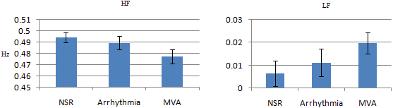
In the HF band, most ECG records from the NSR db have a higher mean IF, compared to other ECG records from the Arrhythmia and MVA db, while in the LF band, most records from the MVA db have a higher mean IF.
4.Statistical analysis
Two-sample
Table 2
Significant difference of the results for the NSR db, Arrhythmia db and MVA db
| Sample ECG source | HF | LF |
|---|---|---|
| NSR db | ||
| MVA db | ||
| NSR db | ||
| Arrhythmia db | ||
| MVA db | ||
| Arrhythmia db |
The mean IFs of the ECG data from the MVA db and Arrhythmia db both are significantly different from those of the ECG data from the NSR db, whether in the HF or LF bands. In fact, differences were also found in the mean IFs between the ECG recordings from the MVA db and the Arrhythmia db. Generally speaking, healthy people have a lower risk of developing SCDs, whereas patients with frequent arrhythmic events have a higher risk of having SCDs and patients with malignant ventricular arrhythmia are highly likely to have a SCD.
In this work, the subjects were chosen from three different databases, which represent different groups of people, and the data were collected using different sampling rates (128 Hz for NSR db, 360 Hz for Arrhythmia db, and 250 Hz for MVA db), but the similar laws of HF and LF (despite the opposite trend) of mean IF are shown. Although the sample size in the investigation is not very large, the mean IF shows a high degree of consistency with the above phenomena, which demonstrates that the smaller mean IF in the HF band, the higher the risk of having a SCD. Similarly, the higher the mean IF in the LF band, the higher the risk of having a SCD. The statistical results in terms of the significance show the effectiveness of using the mean IF as a risk-stratifier of SCD.
5.Conclusion
To some extent, the ECG data from the NRS, Arrhythmia, and MVA databases represent different risks of heart diseases. In particular, the records from the MVA database are half hour excerpts of sudden cardiac deaths, and the Holter database, a collection of long-term ECG recordings of patients who experienced sudden cardiac deaths during the recordings. The ST intervals of an ECG signal represent the durations of ventricular repolarization. Our works demonstrates the ability of the mean IF of the ST intervals to assess the SCD risks. The IF can measure changes in the ST interval variability with nonstationary conditions.
This novel methodology provides a dynamic assessment of cardiac instability associated with sudden cardiac deaths. It can provide useful information for assessing intrinsic ventricular repolarization variability, an important early warning marker of cardiac instability associated with malignant cardiac events. The presented method is effective and simple to use, which is key for clinical use. The proposed method in this paper can combine other estimation algorithms [34, 35, 36, 37, 38, 39, 40, 41, 42] to study new approaches and techniques for extracting the features of electrocardiograms and can be applied to other fields such as biomedical engineering and human health.
Acknowledgments
This work was supported by the National Nature Science Foundation of China (No. 61571182).
Conflict of interest
None of the authors have any financial or personal relationships with people or organizations that could inappropriately influence this study.
References
[1] | Laguna P, Cortés JPM, Pueyo E. Techniques for ventricular repolarization instability assessment from the ECG, Proc IEEE, (2016) ; 104: : 392–415. |
[2] | Day CP, McComb JM, Campbell RWF, Dispersion QT. An indication of arrhythmia risk in patients with long QT intervals, Brit. Heart J., (1990) ; 1: : 335–343. |
[3] | Langley P, Bernardo D, Murray A. Quantification of T wave shape changes following exercise, Pace, (2002) ; 25: : 1230–1234. |
[4] | di Bernado D, Murray A. Computer model for study of cardiac repolarization, J. Cardiovasc. Electrophysiol., (2000) ; 11: : 895–899. |
[5] | Berger RD, et al. Beat-to-beat QT interval variability: Novel evidence for repolarization lability in ischemic and nonischemic dilated cardiomyopathy, Circulation, (1997) ; 96: : 1557–1565. |
[6] | Wan X, Li Y, Xia C, Wu M, Liang J, Wang N. A T-wave alternans assessment method based on least squares curve fitting technique, Measurement, (2016) ; 86: : 93–100. |
[7] | Wan XK, Yan K, Zhang KK, Zeng YJ. A time-domain hybrid analysis method for detecting and quantifying T-wave alternans, Computational and Mathematical Methods in Medicine, (2014) ; 1–10. |
[8] | Porta A, et al. Autonomic control of heart rate and QT interval variability influences arrhythmic risk in long QT syndrome type 1, J. Amer. Coll. Cardiol., (2015) ; 65: (4): 367–374. |
[9] | Porta A, et al. Quantifying electrocardiogram RT-RR variability interactions, Med. Biol. Eng. Comput., (1998) ; 36: : 27–34. |
[10] | Goldberger AL, Amaral LAN, Glass L, Hausdorff JM, Ivanov PCh, Mark RG, Mietus JE, Moody GB, Peng C-K, Stanley HE. PhysioBank, PhysioToolkit, and PhysioNet: Components of a new research resource for complex physiologic signals, Circulation, (2000) ; 101: (23): e215–e220. |
[11] | Soörnmo L, Laguna P. Bioelectrical Signal Processing in Cardiac and Neurological Applications. Amsterdam, The Netherlands: Elsevier, (2005) . |
[12] | Pei SC, Tseng CC. A comb filter design using fractional-sample delay, IEEE Transactions on Circuits and Systems II: Analog and Digital Signal Processing, (1998) ; 45: (5): 649–653. |
[13] | Ji H, Sun JX, Mao L. An adaptive filtering algorithm based on wavelet transform and morphological operation for ECG signals, Signal Processing, (2006) ; 22: (3): 333–337. |
[14] | Wan XK, Wu HB, Qiao F, Li FC, Li Y, Yan YW, Wei JX. Electrocardiogram Baseline Wander Suppression Based on the Combination of Morphological and Wavelet Transformation Based Filtering. Computational and Mathematical Methods in Medicine. 2019; 2019; Article ID 7196156. |
[15] | Ding F. State filtering and parameter estimation for state space systems with scarce measurements, Signal Processing, (2014) ; 104: : 369–380. |
[16] | Wang YJ. Novel data filtering based parameter identification for multiple-input multiple-output systems using the auxiliary model, Automatica, (2016) ; 71: : 308–313. |
[17] | Zhang X, Yang EF. State estimation for bilinear systems through minimizing the covariance matrix of the state estimation errors, International Journal of Adaptive Control and Signal Processing, (2019) ; 33: (7): 1157–1173. |
[18] | Zhang X, Xu L, Yang EF. Highly computationally efficient state filter based on the delta operator, International Journal of Adaptive Control and Signal Processing, (2019) ; 33: (6): 875–889. |
[19] | Ding F, Lv L, Pan J, et al. Two-stage gradient-based iterative estimation methods for controlled autoregressive systems using the measurement data, International Journal of Control Automation and Systems, (2020) ; 18: (4): 886–896. |
[20] | Ding F, Zhang X, Xu L. The innovation algorithms for multivariable state-space models, International Journal of Adaptive Control and Signal Processing, (2019) ; 33: (11): 1601–1608. |
[21] | Ding F, Xu L, Meng DD, et al. Gradient estimation algorithms for the parameter identification of bilinear systems using the auxiliary model, Journal of Computational and Applied Mathematics, (2020) ; 369: : 112575. |
[22] | Xu L, Xiong WL, Alsaedi A, Hayat T. Hierarchical parameter estimation for the frequency response based on the dynamical window data, International Journal of Control Automation and Systems, (2018) ; 16: (4): 1756–1764. |
[23] | Xu L, Song GL. A recursive parameter estimation algorithm for modeling signals with multi-frequencies, Circuits Systems and Signal Processing, (2020) ; 39: (8): 4198–4224. |
[24] | Xu L, Ding F, Lu X, Wan LJ, Sheng J. Hierarchical multi-innovation generalised extended stochastic gradient methods for multivariable equation-error autoregressive moving average systems, IET Control Theory and Applications, (2020) ; 14: (10): 1276–1286. |
[25] | Xie YT, Li JQ, Zhu TT, Liu CY. Continuous-valued annotations aggregation for heart rate detection, IEEE Access, (2019) ; 7: (1): 37664–37671. |
[26] | Xu MF, Wei SS, Qin XW, Zhang YT, Liu CY. Rule-based method for morphological classification of ST segment in ECG signals, J. Med. Biol. Eng., (2015) ; 35: : 816–823. |
[27] | Martínez JP, Almeida R, Olmos S, Rocha AP, Laguna P. A wavelet-based ECG delineator: Evaluation on standard databases, IEEE Trans. Bio. Eng., (2004) ; 51: (4): 570–581. |
[28] | van Steenis HG, Martens WLJ, Tulen JHM. The instantaneous frequency of cardiovascular time series: A comparison of methods, Computer Methods and Programs in Biomedicine, (2003) ; 71: : 211–224. |
[29] | Benitez D, Gaydecki PA, Zaidi A, Fitzpatrick AP. The use of the hilbert transform in ECG signal analysis, Computers in Biology and Medicine, (2001) ; 31: : 399–406. |
[30] | Cohen L. Time-Frequency Analysis. Prentice Hall Signal Processing Series, New York, (1995) . |
[31] | Tulen JHM, Man in’t Veld AJ, van Roon AM, Moleman P, van Steenis HG, Blankestijn PJ, Boomsma F. Spectral analysis of hemodynamics during infusions of epinephrine and norepinephrine in men, J. Appl. Physiol., (1994) ; 76: (5): 1914–1921. |
[32] | Tulen JHM, Boomsma F, Man in’t Veld AJ. Cardiovascular control and plasma catecholamines during rest and mental stress: Effects of posture, Clin. Sci., (1999) ; 96: : 567–576. |
[33] | Clariá F, Vallverdú M, Baranowski R, Chojnowska L. Time-frequency analysis of the RT and RR variability to stratify hypertrophic cardiomyopathy patients, Computers and Biomedical Research, (2000) ; 33: (6): 416–430. |
[34] | Zhang X, Ding F. Adaptive parameter estimation for a general dynamical system with unknown states, International Journal of Robust and Nonlinear Control, (2020) ; 30: (4): 1351–1372. |
[35] | Zhang X, Ding F, Xu L. Recursive parameter estimation methods and convergence analysis for a special class of nonlinear systems, International Journal of Robust and Nonlinear Control, (2020) ; 30: (4): 1373–1393. |
[36] | Zhang X, Ding F. Recursive parameter estimation and its convergence for bilinear systems, IET Control Theory and Applications, (2020) ; 14: (5): 677–688. |
[37] | Chen GY, Gan M, Chen CP, Li HX. A regularized variable projection algorithm for separable nonlinear least-squares problems, IEEE Transactions on Automatic Control, (2019) ; 64: (2): 526–537. |
[38] | Chen GY, Gan M, Chen CP. Modified gram-schmidt method-based variable projection algorithm for separable nonlinear models, IEEE Transactions on Neural Networks and Learning Systems, (2019) ; 30: (8): 2410–2418. |
[39] | Li MH, Liu XM. Maximum likelihood least squares based iterative estimation for a class of bilinear systems using the data filtering technique, International Journal of Control Automation and Systems, (2020) ; 18: (6): 1581–1592. |
[40] | Li MH, Liu XM. The least squares based iterative algorithms for parameter estimation of a bilinear system with autoregressive noise using the data filtering technique, Signal Processing, (2018) ; 147: : 23–34. |
[41] | Ji Y, Jiang XK, Wan LJ. Hierarchical least squares parameter estimation algorithm for two-input Hammerstein finite impulse response systems, Journal of the Franklin Institute, (2020) ; 357: (8): 5019–5032. |
[42] | Wang LJ, Ji Y, Yang HL, Xu L. Decomposition-based multiinnovation gradient identification algorithms for a special bilinear system based on its input-output representation, International Journal of Robust and Nonlinear Control, (2020) ; 30: (9): 3607–3623. |


