Maximal information coefficient applied to differentially expressed genes identification: A feasibility study

Yang, Dan; Liu, Hanming

doi:10.3233/THC-199024

Maximal information coefficient applied to differentially expressed genes identification: A feasibility study

Issue title: The 7th International Conference on Biomedical Engineering and Biotechnology

Guest editors: Carlos Gómez and Severin P. Schwarzacher

Article type: Research Article

Authors: Yang, Dan | Liu, Hanming^*

Affiliations: School of Mathematics and Computer Science, Gannan Normal University, Ganzhou, Jiangxi 341000, China

Correspondence: [*] Corresponding author: Hanming Liu, School of Mathematics and Computer Science, Gannan Normal University, Ganzhou, Jiangxi 341000, China. E-mail: [email protected].

Keywords: Maximal information coefficient, differentially expressed gene, identification, feasibility

DOI: 10.3233/THC-199024

Journal: Technology and Health Care, vol. 27, no. S1, pp. 249-262, 2019

Published: 18 June 2019

Get PDF

Abstract

BACKGROUND:

The main obstacle encountered in microarray technology is how to mine the valuable information under the profiles and study the genes function.

OBJECTIVE:

Maximal information coefficient (MIC) is a novel, non-parametric statistic that has been successfully applied to genome-wide association studies and differentially gene and miRNA expression analysis. However, the data used in these applications are not gold standard but real data.

METHODS:

Therefore, this study attempts to test the feasibility of MIC for differentially expressed gene identification with simulation data.

RESULTS:

Our experiments indicate that, MIC perfermance is better than Limma always, which is almost the same level of SAM, ROTS or DESeq2. However, the count of AUC < 0.5 of MIC is significantly smaller than the three methods, and MIC does not exhibit an abnormal phenomenon in which the AUC increases as the noise increases.

CONCLUSIONS:

Compared to the existing methods, our experiments show that MIC is not only in the first tier in identifying differentially expressed genes and noise immunity, but also shows better robustness and stronger data/environment adaptability.

1.Introduction

A gene expression analysis plays an important role in studying biological characteristics and gene functions [1, 2]. Based on the analysis, we might identify the differentially expressed genes (DEGs) without being influenced by some factors, such as biological conditions, the states of cell cycle, tissues and individuals. And, by the DEGs, it is possible to discover the disorder of biological processes and dysfunctions of the organism, identify risk genes, and clarify the key influence of the pathogeny on gene expression, which is of great significance for the prevention and treatment of diseases.

A microarray is one of the ordinary means in the field of biomedicine. It can obtain a large number of gene expression profiles, overcome the defects of the analysis on single gene, and integrate bio-information to the extent possible, and then be used to analyze the expression and function of multi-genes during disease development [3, 4, 5, 6]. How to mine the valuable information under the gene profiles and study the genes function is the main obstacle in microarray technology [7]. The technology of gene expression analysis has been widely used in biology and medical statistics.

Since the advent of microarray technology, many promising methods have been proposed for gene expression analysis [5, 6, 7, 8, 9, 10, 11, 12, 13, 14, 15, 16, 17, 18, 19]. Some commonly used methods include Signification Analysis of Microarrays (SAM) [14], Limma [11, 20], Reproducibility-Optimized Test Statistic (ROTS) [15, 21, 22], CyberT [16, 23] and Rank Products [17, 24]. In addition, DESeq [25] and DESeq2 [26] can also be employed to identify DEGs, although they are original for RNA-seq analysis. These methods are promising in identifying differentially expressed genes, however, they might have some limitations. For example, SAM might lose some valuable DEGs [27]. Thus, it is one of important works in bioinformatics to explore novel methods unceasingly for differentially expressed genes identification.

Maximal Information Coefficient (MIC) is a novel statistical method to explore some unknown relationships between two variables [28]. It has an important characteristic of model independence, which is suitable for the studies of unknown models such as gene expression. We have successfully employed MIC to genome-wide association studies and identifying DEGs and differentially expressed miRNAs, and achieved well results [29, 30, 31, 32, 33]. However, the data for our studies are real gene expression profiles, which are experimentally derived data, not gold standard. So far, we have not found an accepted and open accessed gold standard profile. Thus, this study attempts to generate many simulation data sets on several distributions for discussing the feasibility of introducing MIC to identifying DEGs, by using SAM, Limma, ROTS and DESeq2 as the benchmarks. Our experiments indicate that, MIC perfermance is better than Limma always, which is almost the same level of SAM, ROTS or DESeq2. However, the count of AUC < 0.5 of MIC is significantly smaller than the three methods, and MIC does not exhibit an abnormal phenomenon in which the AUC increases as the noise increases. Thus, compared with the existing methods, MIC is not only in the top tier in differentially expressed genes identification and noise immunity, but also shows better robustness and adaptability in environment.

2.Material and methods

2.1Material

2.1.1Simulation data

Since there are not any accepted and open accessed genes profile marked real DEGs can be used as gold standard, we generated some simulation data as our data sources. Based on the studies of [34, 35], the simulation data include four density distributions of normal, chi-square, exponential and uniform with the parameters shown on Table 1. For each distribution, we take arbitrarily one parameter from non-DEGs and DEGs respectively to construct a pair of parameters to generate datasets. And, each pair of parameters was repeatedly used to generate 100 datasets, each containing 10000 genes (5% of which are DEGs), 6 cases and 6 controls. In this way, a total of 29 groups containing 2900 datasets are generated.

Table 1

Simulation data distributions and generating parameters

Distribution	Non-DEGs		DEGs
	Case	Control	Case	Control
Normal	Mean =-8, sd = 0.4	Mean =-8, sd = 0.4	Mean =-6, sd = 0.2	Mean =-6.1, sd = 0.2
	Mean =-10, sd = 0.8	Mean =-10, sd = 0.8	Mean =-8, sd = 0.4	Mean =-8.5, sd = 0.5
	Mean =-12, sd = 1.0	Mean =-12, sd = 1.0	Mean =-10, sd = 0.8	Mean =-11, sd = 1.0
Chi-square	Df = 5, ncp = 0	Df = 5, ncp = 0	Df = 5, ncp = 0	Df = 3, ncp = 0
	Df = 3, ncp = 0	Df = 3, ncp = 0	Df = 5, ncp = 0	Df = 5, ncp = 1
	Df = 5, ncp = 0.5	Df = 5, ncp = 0.5	Df = 5, ncp = 0	Df = 3, ncp = 1
	Df = 3, ncp = 0.5	df = 3, ncp = 0.5
Exponential	Rate = 1	Rate = 1	Rate = 1	Rate = 1.5
			Rate = 1	Rate = 0.5
Uniform	Min = 0, max = 1.5	Min = 0, max = 1.5	Min = 0, max = 1.5	Min = 0.5, max = 2.0
	Min = 1.5, max = 2.5	Min = 1.5, max = 2.5	Min = 0, max = 1.5	Min = 1.0, max = 2.5
			Min = 0.5, max = 2.0	Min = 2.0, max = 3.0

2.1.2Transformation of simulation data for DESeq2

DESeq2 is a novel method for RNA-seq analysis, which needs count data as its inputs. A gene expression dataset, however, is not of count but continuous. Thus, the simulation data must be transformed for DESeq2. The conventional transformation is to simply round the expression values to the nearest integer, which will lose too much information for low expression. Here, we let the values multiply 10 and then round them to the nearest integer to reduce the loss of information. Moreover, the expressed values in normal datasets may be negative because of its logarithm transformation, we translate the dataset up |min⁡(s)|+2 units when the dataset includes negative values where min(s) denotes the minimal value in the dataset and +2 is to prevent excessive count of zero. In fact, for any density distribution curve, the operations of scaling and translation will not cause any deformation of the curve. That is, the operations will not affect the distribution of the data, namely, that it will not take any effect to a method.

2.2Methods

2.2.1Maximal information coefficient

As an exploratory analysis tool, MIC can be used to explore the possible, important and undiscovered relationships in hundreds of variable values, such as the relationship between genes and diseases in a genome-wide dataset. The study [28] defines MIC of two-variable 𝑫 as

(1)

𝑀𝐼𝐶⁢(D)=maxx⁢y<B⁢(n){M⁢(D)x,y},

where n denotes sample size, B⁢(n) represents the upper limit of xy grids (in general, ω⁢(1)<B⁢(n)<O⁢(n1-ε), 0<ε<1), and 𝑴(𝑫) is the feature matrix of 𝑫, which defined by

(2)

M⁢(D)x,y=I∗⁢(D,x,y)log⁡min⁡{x,y},

where I∗ denotes the mutual information of the two variables in 𝑫.

MIC is a non-parametric statistic that is independent of any model of the two variables. So far, there is no any reliable model to represent the relationship between the phenotypes and gene expressed values. Thus, MIC is very suitable for gene expression analysis.

Suppose the profile 𝑫 has N samples (Nd cases and Nu controls), L genes for each sample. Let phenotype T=(t1,t2,…,tN), where ti={0,𝑐𝑜𝑛𝑡𝑟𝑜𝑙𝑠1,𝑐𝑎𝑠𝑒𝑠; the expressed values of genes G=(g1,g2,…,gL)T, where gj=(g1⁢j,g2⁢j,…,gN⁢j), gi⁢j denotes the expressed value of the j-th gene in the i-th sample. Then, the model between gene gj and phenotype T can be simply defined as

(3)

T=f⁢(gj).

Thus, it is possible to infer the differentially expressed significance of the gene gj by simply calculating the MIC value between the phenotype T and the expression value gj without considering the real model.

2.2.2Benchmarks

In order to compare the performance of identifying differentially expressed genes of MIC, we chose four ordinary methods of SAM, DESeq2, Limma and ROTS as benchmarks.

2.2.2.1. Significant analysis of microarrays

A traditional t-test [36] of two-sample with two independent normal distributions can be written as

(4)

t=g1¯-g2¯sg12n1+sg22n2,

where sg1 and sg2 are the variances of the gene’s expressed value g1 and g2 under two conditions, respectively. For a low level expressed gene, sg1 and sg2 are usually small, which it is very likely to lead t-test to identifying a non-significant gene as significant. To overcome the shortcoming of a traditional t-test, Tusher et al., Smyth, and Broberg proposed SAM, B-statistics, and samroc methods, respectively [11, 14, 18].

Significant analysis of microarrays (SAM) is similar to t-test and uses a permutation to estimate the false discovery rates [14]. It introduces a small positive constant s0 to reducing the shortcoming of small variance of a traditional t-test. SAM-statistics is

(5)

ts≈g1¯-g2¯sg12n2+sg22n1+s0.

2.2.2.2. DESeq2

DESeq2 is the successor to DESeq. DESeq is a widely used method for massive RNA-seq data analysis. It is based on the NB model with mean and variance linked by local regression [25]. DESeq2 integrates a number of advanced methods for quantitative analysis of RNA-seq data by using shrinkage estimators for dispersion and fold change. In fact, although DESEQ2 is original designed for RNA-seq analysis, it can be employed to gene expression analysis as well.

2.2.2.3. Linear models for microarray

Limma considers a gene expression satisfies

(6)

E⁢(yg)=X⁢αg

and

(7)

𝑣𝑎𝑟⁢(yg)=Wg⁢σg2

where yg is the expressed vector from different samples, X is the design matrix, ag is the coefficient vector, Wg is the known non-negative weight matrix.

The variable that represents the possible differences between test groups is

(8)

βg=CT⁢αg,

where 𝑪 is the contrast matrix. The linear model is fitted to the response variable to obtain the estimator sg2 of the coefficient estimators αg^ and σg2.

The contrast estimator is defined as βg^=CT⁢αg^, and its covariance matrix is

(9)

v⁢a⁢r⁢(βg^)=CT⁢Vg⁢C⁢sg2,

where vg is the unscaled covariance matrix. Limma’s hypothesis about βg^ and sg2 is to obtain a modified t-statistic

(10)

tg⁢j=βg⁢j^sg⁢vg⁢j,

vg⁢j is the j-th diagonal element of CT⁢Vg⁢C.

2.2.2.4. Reproducibility-optimized test statistic

Reproducibility-optimized test statistic (ROTS) optimizes a set of modified t-test parameters by maximizing reproducibility based on bootstrap samples detection. The existing works have shown that ROTS performs well in microarrays, massive RNA-seq data and mass spectrometry-based proteomics data [15, 21, 22].

ROTS maximizes the scaled reproducibility based on the parameter and the size k of the top list:

(11)

Rk⁢(dα)-Rk0⁢(dα)sk⁢(dα),

sk⁢(dα) is the estimated standard deviation of the bootstrap distribution of the observed reproducibility Rk⁢(dα). Rk0⁢(dα) corresponds to the repeatability of the random data. ROTS calculates the average repeatability of the permuted random dataset from a real sample. Repeatability calculation involves a statistic similar to a t-test

(12)

dα⁢(g)=|xg¯-yg¯|α1+α2⁢sg,

where xg¯ and yg¯ are the means of gene g of groups x and y, respectively. sg is the standard error.

3.Results

In this study, all experiments were based on Windows 7 operating system platform. The simulation datasets were generated by programmed by R language (V3.5.0). Excepting MIC, the other methods were directly implemented by Bioconductor [37] (V3.7) in R language. MIC statistic employs the Matlab codes (the core code is implemented in C language) provided in the study [38]. The R language runs under the RStudio [39] (V1.1.456) shell.

By the above codes, the 2900 simulation datasets were analyzed in R language/Matlab.

Figure 1.

Flowchart of the study.

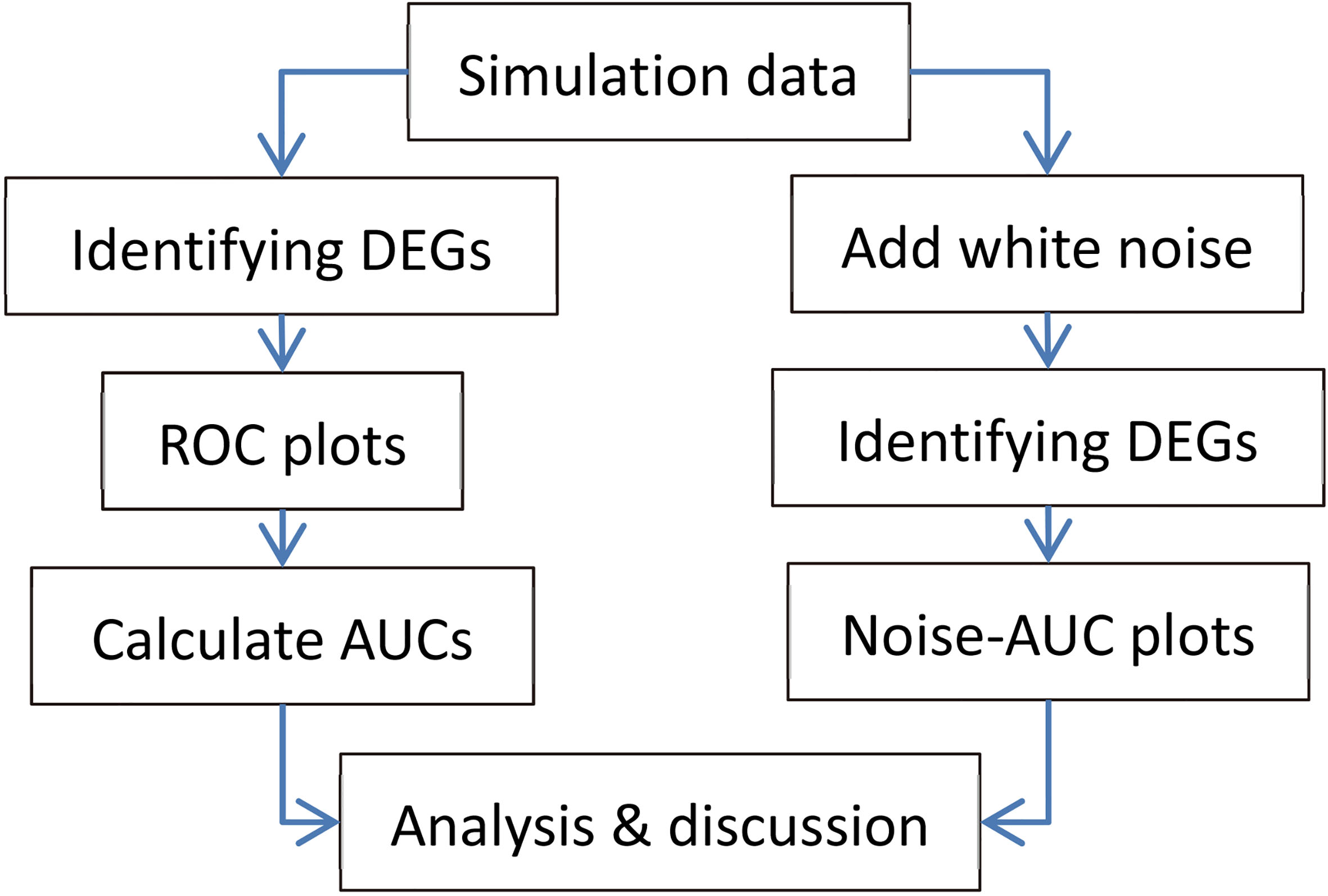
Figure 1 shows the flowchart of this study.

3.1Test the performance of identifying DEGs by MIC

Here, we used AUC to represent the performances of identifying DEGs of the methods. Let MIC and the four benchmarks mine the 2900 simulation datasets to identify DEGs, and calculate AUCs according to the identifying results of each method, and plot boxplots shown in Figs 2–5.

Figure 2.

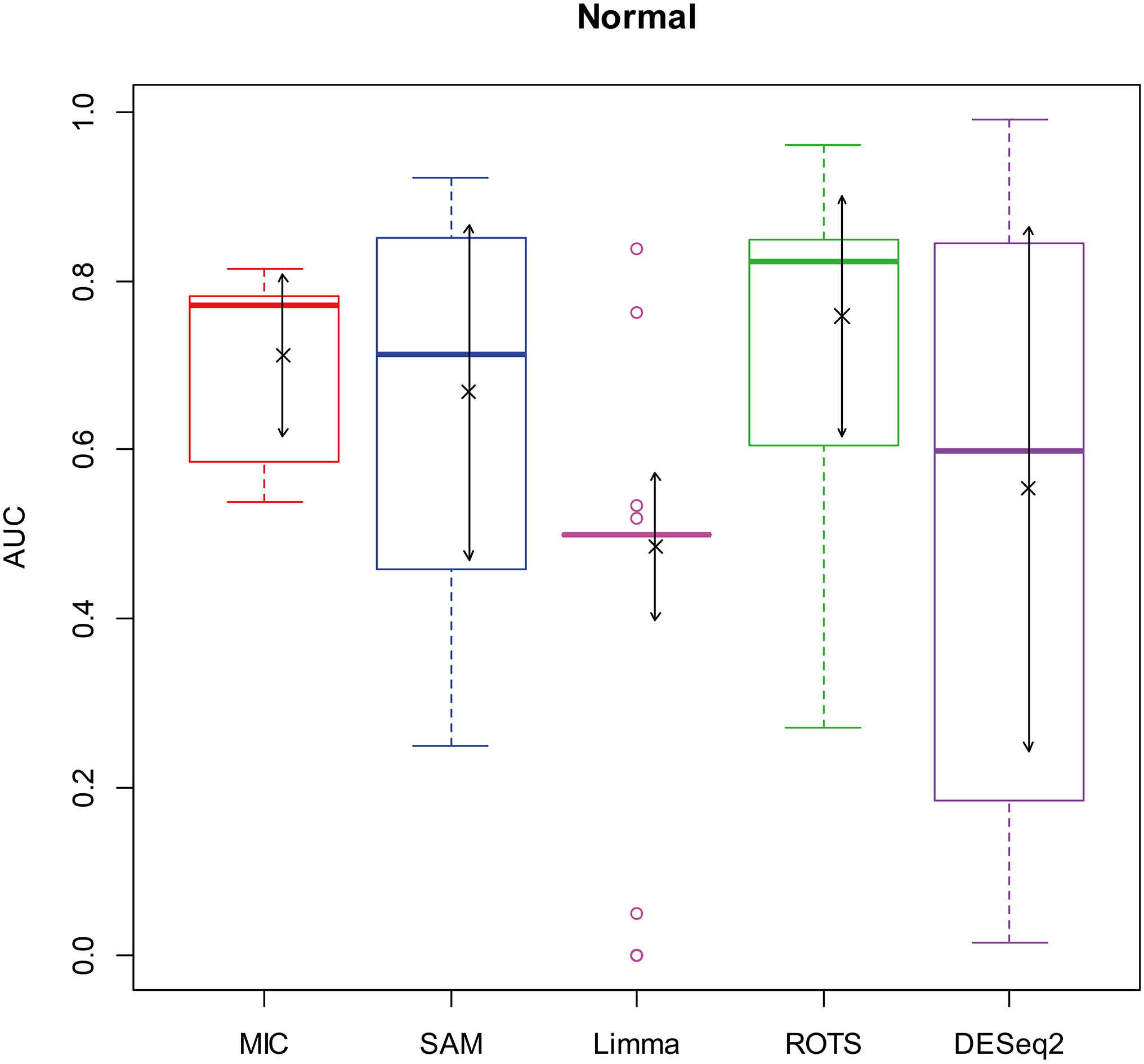
AUC boxplot on normal data. “×”s are the means. Bidirectional arrows represent ± 1 σ.

Figure 3.

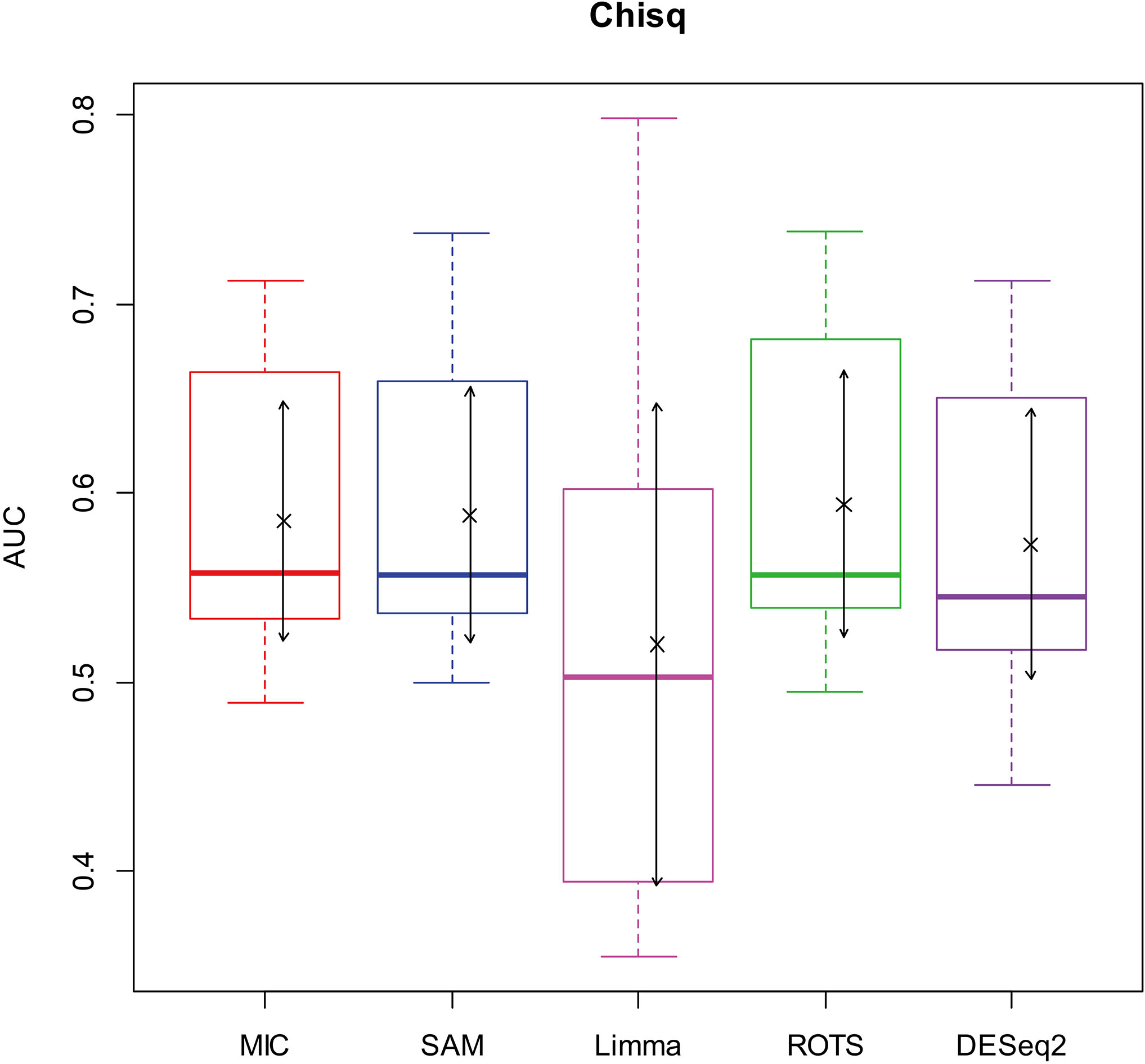
AUC boxplot on chi-square data. “×”s are the means. Bidirectional arrows represent ± 1 σ.

Table 2

The counts of AUC ⩽ 0.5

Method	AUC ⩽ 0.5	AUC < 0.5
MIC	5	5
SAM	301	301
Limma	1896	728
ROTS	35	35
DESeq2	535	535

Note: The counts are from the 2900 simulation datasets, one for each.

Figure 4.

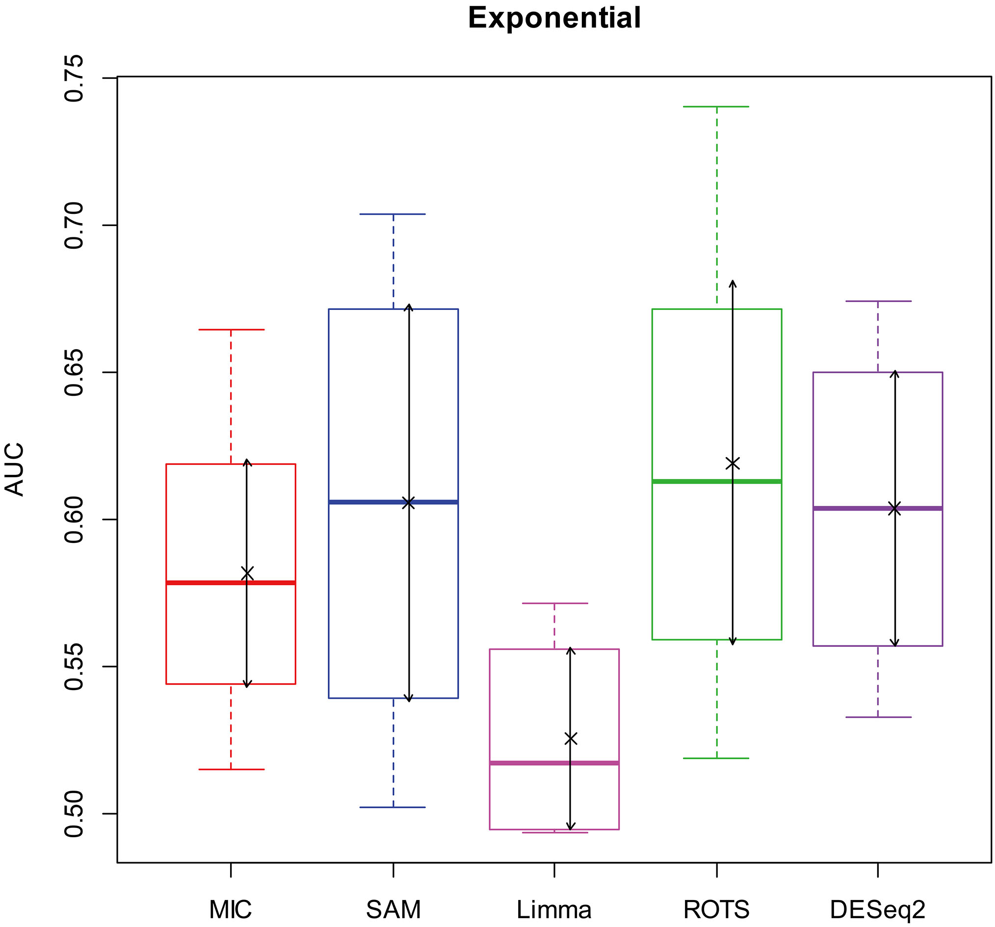
AUC boxplot on exponential data. “×”s are the means. Bidirectional arrows represent ± 1 σ.

Figure 5.

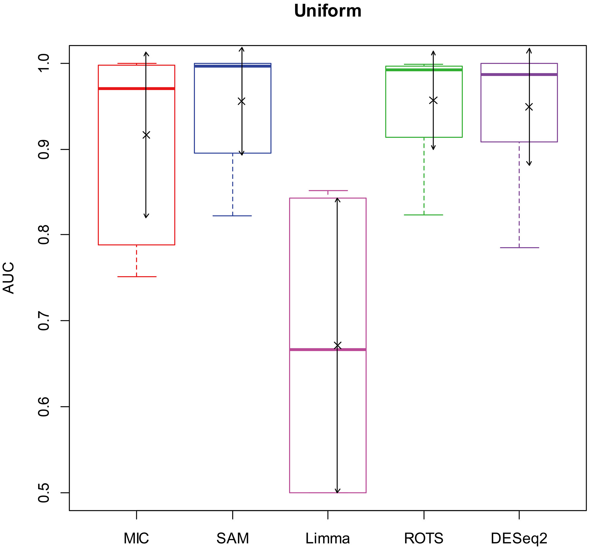
AUC boxplot on uniform data. “×”s are the means. Bidirectional arrows represent ± 1 σ.

In addition, since a method will lose its value to identify DEGs as AUC = 0.5, we also counted the case of AUC ⩽ 0.5 of the five methods (Table 2). In Table 2, both 5 of MIC are from the chi-squared datasets.

3.2Test the noise immunity of identifying DEGs by MIC

A real gene expression profile contains a large amount of noise [40]. It is an important index that the ability of a method to resist noise interference over identifying DEGs. To evaluate the noise immunity of a method, we simulate noise-bearing gene expression data by adding white noise on the simulated data.

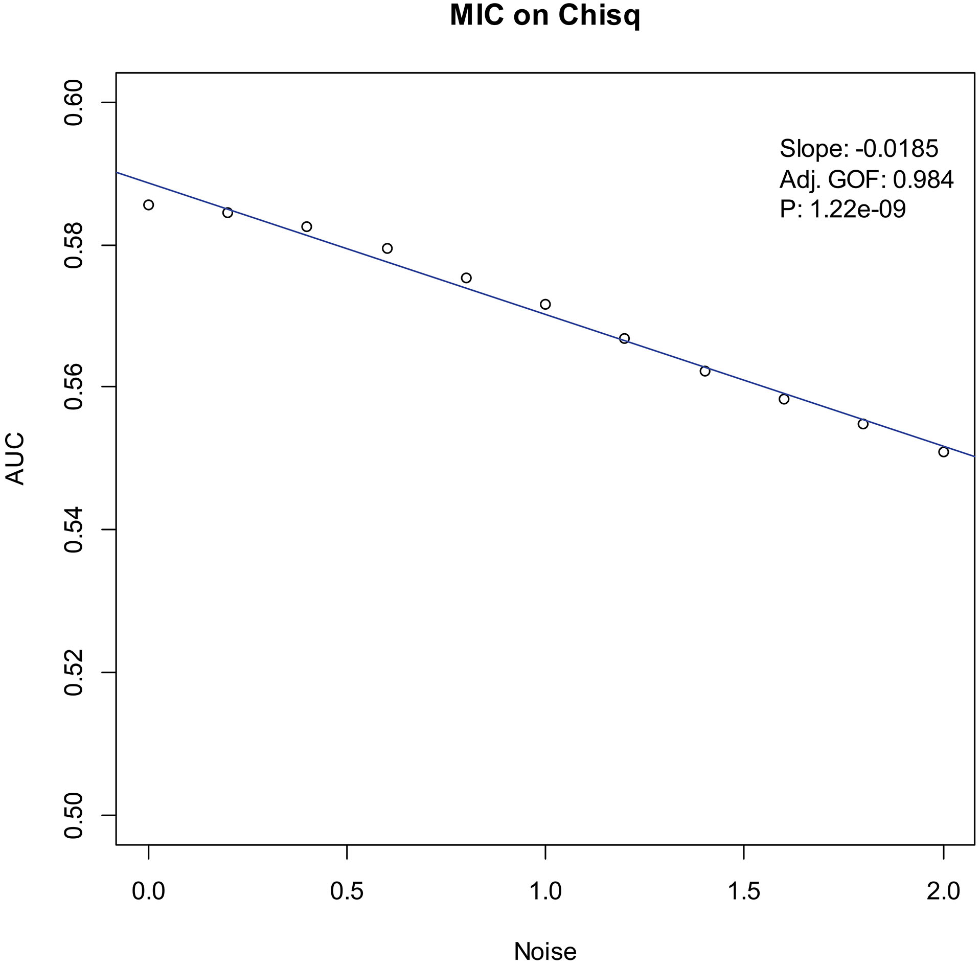
Our experiments show that the AUCs of all the methods in all the datasets are around 0.5 when the variance of white noise reaches to 2.0. Therefore, in the noise immunity experiments, we set the range to [0, 2.0] of the white noise added to the simulation datasets, with step of 0.2, a total of 11 levels of noise. For each noise level, all the methods identify DEGs and calculate the average AUCs grouped by the distributions. Then plot the scatter plots of Noise-AUC, and make linear fits to all points. Figures 6–9 show the plots of MIC and the Table 3 lists the summarization of all methods on the four distributions.

Table 3

The linear fits of Noise-AUC plots

Distribution	Method	Slope	Adj. GOF	P
Normal	MIC	-0.0920	0.914	2.71 × 10-6
	SAM	-0.0768	0.967	3.32 × 10-8
	DESeq2	-0.0157	0.482	1.06 × 10-2
	ROTS	-0.113	0.924	1.51 × 10-6
	Limma	0.00574	0.302	4.64 × 10-2
Chi-square	MIC	-0.0185	0.994	1.22 × 10-9
	SAM	-0.0142	0.957	1.17 × 10-7
	DESeq2	-0.00771	0.764	2.67 × 10-4
	ROTS	-0.0148	0.965	4.41 × 10-8
	Limma	0.00274	0.912	2.91 × 10-6
Exponential	MIC	-0.0294	0.988	4.17 × 10-10
	SAM	-0.035	0.991	1.27 × 10-10
	DESeq2	-0.0364	0.978	5.76 × 10-9
	ROTS	-0.0463	0.989	2.91 × 10-10
	Limma	-0.00447	0.179	0.108
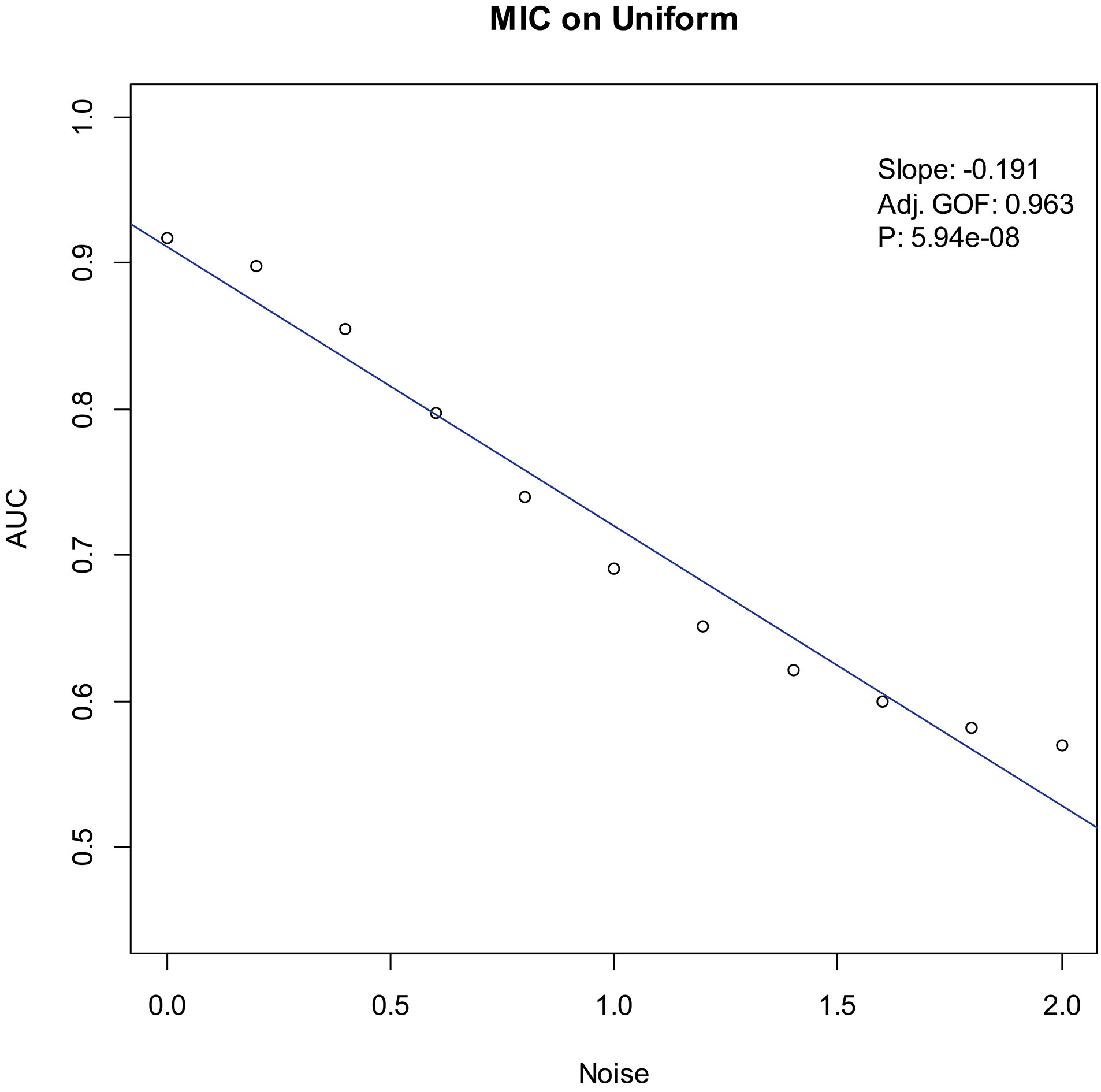
Uniform	MIC	-0.191	0.963	5.94 × 10-8
	SAM	-0.207	0.978	5.66 × 10-9
	DESeq2	-0.205	0.970	2.29 × 10-8
	ROTS	-0.203	0.976	9.12 × 10-9
	Limma	-0.0967	0.875	1.47 × 10-5

Note: “Slope” indicates the slope of the line, “Adj. GOF” is the adjusted goodness of fit, and “P” is the P-value of the fit.

Figure 6.

Noise-AUC plot of MIC on normal. The line is fitted by the points. “Slope” indicates the slope of the line, “Adj. GOF” is the adjusted goodness of fit, and “P” is the P-value of the fit.

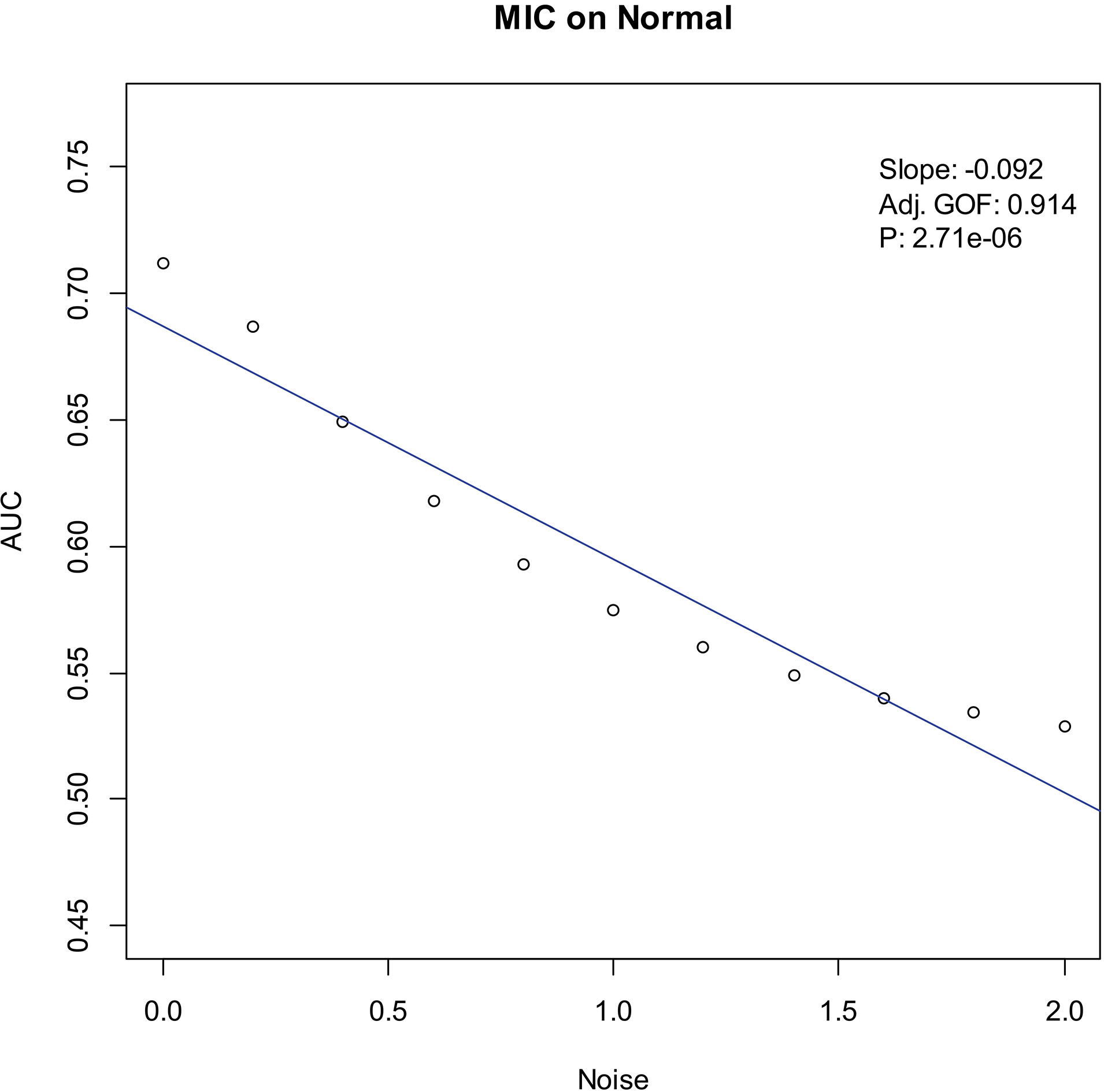
Figure 7.

Noise-AUC plot of MIC on chi-square. The line is fitted by the points. “Slope” indicates the slope of the line, “Adj. GOF” is the adjusted goodness of fit, and “P” is the P-value of the fit.

Moreover, we also recorded the curve fitting of each dataset, and counted the fitted line slopes greater than 0 for each method (Table 4).

Table 4

The counts of slope > 0

Method	Slope > 0
MIC	0
SAM	3
Limma	11
ROTS	0
DESeq2	8

Note: The counts are from the 29 groups of simulation datasets.

Figure 8.

Noise-AUC plot of MIC on exponential. The line is fitted by the points. “Slope” indicates the slope of the line, “Adj. GOF” is the adjusted goodness of fit, and “P” is the P-value of the fit.

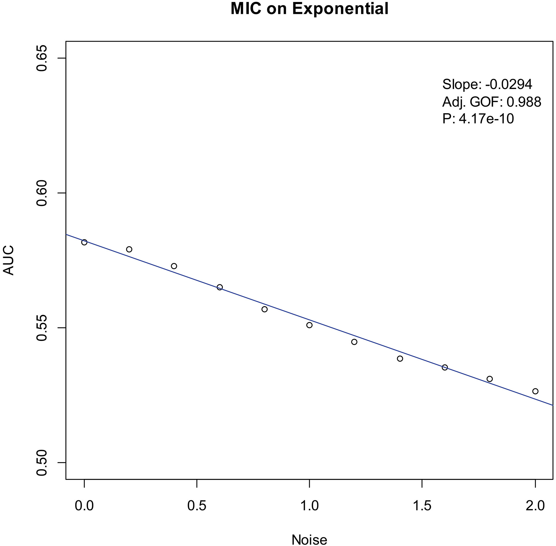
Figure 9.

Noise-AUC plot of MIC on uniform. The line is fitted by the points. “Slope” indicates the slope of the line, “Adj. GOF” is the adjusted goodness of fit, and “P” is the P-value of the fit.

4.Discussions

Differentially expressed gene identification is an application of data mining. It identifies genes with differential expression levels (variables) based on sample phenotypes (covariates). Therefore, the relationship between sample phenotype and expression level can be simplified into a model Eq. (3). Based on this model, differentially expressed genes can be screened by simply calculating the MIC values of all genes. The entire calculation process does not involve assumptions and calculations of any parameters.

4.1Performance of identifying DEGs by MIC

Figures 2–5 show that the AUCs of MIC are significantly better than the Limma’s (the AUCs of Limma are also significantly lower than the other benchmarks’). The AUC of MIC is ranked the first with SAM and ROTS in the chi-square distribution data, ranked second after ROTS (small 6.19%) in normal distribution, ranked 4th after SAM, ROTS and DESeq2 (small 3.94%, 6.07%, 3.66%, respectively) in exponential distribution, and also ranked 4th after the three methods (small 4.09%, 4.19%, 3.41%, respectively) in uniform distribution. If we only consider the ranks and difference percentage of AUCs, we can think that the performance of identifying DEGs by MIC is significantly better than Limma’s, which is almost same as the performances of SAM, ROTS and DESeq2. However, after further checking Figs 2–5, we can find that the feature of AUC variance of MIC is the best except for the uniform distribution, which is only 8.89% larger than Limma’s in the normal distribution. A smaller AUC variance means that the method is more adaptive to the data/environment, and less likely to be miscalculation affecting by the change of gene expression. Although the AUC variance MIC performs similarly to SAM, ROTS, and DESeq2 in uniform distribution, the density of gene expression is usually not uniform in reality.

In addition, it means a method has no value in practice when AUC = 0.5, and indicates a method has serious defects when AUC < 0.5. Based on analysing various types of data, the fewer AUC ⩽ 0.5 indicates that the method is more robust and adaptable to data/environment. Table 2 shows the counts of AUC ⩽ 0.5 in 2900 AUCs for each method. It indicates that the counts of MIC are greatly less than the other methods. Although Table 2 suggests that MIC has 5 AUCs less than or equal to 0.5 in the chi-square distribution datasets, it is only 0.417% of the 1200 chi-square datasets, accounting for 0.172% of all datasets.

In summary, compared with the existing methods, MIC method is in the first tier in the performance of identifying DEGs, and it has stronger robustness and higher data/environment adaptability.

4.2Noise immunity of identifying DEGs by MIC

The noise involved in a gene profile is an important factor affecting the accuracy of a method to identifying DEGs, especially for low expressed genes. In order to investigate the noise immunity of MIC, we tested its performance of identifying DEGs in a noisy environment by adding white noise to a noise-free dataset. For a method with excellent noise immunity, its AUCs should decrease with the increase of noise, and the slower decreasing, the stronger the noise immunity. Our experiments (Figs 6–9) show that the AUCs of each method have a good linear relationship with the noise intensity (the magnitudes of variance of the white noise). Thus, we linearly fit the AUCs to use the slope of the fitted line as a quantitative indicator for the noise immunity of a method. Obviously, the slope of the fitted line should be less than or equal to 0, and the smaller the absolute value, the stronger the noise immunity. By Limma, the slopes of the fitted lines in the normal and chi-square distribution shown in Table 3 are greater than 0. Meanwhile, Table 4 also shows that the method has up to 11 groups with a slope greater than 0 (accounting for up to 37.9%, significantly higher than the other 4 methods). Moreover, Limma is also greatly weaker than the other four methods in performance of identifying DEGs. Therefore, we consider to remove Limma from the next step in the noise immunity test.

In the noise immunity test shown Figs 6–9 and Table 3, the slope of fitted line of MIC is nearly same as SAM and ROTS in the normal data, whose absolute value is larger than DESeq2. And, the slope is almost same as SAM, ROTS and DESeq2 among the other three distributions. Furthermore, in the counts of the fitted line slope shown in Table 4, MIC and ROTS have no slope is greater than 0, while SAM and DESeq2 have 3 and 8, respectively.

In summary, compared with the existing methods, MIC is also in the first tier in terms of noise immunity.

4.3Advantages and disadvantages of MIC

MIC is a non-parametric statistic with good noise immunity. It has better ability to discover non-function relations than the ordinary methods in exploring two-variable relationships. And, it has better uniformity to functional relationships [28] (i.e., MIC can yield almost the same value regardless of the functional relationship). In general, a gene expression data contains amount of noise [40], and the functional relationship between phenotype and expressed values is not clear, making MIC very suitable for the analysis of gene expression.

The deficiencies of MIC are mainly reflected in the fact that it is an exhaustive algorithm, leading its runtime is not more advantageous than the methods including permutation such as SAM, ROTS and DESeq2. When we use MIC to process very large datasets, its algorithmic time is a factor that must be considered. In addition, the essence of MIC is to replace all points in the dataset with some grids on a two-dimensional plane. Since the number of grids is not infinite, it is only an approximate method, being reduced accuracy of the algorithm. And thirdly, compared with the existing methods, although MIC performance is in the first tier, our experiments show that it has a few results of AUC < 0.5, indicating that it may yield false positives. It needs to be optimized in further studies.

Our experiments verify that MIC is feasible to identify differentially expressed genes, and its performance of identifying DEGs and noise immunity are in the first tier of the existing methods, and it has advantage with more robustness and adaptability. Since the distributions of gene expression may be diverse, our experiments did not involve more distributions. And, we did not test the runtime of the algorithm. These might be further studied in the future.

Acknowledgments

This research was supported by the National Natural Science Foundation of China (Grant no. 31660321).

Conflict of interest

None to report.

References

[1]	Velculescu VE, et al., Serial Analysis of Gene Expression. Science, (1995) ; 270: (5235): 484-487.
[2]	Brown PO, Botstein D. Exploring the new world of the genome with DNA microarrays. Nature Genetics, (1999) ; 21: : 33-37.
[3]	Xiang CC, Chen Y. cDNA microarray technology and its applications. Biotechnology Advances, (2000) ; 18: (1): 35-46.
[4]	Heller G, Zielinski CC, Zochbauermuller S. Lung cancer: From single-gene methylation to methylome profiling. Cancer and Metastasis Reviews, (2010) ; 29: (1): 95-107.
[5]	Derisi JL, et al., Use of a cDNA microarray to analyse gene expression patterns in human cancer. Nature Genetics, (1996) ; 14: (4): 457-460.
[6]	Ideker T, et al., Testing for differentially-expressed genes by maximum-likelihood analysis of microarray data. Journal of Computational Biology, (2000) ; 7: (6): 805-817.
[7]	Robinson MD, Mccarthy DJ, Smyth GK. edgeR: a Bioconductor package for differential expression analysis of digital gene expression data. Bioinformatics, (2010) ; 26: (1): 139-140.
[8]	Schena M, et al., Quantitative Monitoring of Gene Expression Patterns with a Complementary DNA Microarray. Science, (1995) ; 270: (5235): 467-470.
[9]	Newton MA, et al., On differential variability of expression ratios: improving statistical inference about gene expression changes from microarray data. Journal of Computational Biology, (2001) ; 8: (1): 37-52.
[10]	Lonnstedt I. Replicated microarray data. Statistica Sinica, (2001) ; 12: (1): 31-46.
[11]	Smyth GK, Linear models and empirical bayes methods for assessing differential expression in microarray experiments. Statistical Applications in Genetics and Molecular Biology, (2004) ; 3: (1): 1-28.
[12]	Dudoit S, et al., Statistical methods for identifying differentially expressed genes in replicated cdna microarray experiments. Statistica Sinica, (2002) ; 12: (1).
[13]	Zhao Y, Pan W. Modified nonparametric approaches to detecting differentially expressed genes in replicated microarray experiments. Bioinformatics, (2003) ; 19: (9): 1046-1054.
[14]	Tusher VG, Tibshirani R, Chu G. Significance analysis of microarrays applied to the ionizing radiation response. Proceedings of the National Academy of Sciences of the United States of America, (2001) ; 98: (9): 5116-5121.
[15]	Elo LL, et al., Reproducibility-optimized test statistic for ranking genes in microarray studies. IEEE/ACM Transactions on Computational Biology and Bioinformatics, (2008) ; 5: (3): 423-431.
[16]	Baldi P, Long AD. A Bayesian framework for the analysis of microarray expression data: Regularized t-test and statistical inferences of gene changes. Bioinformatics, (2001) ; 17: (6): 509-519.
[17]	Breitling R, et al., Rank products: a simple, yet powerful, new method to detect differentially regulated genes in replicated microarray experiments. FEBS Letters, (2004) ; 573: (1): 83-92.
[18]	Broberg P, Ranking genes with respect to differential expression. Genome Biology, (2002) ; 3: (9): 1-23.
[19]	Efron B, et al., Empirical Bayes Analysis of a Microarray Experiment. Journal of the American Statistical Association, (2001) ; 96: (456): 1151-1160.
[20]	Smyth GK. limma: Linear models for microarray data. Bioinformatics & Computational Biology Solutions Using R & Bioconductor, (2005) ; 397-420.
[21]	Seyednasrollah F, et al., ROTS: reproducible RNA-seq biomarker detector – prognostic markers for clear cell renal cell cancer. Nucleic Acids Research, (2016) ; 44: (1): 1.
[22]	Pursiheimo A, et al., Optimization of statistical methods impact on quantitative proteomics data. Journal of Proteome Research, (2015) ; 14: (10): 4118-4126.
[23]	Albrecht U, Bowman KD. Gene expression in Citrus sinensis (L.) Osbeck following infection with the bacterial pathogen candidatus liberibacter asiaticus causing huanglongbing in florida. Plant Science, (2008) ; 175: (3): 291-306.
[24]	Kim J, et al., Response of Sweet orange (citrus sinensis) to ’candidatus liberibacter asiaticus’ infection: microscopy and microarray analyses. Phytopathology, (2009) ; 99: (1): 50-57.
[25]	Anders S, Huber W. Differential expression analysis for sequence count data. Genome Biology, (2010) ; 11: (10): 1-12.
[26]	Love MI, Huber W, Anders S. Moderated estimation of fold change and dispersion for RNA-seq data with DESeq2. Genome Biology, (2014) ; 15: (12): 550-550.
[27]	Jain N, et al., Local-pooled-error test for identifying differentially expressed genes with a small number of replicated microarrays. Bioinformatics, (2003) ; 19: (15): 1945-1951.
[28]	Reshef DN, et al., Detecting novel associations in large data sets. Science, (2011) ; 33: (6062): 1518-1524.
[29]	Liu H, et al., A novel method for identifying SNP disease association based on maximal information coefficient. Genetics and Molecular Research, (2014) ; 13: (4): 10863-10877.
[30]	Liu H, et al., Modified bagging of maximal information coefficient for genome-wide identification. Int. J. Data Mining and Bioinformatics, (2016) ; 14: (3): 229-257.
[31]	Han-Ming L, et al., Maximal information coefficient on identifying differentially expressed genes of permanent atrial fibrillation. Chinese Journal of Biomedical Engineering, (2015) ; 3: (1): 8-16.
[32]	Hanming L, Dan Y. The application of maximum information coefficient in the identification of miRNA expression differences in valvular heart disease. China Sciencepaper, (2017) ; 12: (6): 707-711.
[33]	Wenfeng Q, Hanming L. Identifying differentially expressed genesof citrus huanglongbing disease based on maximal information coefficient. Journal of Gannan Normal University, (2018) (3).
[34]	Kim SY, Lee JW, Sohn IS. Comparison of various statistical methods for identifying differential gene expression in replicated microarray data. Statistical Methods in Medical Research, (2006) ; 15: (1): 3-20.
[35]	Wen-Juan S, Chun-Fa T, Ji-Sen S. Comparison of statistical methods for detecting differential expression in microarray data. Hereditas, (2008) ; 30: (12): 1640-1646.
[36]	Student, The probable error of a mean. Biometrika, 1908; 6(1): 33-57.
[37]	Gentleman RC, et al., Bioconductor: open software development for computational biology and bioinformatics. Genome Biology, (2004) ; 5: (10): 1-16.
[38]	Albanese D, et al., minerva and minepy: a C engine for the MINE suite and its R, Python and MATLAB wrappers. Bioinformatics, (2013) ; 29: (3): 407-408.
[39]	Racine JS. RStudio: A Platform-Independent IDE for R and Sweave. Journal of Applied Econometrics, (2012) ; 27: (1): 167-172.
[40]	Raser JM, Oshea EK. Noise in gene expression: origins, consequences, and control. Science, (2005) ; 309: (5743): 2010-2013.