Effect of ventricular myocardium characteristics on the defibrillation threshold

1.Background and objective

In China, more than 500,000 people die each year from sudden cardiac death (SCD) [1]; worldwide, this figure has reached an alarming 7 million [2]. One of the important causes of SCD is ventricular fibrillation, and the only effective clinical way to terminate it is by shock defibrillation. Myocardial characteristics play an important role in shock defibrillation effect, which differs markedly under different pathological or physiological conditions of different individuals. For instance, cardiomyocyte coupling will decrease with age; myocardial ischemia can lead to cardiomyocyte decoupling at the ischemic area; the degree of myocardial anisotropy increases for the patients with cardiac hypertrophy. Therefore, it is instructive to understand the effect of ventricular myocardium characteristics on the defibrillation threshold (DFT). A wrong assessment of DFT will result in a failed shock defibrillation [3]. Therefore, studying the effect of myocardium characteristics on defibrillation has not only important theoretical significance, but also important clinical value.

The distribution of electric field in the heart is closely related to the defibrillation results [4]. It is almost impossible to measure the distribution of electric field in the myocardium in vivo, so finite-element (FE) modeling has been widely used in such studies. During the previous three decades, various three-dimensional cardiac models have been established. Among them, volume conductor models can best reflect the electric field distribution in ventricles. Some examples include the human thoracic model constructed by Camacho et al. [5], the dog chest model developed by Karlon et al. [6], and the human thoracic model built by Kinst et al. [7]. Besides electric field, these models used current density as an indicator of defibrillation effects, which aimed to finding the relationship between current density and DFT. In 1975, the embryonic form of the critical mass hypothesis was proposed [8] and in the mid-nineties, this method for calculating the DFT has been generally accepted [9]. Using this hypothesis, many models were established to study the effect of defibrillation field on DFT, such as the porcine thoracic model constructed by Wang et al. [10] and the dog heart model built by Yang et al. [11]. With the understanding of the influence of myocardial anisotropy on the distribution of defibrillation electric field [12, 13], several cardiac volume conductor models have reported factors influencing the myocardial fibers. Such as the human torso models constructed by Eason et al. [13], Aguel et al. [14], Wang et al. [15] and Modre et al. [16], and the swine chest models constructed by Panescu et al. [17].

The aforementioned studies were committed to optimizing the electrode configuration [5, 6, 7, 10, 11] or researching the effects of myocardial anisotropy on DFT based on one group of anisotropic conductivities, which did not further discuss why fiber anisotropy could have this kind of effect on DFT [13, 14, 15, 16, 17].

To investigate the effect of myocardial characteristics on DFT, this manuscript used a rabbit ventricle as the anatomical model, which has higher resolution than aforementioned models [5, 6, 7, 10, 11, 14, 15, 16, 17, 18]. Rabbit heart has much smaller size compared to human heart, so using this model can evidently reduce the computational complexity, significantly shortening the simulation time. In addition, the structure and electrophysiological characteristics of the human and rabbit heart have a high degree of similarity, making this model reliable [19].

In this manuscript, the DFTs in different ventricular myocardium characteristics were given in the RESULTS section. The effects of cardiomyocyte coupling, the degree of myocardial anisotropy and the combined effects of these two factors on DFT were discussed in DISCUSSION section. Model development, model parameter selection and simulation methods were discussed in METHODS section. This study provided a basis for the modeling and parameter selection of myocardial conductivity in different conditions, and thus provides some guidance for defibrillation treatment.

2.Methods

In this manuscript, a rabbit ventricular FE model with a resolution of approximately 250 μm was constructed using the magnetic resonance imaging (MRI) data of the rabbit ventricles provided by Oxford University [20, 21]. The model is 2.37 × 2.16 × 2.94 cm and contains 955,292 nodes and 50,28,264 elements. In this model, conductivity value was used to represent the cardiomyocyte coupling, and the ratio of anisotropic conductivity was used to represent the degree of myocardial anisotropy. By changing the value of the anisotropic conductivity, we studied the effect of myocardium characteristics on the DFTs based on the critical mass hypothesis. The criterion used in this study was a voltage gradient of 5 V/cm generated over 95% of the myocardium [22].

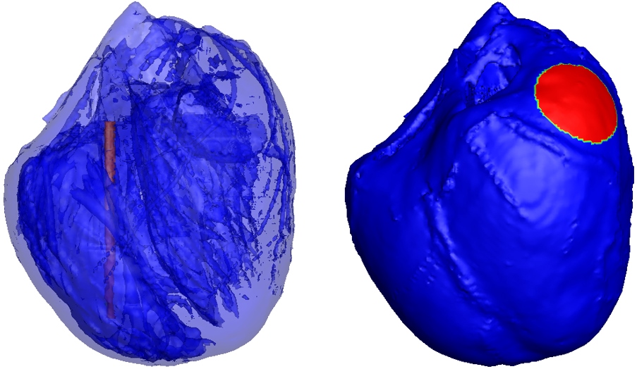
To simplify the problem, all simulations in this manuscript used the implantable cardioverter defibrillator (ICD) electrode configuration: the anode (a thin cylindrical electrode with a height of 16 mm and a radius of 0.5 mm) was inserted into the right ventricular cavity and the cathode (a circular patch electrode with 4 mm radius) was placed on the upper part of the left ventricular epicardium (Fig. 1). A defibrillation threshold voltage was applied between the cylindrical electrode (anode) and the circular patch electrode (cathode) such that the critical mass hypothesis was met. In this study, the DFTs for isotropic, anisotropic, and different anisotropic conductivities were simulated.

Figure 1.

ICD electrode configuration was used in the simulation. The red part of in the right ventricle as shown in left picture is the columnar electrode, the red part of on left ventricular epicardium as shown in right picture is the circular patch electrodes.

The electric shock defibrillation problem is equivalent to the constant electric field problem in the volume conductor model. The potential in the volume conductor satisfies the Laplace equation:

where σ is the conductivity tensor, and Φ is the potential. Equation (1) is solved subject to the Dirichlet condition Eq. (2) for the anode and cathode regions, and the Neumann boundary condition for the residual ventricular surface Eq. (3).

Equation (2) represents the Dirichlet boundary condition, which defines the myocardial surface (S⁢Ii) in contact with the electrode (ith) with a potential Vi, and the potential of S⁢Ii is Vi. Equation (3) represents the Neumann boundary condition, which defines the myocardial surface that is not in contact with the electrode; the derivative of the potential gradient on the surface of the myocardium is zero. The finite element method can be used to solve Eq. (1) [5] because it is a numerical simulation technique suitable for solving partial differential equations in an irregular geometric region.

The fiber conductivity tensor σ of every element in FE model was calculated using following formula [21]:

where the coefficient σl is the conductivity along the direction of the myocardial fibers, and the coefficient σt is the conductivity perpendicular to the myocardial fiber. I is the unit matrix. A, the direction cosine of every element, can be obtained by the rule-based approach [23], which determines the direction of myocardial fibers. Therefore, this model reflects the fiber orientation in ventricular epicedial, myocardial, and endocardial layers.

The FE simulation software, Comsol Multiphysics 5.2 (COMSOL Inc.), was used. For an isotropic cardiac volume model, the electrical conductivity of myocardial fibers was set to σm= 0.25 S/m (first row, Table 1). Ventricular blood perfusion greatly changes the distribution of the electric field in the volume conductor model, which has a great impact on the DFT, so the blood perfusion was added into the ventricle. Since blood conductivity is isotropic, for all ventricular models constructed in this study, the conductivity of the intraventricular blood was set to σb= 0.7 S/m (the average of the blood conductivities in Table 1).

Figure 2.

Simulation result of the distribution of ventricular electric field. The red part represents the high electric field area and the blue part represents the low electric field area. The unit of electrical field (EF) is V/cm.

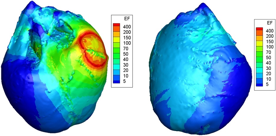
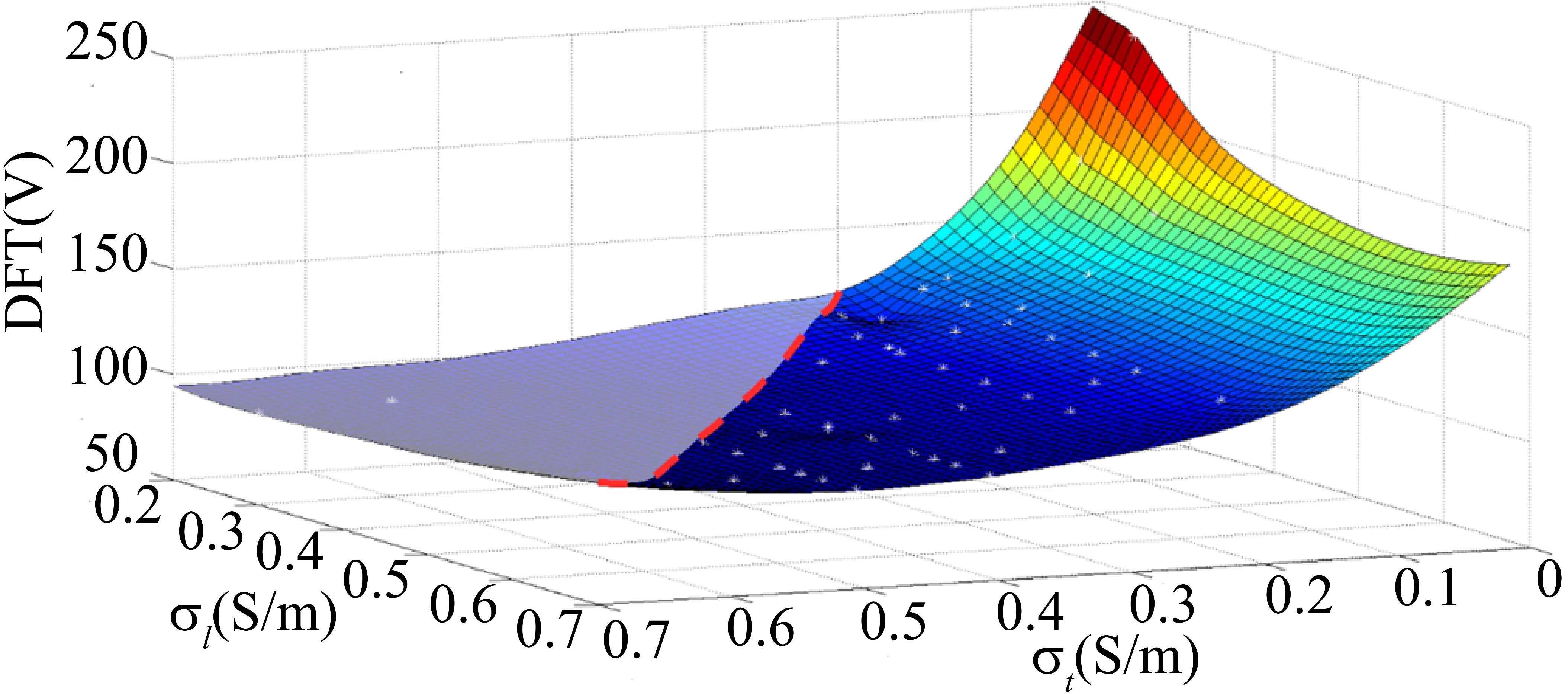
Figure 3.

Effect of cell coupling degree on defibrillation electric field distribution. As shown, the two axes of the horizontal plane respectively represent electrical conductivity along the myocardial fiber σl and perpendicular to the myocardial fiber σt, and the axis perpendicular to the horizontal plane represents the DFT. The white dots distributed over the curved surface represent the simulated DFT. As the myocardial fiber conductivity reflects the cell coupling, follow the two restrictions mentioned above, the right side of the red dotted line is the actual possible DFTs distribution.

3.Results

Electrical conductivity of myocardial fibers varies in different literatures. For all myocardial conductivities shown in Table 1, the corresponding distributions of electric field in the ventricle were gotten by our computer simulation (Fig. 2). The DFT (minimum defibrillation voltage that meets the critical mass hypothesis) is showed in seventh column of Table 1. Using Eq. (4), we calculated all the percentages of difference (POD, eighth column, Table 1) between the DFT of isotropic conductivity (DFTIso) and the DFT of anisotropic conductivity (DFTAni).

The values of anisotropic conductivites were changed depending on the possible cell coupling conditions: 1. because the cells are not prone to over-coupling, the σl and σt values were < 0.7 S/m (all myocardial conductivities given in literature [5, 13, 14, 15, 16, 17] are below 0.7 S/m); 2. usually the number of gap junctions along the cell fibers is more than those perpendicular to the cell fibers; therefore, σl⩾σt. Based on these two principles, the DFTs were obtained by simulation, resulting in a curved surface (Fig. 3). The effect of the anisotropy on the DFT is further explained in Fig. 4, which showed the percentage of ventricular myocardial mass below discrete potential gradients in different myocardial coupling (conductivity).

In the next part, three aspects of the problem will be discussed: 1. The effect of intercellular coupling on the DFT, which was represented as the value of the conductivity in volume conductor model (Section 3.1); 2. The effect of the degree of the myocardial anisotropy on the DFT, which was represented as the ratio of anisotropic conductivity in volume conductor model (Section 3.2); 3. The combined effect of the above two aspects on the DFT (Section 3.3).

3.1Effects of intercellular coupling of cardiomyocytes on the defibrillation thresholds

Studies have shown that cardiomyocyte coupling directly affects the degree of dispersion in myocardial repolarization and provides a major basis for reentrant arrhythmias [24]. This section investigated the effects of the degree of cardiomyocyte coupling on the DFT. By comparing the DFTs when σ¯= 0.2526 S/m (second row, Table 1) and σ¯= 0.375 S/m (sixth row, Table 1), whose ratios of anisotropic conductivity are both 2:1, it was found that the DFTs are 122 V and 107 V respectively. Therefore, the tighter the intercellular coupling is, the greater the myocardium conductivity which results in the lower DFT. This is because when the electrical conductivity of the myocardium is lower, more current flows through the blood, reducing the electric field strength in the myocardium. As a result, to satisfy the critical mass hypothesis, a higher defibrillation voltage must be applied for successful defibrillation.

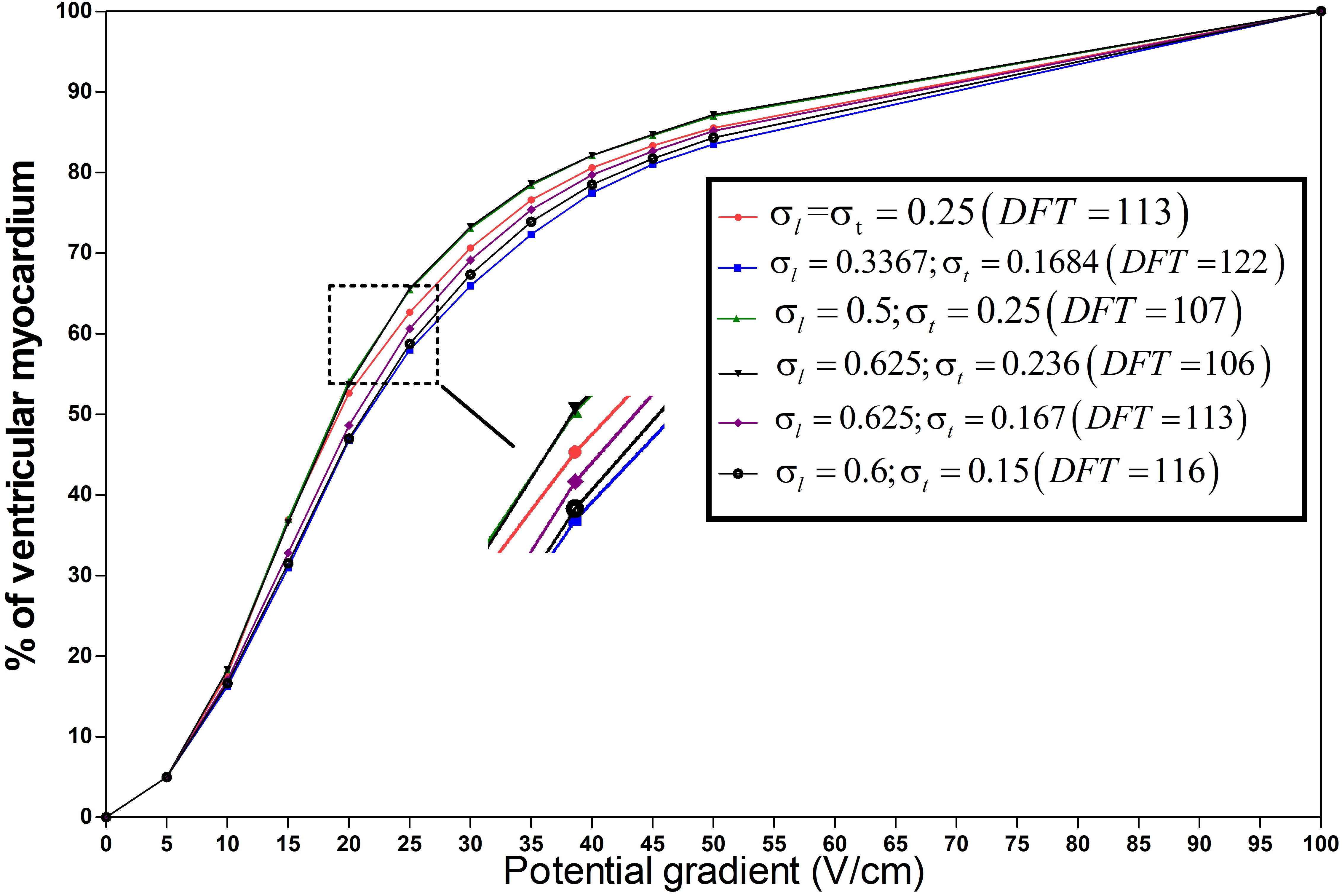
Figure 4.

The percentage of ventricular myocardial mass below discrete potential gradients in different anisotropic conductivity. The right diagram shows the case in Table 1 with different anisotropy ratios(σl/σt), which are 1:1, 2:1, 2:1, 2.648:1, 3.74:1, 4:1 respectively. The units of conductivity σl and σt are S/m, the units of DFTs are V.

4.Conclusions

This study focused on the effects of ventricular myocardium characteristics on DFT. It is concluded that the DFTs and electrical conductivity of myocardial fibers are closely related. Higher electrical conductivities correlates with lower DFTs. In addition, the DFTs are affected by the degree of myocardial anisotropy. Higher degree of myocardial anisotropy correlates with higher DFTs.

Cardiac modeling and simulation are important techniques for evaluating defibrillation electric field distribution; the accuracy and complexity of the model directly affect the simulation results and efficiency. This study not only provides a basis for cardiac modeling and simulation of defibrillation electric field distribution, but also provides a new insight into the differences in the DFTs of clinical patients.

References

[1] | Hua W, Zhang L, Wu Y, et al. Incidence of sudden cardiac death in china analysis of 4 regional populations. Journal of the American College of Cardiology (2009) ; 54: (12): 1110-1118. |
[2] | Smith TW, Cain ME. Sudden cardiac death: Epidemiologic and financial worldwide perspective. Journal of Interventional Cardiac Electrophysiology (2007) ; 17: (3): 199-203. |
[3] | Li Y, Ristagno G, Yu T, et al. A comparison of defibrillation efficacy between different impedance compensation techniques in high impedance porcine model. Resuscitation (2009) ; 80: (11): 1312-1317. |
[4] | Jianfei W, Lian J, Xiaomei W, et al. Low-energy defibrillation research using a rabbit ventricular model: Optimizing the potential gradient distribution using multiple epicardial electrodes. Conference Proceedings Annual International Conference of the IEEE Engineering in Medicine and Biology Society. IEEE Engineering in Medicine and Biology Society. Annual Conference (2016) ; 2753-2756. |
[5] | Camacho MA, Lehr JL, Eisenberg SR. A 3-dimensional finite-element model of human transthoracic defibrillation-paddle placement and size. IEEE Transactions on Biomedical Engineering (1995) ; 42: (6): 572-578. |
[6] | Karlon WJ, Eisenberg SR, Lehr JL. Effects of paddle placement and size on defibrillation current distribution – a 3-dimensional finite-element model. IEEE Transactions on Biomedical Engineering (1993) ; 40: (3): 246-255. |
[7] | Kinst TF, Sweeney MO, Lehr JL, et al. Simulated internal defibrillation in humans using an anatomically realistic three-dimensional finite element model of the thorax. Journal of Cardiovascular Electrophysiology (1997) ; 8: (5): 537-547. |
[8] | Zipes DP, Fischer J, King RM, et al. Termination of ventricular-fibrillation in dogs by depolarizing a critical amount of myocardium. American Journal of Cardiology (1975) ; 36: (1): 37-44. |
[9] | Aguel F, Eason JC, Trayanova NA, et al. Impact of transvenous lead position on active-can ICD defibrillation: A computer simulation study. Pace-Pacing and Clinical Electrophysiology (1999) ; 22: (12): 158-164. |
[10] | Wang YQ, Schimpf PH, Haynor DR, et al. Analysis of defibrillation efficacy from myocardial voltage gradients with finite element modeling. IEEE Transactions on Biomedical Engineering (1999) ; 46: (9): 1025-1036. |
[11] | Yang F, Sha Q, Patterson RP. A novel electrode placement strategy for low-energy internal cardioversion of atrial fibrillation: A simulation study. International Journal of Cardiology (2012) ; 158: (1): 149-152. |
[12] | Plonsey R, Barr R. The 4-electrode resistivity technique as applied to cardiac-muscle. IEEE Transactions on Biomedical Engineering (1982) ; 29: (7): 541-546. |
[13] | Eason J, Schmidt J, Dabasinskas A, et al. Influence of anisotropy on local and global measures of potential gradient in computer models of defibrillation. Annals of Biomedical Engineering (1998) ; 26: (5): 840-849. |
[14] | Aguel F, Eason JC, Trayanova NA, et al. Impact of transvenous lead position on active-can ICD defibrillation: A computer simulation study. Pace-Pacing and Clinical Electrophysiology (1999) ; 22: (12): 158-164. |
[15] | Wang YQ, Haynor DR, Kim Y. An investigation of the importance of myocardial anisotropy in finite-element modeling of the heart: Methodology and application to the estimation of defibrillation efficacy. IEEE Transactions on Biomedical Engineering (2001) ; 48: (12): 1377-1389. |
[16] | Modre R, Seger M, Fischer G, et al. Cardiac anisotropy: Is it negligible regarding noninvasive activation time imaging? IEEE Transactions on Biomedical Engineering (2006) ; 53: (4): 569-580. |
[17] | Panescu D, Webster JG, Tompkins WJ, et al. Optimization of cardiac defibrillation by 3-dimensional finite-element modeling of the human thorax. IEEE Transactions on Biomedical Engineering (1995) ; 42: (2): 185-192. |
[18] | Eason J, Schmidt J, Dabasinskas A, et al. Influence of anisotropy on local and global measures of potential gradient in computer models of defibrillation. Annals of Biomedical Engineering (1998) ; 26: (5): 840-849. |
[19] | Arevalo HJ, Boyle PM, Trayanova NA. Computational rabbit models to investigate the initiation, perpetuation, and termination of ventricular arrhythmia. Progress in Biophysics and Molecular Biology (2016) ; 121: (2): 185-194. |
[20] | Bordas R, Gillow K, Lou Q, et al. Rabbit-specific ventricular model of cardiac electrophysiological function including specialized conduction system. Progress in Biophysics and Molecular Biology (2011) ; 107: (1): 90-100. |
[21] | Clayton RH, Panfilov AV. A guide to modelling cardiac electrical activity in anatomically detailed ventricles. Progress in Biophysics and Molecular Biology (2008) ; 96: (1-3): 19-43. |
[22] | Jolley M, Stinstra J, Pieper S, et al. A computer modeling tool for comparing novel ICD electrode orientations in children and adults. Heart Rhythm (2008) ; 5: (4): 565-572. |
[23] | Bishop MJ, Plank G, Burton RAB, et al. Development of an anatomically detailed MRI-derived rabbit ventricular model and assessment of its impact on simulations of electrophysiological function. AJP: Heart and Circulatory Physiology (2010) ; 298: (2): H699-H718. |
[24] | Spach MS. Changes in the topology of gap-junctions as an adaptive structural response of the myocardium. Circulation (1994) ; 90: (2): 1103-1106. |